DOI: 10.13164/re.2016.0658 OPTICAL COMMUNICATIONS
Optimized FSO System Performance
over Atmospheric Turbulence Channels
with Pointing Error and Weather Conditions
Omar HASAN, Mohamed TAHA
Dept. of Communication Engineering, Princess Sumaya University for Technology, Amman, Jordan, 11941
[email protected], [email protected]
Manuscript received April 27, 2016
Abstract. In this paper, Bit Error rate and probability of outage are derived in closed form for plane wave mode over Gamma-Gamma free space optical channel under the influence of pointing errors and different weather condi-tions. The free-space optical system under study assumes deployment of intensity modulation / direct detection with on-off keying data formats. To evaluate the performance of the system using the derived expressions, two independent optimization algorithms were applied to find optimum system and channel parameters that optimize the perfor-mance of the two system metrics, i.e., bit error rate and probability of outage. The optimized system results were shown for different values of channel strength, weather conditions, optimum beamwidths and pointing error jitter variances. For each case, the optimized results are pro-vided as a function of the transmitted power or average received power.
Keywords
Bit Error Rate (BER), Free Space Optical Channel (FSO), Intensity Modulation (IM), Direct Detection (DD) with On-Off Keying (OOK), pointing error, jitter variance
1.
Introduction
Recent deployment of 4G technology resulted in great challenges to cellular carriers to increase backhaul capacity between cell towers. This increase in capacity is necessary to meet fast growing demands for mobile users acquiring deployment of 4G internet services. However, current installed microwave backhaul links cannot attain full 4G download speed for mobile users, hence, limiting number of users that can access the mobile network. On the other hand, optical cable technology can meet demands for higher speed data rates between backhaul cells, but its implementation can be difficult and expensive task due to different terrain types between backhaul cells. Free space optical (FSO) links can be a solution to meet growing de-mands by cellular carriers for higher link capacity as shown
by [1]. It was shown by [1], FSO systems using ultrashort pulse (USP) lasers developed by [2], can provide 1 Gbits/sec and 10 Gbits/sec backhaul capacity for 2 km – 3 km backhaul distances in all weather conditions. In addi-tion, FSO technology is low power, cost effective, no deployment licensing is required and can meet higher data rate capacity of future wireless technology such 5G.
However, transmission of optical signals through FSO channels can be degraded due to atmospheric turbulence, pointing error and weather attenuations. Weather condi-tions such as rain, snow, haze and fog can highly degrade the optical signal and limit its coverage. In dense foggy weather conditions, an optical signal with operating wave-length 1550 nm can experience an attenuation of 270 dB per km [3] limiting link coverage distance to 200 meters. Atmospheric turbulence is caused by refractive index vari-ations along the signal propagation path which results in signal fading (scintillation) at the receiver. Turbulence severity can be determined by the value of the Rytov vari-ance. For Rytov variance ≪1.0, turbulence channel is termed weak, as the Rytov variance exceeds unity value, turbulence strength varies from medium to strong until it reaches the saturation region at a Rytov value of 25. Building sway causes misalignment (pointing error) be-tween the transmitter and the receiver, therefore less optical power will be collected by the receiver which degrades the performance the FSO system.
This work was motivated by the ability of wireless FSO technology to provide high speed data rate for current and future wireless applications such as 4G/5G networks, medical technology, cloud computing and sensor networks. In the case of cellular network, FSO technology can over-come the challenges facing cellular carriers to provide higher backhaul capacity between cell towers as compared to current deployed microwave technology. Current FSO technology [2] is capable of providing maximum speed of 1 Gbit/sec between cell towers, resulting in an increase in the number of mobile users acquiring 4G and future 5G full speed internet connection. For example, a single backhaul microwave link can provide a maximum speed of 100 Mbit/sec between cell towers, limiting thereby the maximum number of mobile users that can access full 4G speed to one, hence, using 1 Gbit/sec FSO technology [2] can allow a maximum of 100 mobile users to access the full 4G internet speed. However, in order for the FSO sys-tem to provide such maximum backhaul capacity, FSO system needs to be optimized for the different system pa-rameters, pointing error, channel and weather conditions. In this context, the derived expressions are used to optimize the beamwidths to achieve the maximum capacity under the previously mentioned conditions.
This work is different from previous published work [5], [6], [9], [10], [13], and [15], in the sense that the derived expressions are novel and closed form, and can provide insight into how to optimize the performance of the two system metrics, considering the combined effect of turbulence channel severity, pointing error, as well as the system parameters and weather conditions.
The rest of the paper is organized as follows. Sec-tion 2 shows analysis for the FSO system under study and derivation of the channel pdf which takes into account the combined effects of turbulence severity, weather conditions and pointing error. Closed form expressions for the proba-bility of error and outage probaproba-bility are derived in Sec. 3. This section also explains how the optimization routines can be implemented to optimize the performance of the two system metrics. In Sec. 4, optimized numerical results are presented for the two system metrics in terms of system and channel parameters, pointing error and weather condi-tions. Section 5 summarizes the work and provides com-ments and conclusions.
2.
System and Channel Models
In this section, an FSO system employing intensity modulation / direct detection (IM/DD) with on-off keying (OOK) modulation is considered in the analysis below. The optical signal propagates through slowly fading gamma-gamma turbulence channel under the effect of pointing error, weather attenuation and additive white Gaussian noise. The received signal y can be written as
y x R h n (1)
where x is the OOK modulated signal takes on the values 0 or 1 with average optical power Pt, R is the detector
re-sponsivity and n is an additive white Gaussian noise with variance n2=No/2 W/Hz. The channel state h is assumed to
be the product of three independent factors [15]:
a p o
hh h h , (2)
the parameter ha is random attenuation due to atmospheric
turbulence, hp is random attenuation due to geometric
spread and pointing error, and ho is constant laser power
attenuation due to weather conditions which can be evalu-ated using Beers-Lambert law as [3]:
o exp
0 P L
h L L
P
(3)
where ho(L) is the transmittance at distance L, P(L) is the
laser power at distance L from the source and P(0) is the laser power at the source, and is the attenuation coeffi-cient and usually expressed in units of dB/km. The attenu-ation coefficient depends on the wavelength and the visi-bility range which can be evaluated using the empirical formula as in (6) from [3].
For OOK modulation the received electrical signal-to-noise ratio (SNR) can be represented as [15]
t2 2 2 2 n 2P R h u SNR h
(4)
by using (4), the average signal to noise ratio can be calculated as
t2 2 22 n 2 P R
u E SNR h E h
. (5)
The notation E[·] denotes expectation and h as in (2) is the combined channel state and will be derived in the follow-ing section.
2.1
Atmospheric Turbulence Fading Model
In this paper, gamma-gamma pdf model is considered to describe channel turbulence effects. In this case, the irradiance ha can be expresses by the following distribution
a
2 1 2
a a a a
2
K 2 , 0
h
f h h h h
(6) where Kv(·) is the vth-order modified Bessel function of the
second type, while (·) is the gamma function, and the parameters and represent the effective number of large-scale and small large-scale cells of the scattering process given by [11]
2 2
1 1
,
x y
. (7)
The quantities x2 and y2 are the large scale and small
scale scattering variances. Evaluation of the two variances
scattering objects and the wave propagation mode. For plane wave and zero inner scale values, the variances x2
and y2 are evaluated using (18) and (19) from [11]
2 2 I 7/6 12/5 R 0.49 exp 1 1 1.11 x , (8)
2 2 Iy 12/5 5/6
R 0.51 exp 1 1 0.69 . (9)
The Rytov variance R2 is usually used to characterize the
strength of optical scintillation given by [11]
2 2 7/6 11/6 R 1.23 Cn k L
(10)
where k = 2/ is the wave number and is the wave-length, L is the distance between the transmitter and the receiver, and Cn2 is the index of refraction structure
pa-rameter and is used as a measure of turbulence strength. For horizontal path propagation, the parameter Cn2 is
as-sumed to be constant with average values of 10–17 m–2/3 to 10–13 m–2/3, for weak to strong turbulence channel respec-tively [12].
2.2
Pointing Error Fading Model
A pointing error due to buildings sway is considered and assumed to be independent from atmospheric turbu-lence. Furthermore, the pointing error process was modeled using the approach developed by [15] which assumes a Gaussian beam with beam waist wZ(radius calculated at
e–2) and circular detection aperture of radius a. In this case, the fraction of collected power at a receiver due to geomet-ric spread with radial displacement r can be well approxi-mated by [15]
eq
2
p o 2
z
2
exp r
h r A
w
(11)
where v
/ 2
a w/ z,
2
erf
o
A v is the fraction of collected power at r = 0, while erf(·) is the error function
and
eq 2 2 z 2 erf 2 exp z w v w v v . It was further assumed that the
radial displacement r at the receiver is Rayleigh distributed expressed as
2r 2 2
s s
exp , 0 2
r r
f r r
(12)
where s2 is the jitter variance at the receiver. Using (11)
and (12), the pdf of the pointing error hp can be expressed
as [15]
22 p
2 1
h p p o
o
, 0
p
f h h h A
A
. (13)
The parameter = wzeq/2s is the ratio between the
equi-valent beam radius at the receiver and the pointing error displacement standard deviation at the receiver.
2.3
Channel Statistical Model
The channel state h as depicted by (2), is random and was assumed to be the product of the three independent variables, h = ha·ho·hp, the pdf of the channel state h can be
derived by using
a
ah h h | a h a d a
f h f h h f h h (14)
where the conditional probability fhha(hha) s given by [15]
2 2 p a 1 2 a h h ha o a o o a o a o
o a o
1
| ,
0
h h
f h h f
h h h h A h h h h h A h h
(15)
By substituting (6) and (15) into (14), an expression for the pdf of the channel state is
2 2 2 o o 0.5 2 1 h o o 0.5 1a a a
/
. 2
K 2 d
h A h
f h h
A h
h h h
(16)The above expression was later simplified by [13] in terms of the Meijer's G–function and has the following closed form expression
2 0.5 1h
o o o o
2 3,0 1, 3 2 o o 1 2 . , ,
2 2 2
h f h
A h A h
G h A h (17)
2.4
Average Signal-to-Noise Ratio
The average signal-to-noise ratio ū can be derived using (5) as
t2 2 22 n
2 P R
u E SNR h E h
(18)
where E[h2] is the second moment of the channel state h. Thus, the average received SNR can be expressed as
2 2 2 t h 2 n 0 2 d P Ru h f h h
. (19)By using d(17, 07.34.21.009.01) by [17], and using the identity (a + b) = (b + a – 1)!, the average SNR has the form
2 2 2
2 2 o o t 2 2 n 1 1 2 2 A h P R
u
where the notation (N)! means the factorial of N and () is the gamma function.
3.
System Metrics Derivation and
Optimization
For the analysis, an IM/DD FSO system using OOk modulation is considered that is influenced by the com-bined effect of turbulence channels, pointing error and weather conditions. In addition, the background noise is assumed to be zero-mean additive white Gaussian noise with variance n2.
3.1
Average Bit Error Rate
For the system under study, the condition on h
probability of error is given by
t
n
2
( ) Q p h
P e h
(21)
where Q(x) is the Gaussian Q-function,
12
Q x
exp 2
2
x
y dy
, and can represented by thecomplimentary error function erfc(x) = 2Q
2x . For equiprobable transmission; p(0) = p(1) = 0.50, the condi-tion on the channel state h probability of error can be ex-pressed ast
n
1
( ) ( 0, ) ( 1, ) erfc
2
p h p e h p e h p e h
. (22)
The average BER can be found by averaging the con-ditional probability p(eh) over the channel distribution
fh(h) as
h
0
| d
P e f h P e h h
. (23)Using (06.27.26.0006.01) given by [17], the erfc(x) in (20) can be represented in terms of the Meijer's G function as
2
2,0
t t
1, 2
n n
1 1
erfc 1
0, 2
p h p h
G
. (24)
By using (21) developed by [18], a closed form solution for the BER can be obtained as
3 2
3
2 2
2 2,6
7, 4 2
2 2
2
1 2 1 2 1 2
, , , , , ,1
2 2 2 2 2 2
8 2
1 1
1 1
0, , ,
2 2 2
P e
u G
R
(25)
Using (7.34.03.0001.01) and (7.34.16.0002.01) developed by [17], P(e) can be simplified to have the form
3 2
3
2
2 5,2
3, 6 2
2 2
1 1, ,1
2 2
1 1
8 2
1 1
, , , , , 0
2 2 2 2 2
p e
R G
u
(26)
Alternatively, using (20), p(e) can be expressed in terms of transmitted power
3 2
3
2
2
5,2
3, 6 2
o o t n
2
1 1, ,1
2 2
.
4 / 1 1
, , , , , 0
2 2 2 2 2
P e
G
A h p
(27)
For a given average received SNR, ū, in the cases of weak to strong turbulence conditions and normalized jitter values sa≥ 2, the optimal normalized beamwidth, (wza)op,
can be determined as to minimize the BER. Since the BER is a decreasing function of the beamwidth, the expression given in (26) cannot be minimized directly as this leads theoretically to an infinite beamwidth value. However, p(e) maintains approximately a constant slope starting at the point of the optimal beamwidth, therefore the tail of p(e) can be approximated by a straight line with slope ap-proaches zero. Therefore, a penalty factor is added to the cost function obtained from (26), which locates the point on P(e) curve where p(e) is minimum and has a minimum slope, this point is the optimal normalized beamwidth that minimizes BER. The overall cost to optimize BER can be written as
, za,
zaF P e w u P e P e w (28) where wza in (28) is related to in (26) as the expression in
(11). The optimization in (28) can be performed using deterministic search algorithms such as Nelder-Mead sim-plex [24], or random methods such as Swarm optimization. For instance, in Nelder-Mead algorithm [24], an iterative simplex is formed in each iteration where the solution is represented by the coordinates of each vertex. The vertices are updated according to their fitness values, in our case the objective given in (28). During the optimization process, the algorithm uses reflection and scaling operations to form a better simplex until it terminates with the optimal solu-tion, (wza)op.
lengths. In this case, the optimal values for the normalized beamwidth and the transmitted power are determined as to minimize BER. The optimization can be performed by minimizing the expression of P(e) given in (27) directly using Nelder-Mead technique. It should be noted that in (27), P(e) has a unique minimum with respect to wza, sa
and pt.
3.2
Probability of Outage
For a given source rate Ro symbols/sec, outage event
occurs when the channel capacity C cannot support Ro,
C > Ro, when this event takes place, the receiver cannot
decode the transmitted symbols correctly with an arbitrarily small error. Equivalently, the outage event can also take place when the instantaneous SNR falls below a minimum received SNR value, umin. The probability of this outage
event is termed outage probability Pout and is given by out r( min)
P p uu . (29)
By using (4), the above probability can be written as
2 2 2 out r( min n/ 2 t )
P p h u P R (30)
where the channel state h has the distribution as in (17). Thus, the outage probability is the cumulative distribution of h
min
out h h
0
d
h
P F h
p h h (31)where 2 2 2
min min n/ 2 t
h u P R . By using (26) given by [16], a closed form solution is found for Pout and has the
form
/2 2
out
o o
2
3,1
2, 4 min
2 o o
1 ,1
2 2 .
, , ,
2 2 2 2
p
A h
G h
A h
(32)
By using (7.34.16.0001.1) by [17], pout can be
simplified as
2 2
3,1
out 2, 4 min 2
o o
1,1
, , ,0
p G h
A h
. (33)
Alternatively, pout can be expressed in terms of
average SNR
2
out
2
3,1 min
2, 4 2 2
1 1 1,1
.
2 , , , 0
p
u G
u
(34)
The probability of outage for weak to strong turbu-lence conditions, and different weather conditions and normalized jitter values sa≥ 2, can also be optimized with
respect to the average SNR, ū, and transmitted power and the beamwidth using the same procedures presented in Sec. 3.1.
During the optimization process in both cases, p(e) and Pout, it should be noted that the value of (wza)op for
sa= 2 achieves the minimum BER and outage probability.
Therefore, the optimized normalized beamwidth, obtained for a specific average SNR can be taken as a reference for both system metrics for jitter values,sa> 2. In this case,
the obtained results for p(e) and Pout are higher when
refer-enced to the optimal beamwidth in the case of sa= 2. In all
cases, for any given values of sa, pt and ū, the optimum
normalized beamwidth, (wza)op, was found by varying wza
between 2 and 25.
4.
Numerical Results
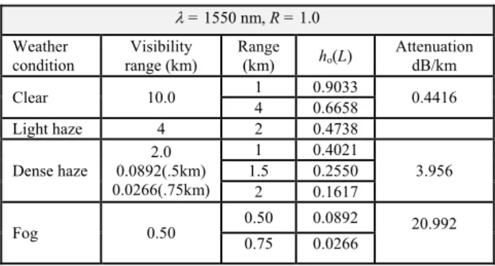
Table 1 summarizes the different weather conditions and system parameters used in this section assuming a noise standard deviation n = 10–7 A/Hz. In addition, the
following Rytov variance values: R2= 0.50, 1,0, 5.0 were
used for weak to strong turbulence channel severity. In generating the optimized results, the optimized normalized beamwidth (wza)op was found for each case of (sa ,ū, wza)
by varying the values of wza in (28) between 2 and 25.
Using (26) and (28), Figure 1 depicts minimum BER results in terms of received average SNR for weak to strong turbulence conditions and normalized jitter values
sa= 2, 3, 4. It can be concluded from the figure, that, for
any given Rytov variance and normalized jitter variance values, as the average SNR increases, optimum normalized beamwidth values increase to further minimize BER per-formance, which agrees well with the findings by [13]. In addition, for any given jitter variance and average SNR, as turbulence severity gets stronger, the value of optimum beamwidth required to achieve minimum BER results decreases.
Using (27), Figure 2 shows minimum BER perfor-mance in terms of transmitted power for weak to strong channel turbulence and light haze weather condition. The
= 1550 nm, R = 1.0 Weather
condition
Visibility range (km)
Range
(km) ho(L)
Attenuation dB/km
Clear 10.0 1 0.9033 0.4416
4 0.6658
Light haze 4 2 0.4738
Dense haze
2.0 0.0892(.5km) 0.0266(.75km)
1 0.4021 3.956 1.5 0.2550
2 0.1617
Fog 0.50 0.50 0.0892 20.992
0.75 0.0266
Fig. 1. Minimum BER results for different normalized jitter variances vs. average received SNR, .
Fig. 2. Minimum BER results for weak to strong turbulence and light haze vs. transmitted power.
results are computed for jitter variance values sa= 2, 3,
and propagation distance L = 2 km. For any given turbu-lence condition and normalized jitter variance, one can achieve possible minimum BER by adjusting the system transmitted power pt and normalized beamwidth. For
ex-ample, for R2= 1.0 and sa= 2.0, at pt = 13.0 dBm,
a minimum BER value p(e) = 2.20 × 10⁻⁸, can be achieved by adjusting the normalized beamwidth value (wza)op =7.41.
Figure 3 depicts BER results for different weather condi-tions and propagation distances. The results are computed for R2= 2.0 and sa= 3.0. It can be observed from the
figure how the BER performance is degraded due to the visibility range of the different weather conditions. As expected, the worst BER performance occurs for light fog where the visibility range is limited to 0.50 km. It is inter-esting to note, that, for any given weather conditions and propagation distance, (wza)op value that achieves minimum
p(e) is almost the same for pt ≥ 17 dBm.
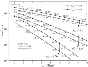
Figures 4 and 5 depict probability of outage for weak to strong turbulence conditions and normalized jitter values
sa= 2, 3, 4. It can be seen from the figures, as the value of
Fig. 3. Minimum BER results for different weather conditions and distances vs. transmitted power.
Fig. 4. Minimum outage probability for different normalized jitter variances vs. average received SNR, .
Fig. 5. Minimum outage probability for weak to strong turbulence and light haze vs. transmitted power.
average SNR or transmitted power increase, optimum normalized beamwidth values needed to achieve minimum outage probability increase, too. In addition, as the Rytov
30 35 40 45 50 55 60
10−10 10−8 10−6 10−4 10−2 100
(wza)opt= 6.29
6.65 6.80 6.85 11.62 12.03 12.23 (wza)op= 10.78
(wza)opt= 8.55
9.15
9.43
9.54
¯
u(dB)
p
(
e
)m
in
σsa= 2.0
σsa= 3.0
σsa= 4.0
σ2 R= 5.0
σ2 R= 1.0
σ2 R= 0.50
0 5 10 15 20
10−10
10−8
10−6
10−4
10−2
8.51
8.66
8.78
8.89
8.97
9.03 12.29
12.61
12.87
13.09
13.27
13.41
13.52 7.12
7.21 7.27
7.32 7.36
7.39 7.41
7.43 7.44
7.45 10.45
10.63 10.78
10.90 10.99
11.06 11.12
11.16 11.19
11.21 5.78
5.81 5.83
5.84 5.86
5.86 5.87
5.88 5.88
5.88 (wza)opt=
8.63 8.70 8.76
8.80 8.83
8.85
8.87 8.88
8.89 8.89
pt(dBm)
p
(
e
)m
in
σsa= 2.0
σsa= 3.0
σ2
R= 5.0
σ2
R= 1.0
σ2
R= 0.50 Range=2.0 km
light Haze
0 5 10 15 20
10−7 10−6 10−5 10−4 10−3 10−2 10−1
pt(dBm)
p
(
e
)min
8.63 8.88
9.08 9.25
9.38 9.49
9.57 9.63
9.68 9.71 (wza)opt=
8.11 8.44
8.73 8.96
9.15 9.31
9.43 9.52
9.59 8.94
9.14 9.29
9.42 9.51
9.59 9.64
9.69 9.72
9.74 9.29
9.42 9.51
9.59 9.64
9.69 9.72
9.74 9.76
9.77 7.73
9.57 9.63
9.68 9.71
9.74 9.76
9.77 9.78
9.79 9.43
9.52 9.59
9.65 9.69
9.72 9.74
9.76 9.77
9.78 9.14
9.29 9.42
9.51 9.59
9.64 9.69
9.72 9.74
9.76 Range=0.50 km Range=0.75 km Range=1.0 km Range=1.5 km Range=2.0 km Range=4.0 km clear weather Dense Haze light fog 9.49 σ2
R= 2.0
σsa= 3.0
30 35 40 45 50 55 60
10−8 10−7 10−6 10−5 10−4 10−3 10−2 10−1 100 ¯
u(dB)
( po u t )m in
(wza)opt= 9.70
11.17
11.84
12.14
(wza)opt= 7.38
8.70
9.24
9.47 (wza)opt= 5.01
6.25
6.65
6.80
σsa= 2.0
σsa= 3.0
σsa= 4.0
σ2 R= 0.50
σ2 R= 1.0
σ2 R= 5.0
0 2 4 6 8 10 12 14 16
10−8 10−6 10−4 10−2
pt(dBm)
(
pou
t
)min
10.77 11.05
11.27 11.44
11.56 11.66
11.73 11.78 8.463
8.30
8.58 8.66
8.73 8.78
8.82 8.84 13.10
13.53
14.15
14.36
14.53
14.67 12.59
13.87 9.892
10.19 10.44
10.63
10.78
10.90
11.00
11.07 (wza)opt=
12.05
12.42
12.74
12.99
13.19 11.59
14.56
15.31
15.95
16.48
16.91
17.27
17.55
σsa= 3.0
σsa= 4.0
σ2
R= 1.0
σ2
R= 0.50
σ2
R= 5.0
Light Haze
Fig. 6. Minimum outage probability for different weather conditions and distances vs. transmitted power.
variance moves from weak to strong turbulence strength, minimum outage probability is achieved by decreasing the laser beamwidth.
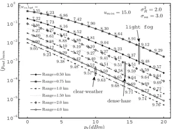
Probability of outage results for different weather conditions and propagation distances are shown in Fig. 6, using R2= 2.0 and sa= 3. The figure exhibits the same
behavior as Fig. 3, where fog weather condition highly degrades outage performance. Finally, by increasing the link operational range, minimum outage probability results are attained by adjusting the laser beamwidth to lesser values.
5.
Conclusion
In this paper, an FSO system with IM/DD and on-off signaling that operates over atmospheric slowly fading gamma-gamma turbulence channels was analyzed. Novel BER and outage probability closed form expressions are derived taking into account the combined effects of atmo-spheric turbulence, path loss due to weather conditions and pointing error. Optimized normalized beamwidth values that achieve minimum BER and outage probability were found for different SNR and transmitted power values. For each case of SNR and transmitted power, the optimized beamwidths were found by taking into account the com-bined effects of turbulence strengths, normalized jitter variance, weather condition and the length of the propaga-tion path.
As the average SNR or the transmitted power value increases, minimum BER and outage probability results are attained by increasing the laser beamwidth regardless of the jitter variance, turbulence strength and weather conditions. It was also found that increasing the path loss or moving from weak to strong turbulence channel conditions, mini-mum BER and outage probability results can be achieved by decreasing the laser beamwidth. Finally, for higher SNR and transmitted power values, optimized beamwidth values that achieve minimum BER and outage probability results are practically the same values.
References
[1] KIM, I., CHAFFEE, T., FLEISHAUER, R., et al. Advances in Communications: New FSO provides reliable 10 Gbit/s and beyond backhaul connections. Laser Focus World, 2013, p. 1-8. [2] http://www.attochron.com/
[3] KIM, I., MCARTHUR, B., KOREVAAR, E. Comparison of laser propagation at 785 nm and 1550 nm in for fog and haze for optical wireless communications. SPIE Proceedings, 2001, vol. 4214, p. 26–37. DOI: 10.1117/12.417512
[4] HASAN, O. Performance of heterodyne differential phase-shift keying system over double Weibull free-space optical channel.
Journal of Modern Optics, 2015, vol. 62, no. 11, p. 869–876. DOI: 10.1080/09500340.2015.1027311
[5] TRUNG, H., TUAN, D., PHAM, A. Pointing error effects on performance of free-space optical communication system using SC-QAM signals over atmospheric turbulence channels. AEU International Journal of Electronics and Communications, 2014, vol. 68, no. 9, p. 869–876. DOI: 10.1016/j.aeue.2014.04.008 [6] VU, B., DANG, N., THANG, T., PHAM, A. Bit error rate analysis
of rectangular QAM/FSO systems using an APD receiver over atmospheric turbulence channels. Journal of Optical Communications and Networking. 2013, vol. 5, no 5, p. 437–446. DOI: 10.1364/JOCN.5.000437
[7] MORRA, A., KHALLAF, H., SHALABY, H., KAWASAK, Z. Performance analysis of both shot- and thermal-noise limited multipulse PPM receivers in gamma–gamma atmospheric channels. Journal of Lightwave Technology, 2013, vol. 31, no. 19, p. 3142–3150. DOI: 10.1109/JLT.2013.2278692
[8] NISTAZAKES, H., TSIGOPOULOS, A., HANIAS, M., et al. Estimation of outage capacity for free space optical links over I-K and K turbulence channels. Radio Engineering, 2011, vol. 20, no. 11, p. 493–498.
[9] CHATZIDIAMANTIS, N., SANDALIDIS, H., KARAGIANNI-DIS, G., et al. New results on turbulence modeling for free-space optical systems. In Proceedings of the 17th IEEE International Conference on Telecommunications. Doha (Qatar), April, 2010. DOI: 10.1109/ICTEL.2010.5478872
[10] POPOOLA, W., GHASSEMLOOY, Z., AHMADY, V.
Performance of subcarrier modulated free-space optical communication link in negative exponential atmospheric turbulence environment. International Journal of Autonomous and Adaptive Communication Systems, 2008, vol. 1, no. 3, p. 342–355. DOI: 10.1504/IJAACS.2008.019809
[11] AL-HABASH, C., ANDREWS, L., PHILIPS, R. Mathematical model for irradiance probability density function of a laser beam propagating through turbulent media. Optical Engineering, 2001, vol. 40, no. 8, p. 1554–1563. DOI: 10.1117/1.1386641
[12] NISTAZAKIS, H., KARAGIANI, E., TSIGOPOULOS, A., et al. Average capacity of optical wireless communication systems over atmospheric turbulence channels. Journal of Lightwave Technology, 2009, vol. 27, no. 8, p. 974–979. DOI: 10.1109/JLT.2008.2005039
[13] SANDALIDIS, H., TSIFTSIS, A., KARAGIANNIS, G. Optical wireless communications with heterodyne detection over turbulence channels with pointing errors. Journal of Lightwave Technology, 2009, vol. 27, no. 20, p. 4440–4445. DOI: 10.1109/JLT.2009.2024169
[14] SANDALIDIS, H., TSIFTSIS, T. Outage probability and ergodic capacity of free-space optical links over strong turbulence.
Electronics Letters, 2008, vol. 44, no. 1, p. 46–47. DOI: 10.1049/el:20082495
[15] FARID, A., HRANILOVIC, S. Outage capacity optimization for free-space optical links with pointing errors. Journal of Lightwave Technology. 2007, vol. 25, no. 7, p. 1702–1710. DOI: 10.1109/JLT.2007.899174
0 5 10 15 20
10−6 10−5 10−4 10−3 10−2 10−1 100
7.22 7.73
8.16 8.52
8.81 9.04
9.23 9.37
9.48 9.57 (wza)opt=
6.23 6.86
7.42 7.90
8.30 8.64
8.91 9.12
9.29 8.60
8.88 9.10
9.27 9.40
9.51 9.58
9.64 9.69
9.72 8.27
8.61 8.88
9.10 9.27
9.41 9.51
9.59 9.64
9.69 7.86
8.27 8.61
8.88 9.10
9.27 9.41
9.51 9.59
9.64 9.23
9.38 9.48
9.57
9.63 9.68
9.71 9.74
9.76 8.90
9.12 9.29
9.42 9.52
9.59 9.65
9.69 9.72
9.74 5.55
pt(dBm)
(
pou
t
)min
Range=0.50 km
Range=0.75 km
Range=1.0 km
Range=1.50 km
Range=2.0 km
Range=4.0 km
light fog
9.05
densehaze clearweather
σ2
R= 2.0
σsa= 3.0
[16] SAGIAS, N., KARAGIANNIDIS, G., MATHIOPOULOS, P., et al. On the performance analysis of equal-gain diversity receiver over generalized Gamma fading channels. IEEE Transactions on Wireless Communications, 2006, vol. 5, no. 10, p. 2967–2973. DOI: 10.1109/TWC.2006.05301.
[17] Wolfram function site, http://functions.wolfram.com.
[18] ADAMCHIK, V., MARIACHEV, O. The algorithm for calculat-ing integrals of hypergeometric type and its realization in reduce system. In Proceedings of the International Symposium on Sym-bolic and Algebraic Computation (ISSAC’90). Tokyo (Japan), 1990, p. 212–224. DOI: 10.1145/96877.96930
[19] TSIFTSIS, T., SANDALIDIS, H., KARAGIANNIDIS, G., et al. Optical wireless links with diversity over strong atmospheric turbulence channels. IEEE Transactions on Wireless Communications, 2009, vol. 8, no. 2, p. 951–957. DOI: 10.1109/TWC.2009.071318
[20] KIASALEH, K. Performance of coherent DPSK free-space com-munication systems in K-distributed turbulence. IEEE Transac-tions on CommunicaTransac-tions, 2006, vol. 54, no. 4, p. 604–607. DOI: 10.1109/TCOMM.2006.873067
[21] PHILLIPS, R., ANDREWS, L. Measured statistics of laser light scattering in atmospheric turbulence. Journal of the Optical Society of America, 1981, vol. 71, no. 12, p. 1440–1445. DOI: 10.1364/JOSA.71.001440
[22] FLATTE, S., BRACHER, C., WANG, G. Probability-density functions of irradiance for waves in atmospheric turbulence calculated by numerical simulations. Journal of the Optical Society of America A, 1994, vol. 11, no. 7, p. 2080–2092. DOI: 10.1364/JOSAA.11.002080
[23] CHOUDHURY, S., GIBSON, J. D. Ergodic Capacity, Outage Capacity, and Information Transmission over Rayleigh Fading Channels. Dept. of Electrical and Computer Engineering, University of California, Santa Barbara. 5 pages. [online] Cited 2015-04-10. Available at:
http://vivonets.ece.ucsb.edu/ChoudhuryGibson_ITW07.pdf.
About the Authors ...
Omar HASAN received his B.Sc degree in Electrical
Engineering in 1987, M.Sc and Ph.D degrees in Telecommunication in 1990 and 1996, respectively, all from New Mexico State University, USA. He joined Princess Sumaya University for Technology in 1997 where he served as a chairman for the communications engineering department in the period 2005–2010 and the dean of student affairs. He worked in different projects at physical science laboratory, Las Cruces, New Mexico, USA, in the period 1991-1992. In summer 2000, he worked at Global Cardiac Monitors, research and development division in the area of Turbo coding, Webster, Texas, USA. He worked as a system analyst at Intelligent Technology Incorporated, Telecommunications division, Las Cruces, New Mexico, USA 1989-1992. He worked as a consultant for Global Cardiac Monitors LLC, Houston, Texas, USA, 2001, 2004, and 2012-current. He worked as a research assistant at the manual Lujan, Jr. center for Space and Telemetering and Telecommunications, Simulation and Tracking system division, New Mexico State University, Las Cruces, New Mexico, USA, 1996. His current research interest includes wireless optical communications and low power coding schemes. Dr. Hasan received research funding from the Higher Council for Science and Technology, development and utilization of DC and AC inverters in solar cells energy, 1999, Amman, Jordan.