ISSN 0104-6632 Printed in Brazil
www.abeq.org.br/bjche
Vol. 26, No. 01, pp. 99 - 111, January - March, 2009
Brazilian Journal
of Chemical
Engineering
INTELLIGENT TECHNIQUES FOR SYSTEM
IDENTIFICATION AND CONTROLLER
TUNING IN pH PROCESS
K. Valarmathi
1*, D. Devaraj
1and T. K. Radhakrishnan
21Department of Electrical and Electronics Engineering, Arulmigu Kalasalingam
College of Engineering, Tamilnadu, India.
E-mail: [email protected], E-mail: [email protected]
2 Department of Chemical Engineering, National Institute of Technology,
Trichy, Tamilnadu, India. E-mail: [email protected]
(Submitted: February 1, 2007 ; Revised: March 4, 2008 ; Accepted: April 21, 2008)
Abstract - This paper presents an application of Artificial Neural Network (ANN) and Genetic Algorithm (GA) for system identification for controller tuning in a pH process. In this paper, the ANN based approach is applied to estimate the system parameters. Once the variations in parameters are identified frequently, GA optimally tunes the controller. The simulation results show that the proposed intelligent technique is effective in identifying the parameters and has resulted in a minimum value of the Integral Square Error, peak overshoot and minimum settling time as compared to conventional methods. The experimental results show that their performance is superior and it matches favorably with the simulation results.
Keywords: System Identification; PID controller; Genetic Algorithm; Artificial Neural Network; pH process.
INTRODUCTION
The pH control finds wide applications in process industries. The pH process is a non-linear dynamic system and an extremely complex and challenging control problem in process industries (Kulkarni and Deshpande, 1991). The extensive applications of the pH process in industry merit the study of the control of these processes. The Proportional Integral Derivative (PID) controller has been widely used in the pH process for many years. Tuning of PID controller parameters is necessary for the satisfactory operation of the process. Traditionally, the PID controller parameters are evaluated using Ziegler-Nichols (ZN) (Astrom and Hagglund, 2001) and Cohen Coon (CC) (Schei, 1994; Shinskey, 1996) methods. In both these methods, the parameters of the controller are obtained for an operating point where the model can be considered linear. The dynamic characteristics of most of the industrial
processes exhibit nonlinear behavior and vary with time. This implies that there is sub-optimal tuning when a process operates outside the validity zone of the model. Internal Model Control (IMC) (Morari and Zufiriou, 1987) overcomes the above said problem, but its design calculations could be complicated for a higher order process.
identification methods, a model structure is selected and the parameters of the model are calculated by optimizing an objective function using an optimization technique. A variety of model structures are available to assist in modeling a system. The various models are categorized into linear and nonlinear models. The generally used linear models are Auto Regressive with eXogenous inputs (ARX), Auto Regressive with Moving Average with eXogenous inputs (ARMAX) and Output Error (OE) models. The nonlinear models include Hammerstein, Weiner model and Nonlinear Auto Regressive with Moving Average with eXogenous inputs (NARMAX). The conventional parameter identification methods namely least squares (Rad and Lo, 1997) and maximum likelihood method (Ljung, 1999) often fail in the search for a global optimum in the search space. Further, they require a large set of input/output data from the system.
Intelligent techniques overcome the difficulties and limitations encountered by the conventional approaches for system identification and controller tuning. These techniques explore the potential for creating intelligent systems by modeling the computational process of biological organisms. The constituents of this technique include Artificial Neural Network (Wasserman, 1989), Fuzzy Logic (Ross, 1995) and Genetic Algorithm (Goldberg, 1989). Narendra and Parthasarathy (1990) proposed ANN to identify the complex, nonlinear, multidimensional model. Genetic algorithm (Passino, 1996) is a general-purpose optimization algorithm based on the mechanics of natural selection and genetics. Kristinsson and Dumont (1992) proposed GA to identify plants with either minimum phase or non-minimum phase characteristic and un-modeled dynamics. Zibo and Naghdt (1995) applied genetic algorithms to identify the parameters of the Multi Input and Multi Output (MIMO) system that is assumed to have an Auto Regressive with Moving Average Exogenous (ARMAX) structure.
Lu and Basar (1995) presented the standard GA-based estimation scheme in a neural network framework, which ensure a good approximation for the system nonlinearity. Dangprasert and Avatchanakorn (1995) employed GA for on-line parameter identification and controller tuning in load frequency control of a power system. Vlachos et al. (1999) proposed a GA-based design strategy for offline PID controller tuning in linear systems. Mwembeshi and Kent (2004) proposed a GA-based Internal Model Control (IMC) strategy for a pH process. In this paper, an ANN-based approach has
been applied to estimate the changes in the parameters of the system and a GA-based approach is used to identify the optimal PID controller parameters in a pH process.
pH PROCESS
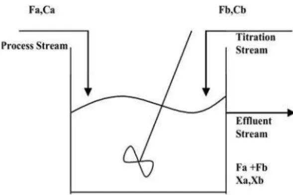
The pH is the measurement of the acidity or alkalinity of a solution. The pH process consists of neutralization of two monoprotic reagents of a weak acid (acetic acid) and a strong base (sodium hydroxide). The method implements mass balances for components called reaction invariants of the Continuous Stirred Tank Reactor (CSTR) solution. As shown in Figure 1, the CSTR has two inlet streams: the influent process stream and the titrating stream, with one effluent stream at the output. The model of the pH neutralization process used in this work follows that proposed by McAvoy et al. (1972) and is given below.
Figure 1: pH neutralization process
Assumption of perfect mixing is general in the modeling of pH processes. Material balances in the reactor can be given by
(
)
dxa
V F Ca a Fa Fb Xa
dt = − + (1)
(
)
dxb
V F C F F X
b b a b b
dt = − + (2)
whereFais the flow rate of the influent stream,Fbis
the flow rate of the titrating stream,Cais the
concentration of the influent stream,C is the b
concentration of the titrating stream, x is the a
Intelligent Techniques for System Identification and Controller Tuning in pH Process 101
concentration of the basic solution and V is the
volume of the mixture in the CSTR. The above mathematical equations describe how the concentration of the acidic and basic components,
a
x andx change dynamically with time subject to b
the input streams, F anda F . The reaction between b
HAC and NaOH:
2
H O H++OH+ (3)
HAC H++AC− (4)
NaOH Na++OH− (5)
Invoking the electroneutrality condition, the sum of the ionic charges in the solution must be zero.
[Na ] [H ] [AC ] [OH ]+ + + = − + − (6)
The [X] denotes the concentration of the X ion. The equilibrium relations also hold for water and acetic acid
[
]
a
[AC ][H ] K
HAC
− +
= (7)
whereXa =[HAC] [AC ]+ − andXb=[Na ]+ . Use of
Equations (6) and (7) gives:
3 2
a b
a b a w w a
[H ] [H ] {K X }
[H ]{K (X X ) K } K K 0
+ +
+
+ + +
− − − = (8)
Let pH= −log [H ]10 + and pKa= −log10Ka.The titration curve is given by
14
pH pH a
b pKa pH
X
X 10 10 0
1 10
−
− −
−
+ − − =
+ (9)
where KaandKwis the dissociation constant of
acetic acid at 5οC (Ka =1.778x10⁻⁵ and
14
Kw =10− ). Eq.(9) is the strictly static nonlinear
relation between the statesX ,a X and the output pH b
variable, which manifests itself as the familiar titration curve of the neutralization process.
STRATEGY FOR SYSTEM IDENTIFICATION AND CONTROLLER TUNING
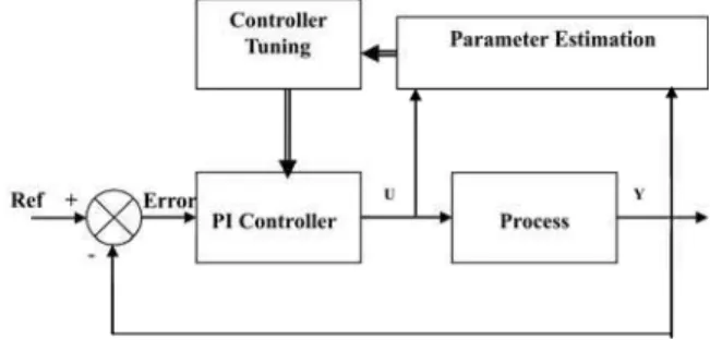
System identification is the type of experimental modeling performed for the controller design, when sufficient theoretical modeling is not available. The proposed strategy for designing the self-tuning schemes is to estimate the process parameters and to adjust the controller settings based on current parameter estimates. The block diagram representation of parameter estimation and controller tuning is shown in Figure 2.
Figure 2: ANN based Parameter Estimation and GA based Controller Tuning
Generally the parameter estimation is done using the Least Square (LS) technique. This LS estimator looks for the optimum by using the gradient technique. System identification is the prerequisite for analyzing the nonlinear process. In this paper, ANN is used for system identification. First, a suitable model of the system is selected and ANN is applied to identify the parameters of the selected model. As the plant model is identified periodically, the changes in its dynamic characteristics can be observed. Generally, for the parameter estimation, the system (G) is excited with a step function as an input, which is shown in Figure 3.
In this figure, G is an unknown system and H is an assumed model. The system parameters can be obtained by minimizing the error function e(k), where ˆy(k) is the predicted value of output based on unknown parameters and y(k) is the actual output.
The next step after system identification is the tuning of the PI controller, whose transfer function is given by
i
c p
K
G (s) K
s
= + (10)
where K is proportional gain and p K is integral i
gain. The performance of the closed loop system is defined by the performance criteria of Integral Square Error for controller (ISE(cont)), Over Shoot (OS) and Settling Time (ST) of the transient response.
The Integral Square Error squares the magnitude of error with respect to time. The overshoot is the difference between the maximum value of the output response and the steady state value and the settling time is the time for the response to stay within the specified percentage of its final value. In this work, the problem of controller tuning is formulated as an optimization problem. The objective function of the controller is to minimize the integral square error, peak overshoot, rise time and settling time of the transient response. Mathematically, this is written as
1 ISE(cont) 2 OS 3 ST
F=w F +w F +w F (11)
wherew ,1 w and 2 w are the weight factors for the 3
integral square error, overshoot and settling time respectively. The weight factors are varied between 0 and 1 to get the optimal system response. Gradient-based conventional methods are not good enough to solve this problem and a global optimization technique like genetic algorithm is well suited for this kind of problems.
DEVELOPMENT OF ANN FOR SYSTEM IDENTIFICATION
System Identification allows building mathematical models of a dynamic system based on measured data. It is done by adjusting parameters within a given model until its output coincides as much as
possible with the measured output. The assessment
of model quality is typically based on how the models perform when they attempt to reproduce the measured data.
In the identification framework, the pH process can be represented in discrete input-output form by the identification structure:
a
k b k
ˆ
ˆy[k] g[y(k 1),..., y(k n ),
u(k n ),...u(k n n 1)]
= − −
− − − + (12)
where ˆy[k] is the one-step ahead prediction of the
output, ˆg is the neural network model, u(·) are
delayed inputs to the system and na, nb, nk are system
order and delay, respectively. This is essentially a one-step ahead prediction structure in past inputs and outputs to predict the current output. The regressor structure for this network is given by:
a
k b k
ˆ ˆ
(k) [y(k 1),..., y(k n ),
u(k n ),..., u(k n n 1)]
ϕ = − −
− − − − (13)
Depending on the choice of the regression vector, different model structures emerge. At every instant, the predicted output is parameterized in terms of
network weights Θ by:
y(k, )Θ = ϕg( (k), )Θ (14)
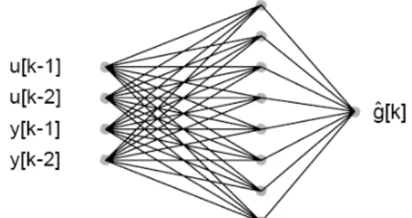
Artificial Neural Network (ANN) is used in this work for system identification. The data required to develop the ANN model for system identification are collected by conducting experiments in the laboratory grade pH process and through MATLAB simulation. The collected data is divided into training and test data. The sampling instant k is equivalent to t and the neural network structure used here is shown in Figure 4.
Figure 4: Architecture of the neural network
Intelligent Techniques for System Identification and Controller Tuning in pH Process 103 N T k 1 1 ˆ ˆ
J [y(k) y(k)] [y(k) y(k)]
2N =
=
∑
− − (15)where
e(k)= [y(k)−y(k)]ˆ (16)
Similarly, testing data are generated through the experimental setup and MATLAB simulation to minimize the cost function.
GA IMPLEMENTATION
GA has become increasingly popular in recent years in science and engineering disciplines. There are three important issues to be addressed while applying GA to solve an optimization problem:
a) Problem Representation
b) Formation of the fitness function and
c) Genetic operators
a) Problem Representation
While solving an optimization problem using GA, each individual in the population represents a candidate solution. For tuning a PID controller, the elements of the solution consist of proportional gain
(Kp) and integral gain (K ). In this work, binary i
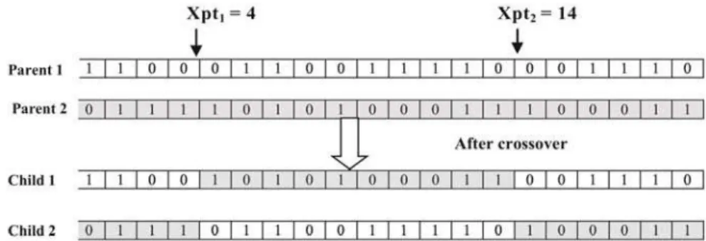
strings are used to encode the variables. A typical chromosome in the GA population for PID tuning is given below:
p i
K K
00001100 00001101
b) Formation of Fitness Function
The next important consideration is the formation of the fitness function. The performance of each individual in the population is evaluated according to its ‘fitness’, which is defined as the non-negative figure of merit to be maximized. It is associated directly with the objective function value. The values of the Integral Square Error (ISE), settling time (st) and peak overshoot (po) in Eq. (11) are calculated from the step response of the simulated system. These values are used to calculate the fitness function of the individuals.
During the GA-run, it searches for a solution with maximum fitness function value. Hence, the
minimization objective function given by (11) is transformed to a fitness function (f) to be maximized as,
f = K / F (17)
where K is a large constant. This is used to amplify (1/ F), the value of which is usually small, so that the fitness value of the chromosome will be in a wider range.
c) Genetic Operators
Figure 5: Two-point crossover
RESULTS AND DISCUSSION
This section presents the details of the development of a neural network based model for system identification and GA-based PI controller tuning for the pH process. System identification and controller tuning algorithm were evaluated on a simulated pH process. Next, the same algorithms were applied to a laboratory grade pH process. The ANN and GA code were written in MATLAB and executed on a PC with Pentium IV processor. The design details and the performance of the controller are given below.
Simulation Results
The pH process was simulated based on the Equations (1) and (2) using MATLAB Simulink. The parameters of the pH process are pH model simulated using MATLAB Simulink is shown in Figure 6. Step signal is used as the input to the system. Uniformly distributed noise is added to the step input through a uniform random generator. This is done to cause nonlinear distortion due to the dead zone nonlinearity in the pH process.
Initially, 5000 samples were generated from MATLAB simulation. 2000 samples are taken as training data set and 2800 samples are considered as
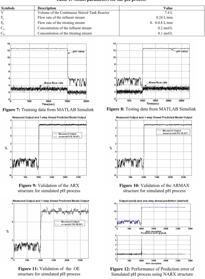
testing data set. Figure 7 and Figure 8 show the training and testing data generated using MATLAB Simulink.
Next, the different linear model structures are generated with minimization of Mean Square Error.
Figure 9 shows the ARX structure of [na nb nk] = [2 2
1], where na is equal to the number of poles and nb is
the number of zeros, while nk is the pure time-delay
in the system. Similarly, Figure 10 and Figure 11
show the ARMAX structure of [na nb nc nk] = [6 6 6
1] and OE structure of [nb nc nf] = [2 2 1], which
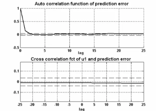
show the minimum of MSE. The conventional identification techniques cannot identify the full dynamics of the non-linear pH process. To avoid this problem, neural network based system identification is applied and the results are obtained. Figures 12-14 shows the performance of the NARX model, structure of [na nb nk] = [3 3 1]. Figure 12 illustrates
the response of prediction error and Figure 13 illustrates the auto-correlation and cross-correlation response of NARX structure. Figure 14 represents
the fitness function of MSE, which is 3.6 x 10⁻⁵.
Different structure models were checked for Mean Square Error and the results are shown in Table.2. From the Table, it is found that the NARX model structure of [3 3 1] gives the minimum MSE compared to other structures. Similarly, NARX structure of [6 6 1] of experimental data gives the minimum MSE compared to other structures.
Intelligent Techniques for System Identification and Controller Tuning in pH Process 105
Table 1: Model parameters for the pH process
Symbols Description Value
V Volume of the Continuous Stirred Tank Reactor 7.4 L
a
F Flow rate of the influent stream 0.24 L/min
b
F Flow rate of the titrating stream 0- 0-0.8 L/min
a
C Concentration of the influent stream 0.2 mol/L
b
C Concentration of the titrating stream 0.1 mol/L
Figure 7: Training data from MATLAB Simulink Figure 8: Testing data from MATLAB Simulink
Figure 9: Validation of the ARX structure for simulated pH process
Figure 10: Validation of the ARMAX structure for simulated pH process
Figure 11: Validation of the OE structure for simulated pH process
Figure 13: Auto-correlation and cross-correlation function for simulated data using NARX structure
Figure 14: Fitness curve for NARX structure
Table 2: Comparison of the Models
Model na nb nc Nf nk MSE for
Simulated data
MSE for Real data
1 1 - - 1 0.0167 0.0432
2 2 - - 1 0.0165 0.043
3 3 - - 1 0.0165 0.0432
4 4 - - 1 0.0166 0.042
ARX
6 6 - - 1 0.0166 0.039
1 1 1 - 1 0.017 0.043
2 2 2 - 1 0.017 0.039
3 3 3 - 1 0.0174 0.04
4 4 4 - 1 0.0174 0.039
ARMAX
6 6 6 - 1 0.016 0.04
- 1 1 1 - 0.061 0.169
- 2 2 1 - 0.055 0.17
- 3 3 1 - 0.059 0.18
- 4 4 1 - 0.06 0.182
OE
- 6 6 1 - 0.055 0.183
1 1 - - 1 2.2*10-4 1.74*10-2
2 2 - - 1 5.77*10-5 9.42*10-3
3 3 - - 1 3.63*10-5 9.39*10-3
4 4 - - 1 2.30*10-4 9.35*10-3
NNARX
6 6 - - 1 5.12*10-4 9.02*10-3
1 1 1 - 1 3.92*10-4 1.8*10-2
2 2 2 - 1 1.19*10-3 1.51*10-2
3 3 3 - 1 3.05*10-3 1.29*10-2
4 4 4 - 1 1.18*10-3 1.17*10-2
NNARMAX
6 6 6 - 1 2.19*10-3 1.04*10-2
From the analysis of system identification, NARX structure is [3 3 1] and the transfer
function is
2 2
0.2411Z 0.0325Z 0.08908
1 0.7814Z 0.2266Z 0.3397
+ +
− + − .
Next, the GA-based algorithm is applied to find the optimal parameters of the controller. The objective function in this case is minimization of error, peak overshoot, rise time and settle time. The optimization variables are represented as binary
Intelligent Techniques for System Identification and Controller Tuning in pH Process 107
Number of generations = 20 Population size = 10 Crossover probability = 0.8 Mutation probability = 0.08
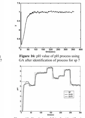
The GA took 12s to complete the 20 generations. After 20 generations it is found that all the individuals have reached almost the same fitness value. This shows that GA has reached the optimal solution. Figure 15 and Figure 16 represent the feed flow rate of acid and pH response for the set point 7. Figure 17 shows the convergence of the proposed GA algorithm. The variation of the fitness during the GA run is for the best case and shows the generation of optimal variables. It can be seen that the fitness value increases rapidly in the first 2 generations of the GA. During this stage, the GA concentrates mainly on finding feasible solutions to the problem. Then the value increases slowly and settles down near the optimum value with most of the individuals in the population reaching that point. The
performance of the various control variables in the pH process obtained through the proposed GA, compared with the performance results obtained by proposed GA and GA tuning methods for multi-stages, is shown in Figure 18.
It is clear that the proposed GA tuning produces better controller performance for the pH process, because it occupies less computation time to reach the optimal solution. For comparison, the parameters of the controller tuned using Ziegler-Nichols and Internal Model Control (IMC) methods are shown. The feed flow rate and performance of the controller using ZN and IMC for the set point of 7 are shown in Figure 19 and 20. It shows that the control performance using ZN and KT has oscillatory response and more peak overshoot and rise time is high at the set point 9. Overall the performance of the controller is found to be good when it is tuned with the proposed GA.
Figure 15: Feed flow rate of pH process using GA after identification of process for set point 7
Figure 16: pH value of pH process using GA after identification of process for sp 7
Figure 17: Convergence of GA after Identification of pH process
Figure 19: Feed flow rate of pH process using Kappa Tau and ZN tuning methods
Figure 20: Performance of pH process using Kappa Tau and ZN tuning methods
Experimental Results
In the experimental setup, acetic acid is fed to the reactor with constant flow rate and sodium hydroxide is introduced to the reactor through the pump. Figure 21 shows the pH process experimental setup. In the real time implementation, the dSPACE processor can be easily interfaced with Simulink and automatically converts the Simulink model into a targeted C code and downloads it to the designated hardware (dSPACE DS1102) via RTI. To read or write the internal variables of the control system, dSPACE Control Desk provides a user-friendly Graphic User Interface (GUI) environment that enables the user to observe vital data in the system.
From the laboratory scale pH process the feed flow rate and pH values were generated and checked with different model structures. Similar to simulated data 5000 data were generated. Figures 22 and 23 show the response of training and testing data generated experimentally. Figures 24 and 25 show
the ARX, ARMAX structures of the real data set, which matches favorably with the simulated work.
Similarly, Figures 26 and 27 show the response of the NARX structure [6 6 1] using the real dataset. Figure 26 illustrates the response of prediction error and Figure 27 shows the histogram of prediction error and parameter values. Figure 28 illustrates the auto- correlation and cross-correlation response of the NARX structure and Figure 29 represents the
fitness function of MSE, which is 9.02 x 10⁻³.
In the real time implementation, the parameters of the PI controller are fed to the pH process via MATLAB Simulink Real-Time Workshop (RTW), Real-Time Interface (RTI) and dSPACE DS1102 floating-point processor. Figures 30 and 32 represent the behavior of the base feed flow rate and pH response using conventional PI controller and show that the control performance is oscillatory. Figures 31 and 33 show the base flow rate and pH value using the GA tuned controller. From the figures, the GA tuned PI controller after identification has the minimum MSE of 0.1817.
Intelligent Techniques for System Identification and Controller Tuning in pH Process 109
Figure 22: Training data from Experimental Work
Figure 23: Testing data from Experimental Work
Figure 24: Validation of the ARX structure for Experimental work
Figure 25: Validation of the ARMAX structure for Experimental pH process
Figure 26: Performance of Prediction error of experimental pH process using
NARX structure
Figure 27: Histogram of prediction errors and linearized network parameters of experimental
Figure 28: Auto-correlation and cross-correlation function for experimental data using NARX structure
Figure 29: Fitness curve for real data using NARX structure
Figure 30: pH Response of conventional PI controller (MSE 17.01)
0 20 40 60 80 100 120 140 160 180 200
4 6 8 10 12 14 16 18 20
+20 change in acid flow rate
time(sec)
pH
v
al
ue
Figure 31: pH Response of PI controller using GA (MSE 0.1817)
0 20 40 60 80 100 120 140 160 180
0.1 0.2 0.3 0.4 0.5 0.6 0.7 0.8 0.9
+20 change in acid flow rate
time(sec)
Fb
Figure 32: Response of base flow rate using conventional PI controller
0 20 40 60 80 100 120 140 160 180 200
0.2 0.3 0.4 0.5 0.6 0.7 0.8
time(sec)
Fb
+20% change in acid flow rate
Figure 33: Response of base flow rate using GA tuned PI controller after identification
CONCLUSION
The pH control is quite difficult due to nonlinearity of the neutralization process. This process requires good control to overcome the load disturbances. This paper has demonstrated how a
Intelligent Techniques for System Identification and Controller Tuning in pH Process 111
dynamic plant characteristic changes in the pH process. Experimental results show that the proposed controller is able to tune the controller quickly and reduce the tracking error to zero, similar to simulation results.
ACKNOWLEDGEMENT
This work was performed at the Advanced Process Control Laboratory, Department of Chemical Engineering, National Institute of Technology, Trichy.
REFERENCES
Astrom, K. J. and Hagglund T., The future of PID control, Control Engineering Practice, 9, No-11, 1163–1175 (2001).
Dangprasert, P. and Avatchanakorn V., Genetic Algorithms Based Self-Tuning Regulator, IEEE International Conference on Evolutionary Computation, 1, 444-449 (1995).
Dionisio, S. and Pinto P., Genetic algorithm based system identification and PID tuning for optimum adaptive control, International Conference on Advanced Intelligent Mechatronics, California, 801-806 (2005).
Goldberg, D. E., Genetic Algorithms in Search Optimization and Machine Learning, Addison Wesley (1989).
Kristinsson, K. and Dumont G. A, System Identification and Control Using Genetic Algorithms, IEEE Trans. System, Man and Cybernetics, 22, No-5, 1033-1046 (1992).
Kulkarni, B. D. and Deshpande P. B., Nonlinear pH control, Chem. Eng. Science, 46, 995–1003 (1991).
Lennart Ljung, System Identification - Theory for the User, 2nd Ed, PTR Prentice Hall, Upper Saddle River, N. J. (1999).
Lu, S. and Basar T., Genetic algorithms-based identification, IEEE Inter. Conf. System, Man and Cybernetics, 1, 22-25 (1995).
Manfred Morari and Evanghelos Zufiriou, Robust Process Control, Prentice-Hall, NJ, 1987.
McAvoy, T. J. and Hsu, E., Dynamics of pH in Controlled Stirred Tank Reactor, Ind. Eng. Chem. Process Des. Dev., 1, No-68, 114-120 (1972). Mwembeshi, M. M. and Kent C. A., A genetic algorithm
based approach to intelligent modelling and control of pH in reactors, Computers & Chemical Engineering, 28, No-9, 1743-1757 (2004).
Narendra, K. S. and Parthasarathy K., Identification and control of dynamic systems using neural networks, IEEE Trans Neural Networks, 1, 4-27 (1990).
Passino, K. M., Towards bridging the perceived gap between conventional and intelligent control, Intelligent Control: Theory and applications, pp.1-27 (1996).
Rad, B. and Lo W.L., Self-tuning PID controller using Newton-Raphson search method, Trans. on Industrial Electronics, 44, No-5, 717-725 (1997). Schei, T. S., Automatic tuning of PID controllers
based on transfer function estimation, Automatica, 30, No-12, 1983–1989, (1994).
Shinskey, F. G., Process Control System: Application, Design and Tuning, McGraw-Hill, 4th Ed, 1996.
Timothy Ross, Fuzzy Logic with Engineering Application, Tata McGraw Hill Inc., (1995). Vlachos C., Williams D. and Gomm J. B., Genetic
approach to decentralized PI controller for multivariable processes, Proc. of IEE Control Theory Applications, 146,No-1, 58-64, (1999). Wasserman, P. D., Neural Computing: Theory and
Practice, New York, Van Nostrand Reinhold, (1989).