Cluster analysis of midlatitude oceanic cloud regimes:
mean properties and temperature sensitivity
N. D. Gordon1,*and J. R. Norris1
1Scripps Institution of Oceanography, University of California, San Diego La Jolla, CA, USA *current address: School of Earth and Environment, University of Leeds Leeds, UK
Received: 17 November 2009 – Published in Atmos. Chem. Phys. Discuss.: 20 January 2010 Revised: 16 June 2010 – Accepted: 24 June 2010 – Published: 14 July 2010
Abstract. Clouds play an important role in the climate sys-tem by reducing the amount of shortwave radiation reaching the surface and the amount of longwave radiation escaping to space. Accurate simulation of clouds in computer models re-mains elusive, however, pointing to a lack of understanding of the connection between large-scale dynamics and cloud properties. This study uses a k-means clustering algorithm to group 21 years of satellite cloud data over midlatitude oceans into seven clusters, and demonstrates that the cloud clusters are associated with distinct large-scale dynamical conditions. Three clusters correspond to low-level cloud regimes with different cloud fraction and cumuliform or stratiform char-acteristics, but all occur under large-scale descent and a rel-atively dry free troposphere. Three clusters correspond to vertically extensive cloud regimes with tops in the middle or upper troposphere, and they differ according to the strength of large-scale ascent and enhancement of tropospheric tem-perature and humidity. The final cluster is associated with a lower troposphere that is dry and an upper troposphere that is moist and experiencing weak ascent and horizontal moist advection.
Since the present balance of reflection of shortwave and absorption of longwave radiation by clouds could change as the atmosphere warms from increasing anthropogenic green-house gases, we must also better understand how increas-ing temperature modifies cloud and radiative properties. We therefore undertake an observational analysis of how mid-latitude oceanic clouds change with temperature when dy-namical processes are held constant (i.e., partial derivative with respect to temperature). For each of the seven cloud
Correspondence to: N. D. Gordon
regimes, we examine the difference in cloud and radiative properties between warm and cold subsets. To avoid misin-terpreting a cloud response to large-scale dynamical forcing as a cloud response to temperature, we require horizontal and vertical temperature advection in the warm and cold subsets to have near-median values in three layers of the troposphere. Across all of the seven clusters, we find that cloud fraction is smaller and cloud optical thickness is mostly larger for the warm subset. Cloud-top pressure is higher for the three low-level cloud regimes and lower for the cirrus regime. The net upwelling radiation flux at the top of the atmosphere is larger for the warm subset in every cluster except cirrus, and larger when averaged over all clusters. This implies that the direct response of midlatitude oceanic clouds to increasing temper-ature acts as a negative feedback on the climate system. Note that the cloud response to atmospheric dynamical changes produced by global warming, which we do not consider in this study, may differ, and the total cloud feedback may be positive.
1 Introduction
Clouds play an integral role in the climate system by reflect-ing solar radiation back to space and restrictreflect-ing the emission of terrestrial radiation to space, thereby substantially influ-encing the Earth’s temperature. For this reason, it is impor-tant to understand how clouds and their impacts on radiative transfer might respond to an initial warming from increased CO2. This is known as the cloud-climate feedback. Although
be the largest source of uncertainty in projections of future climate (IPCC, 2007).
Previous studies have used various compositing tech-niques to examine and compare how cloudiness is related to meteorological forcing in observations and models (e.g., Klein and Jakob, 1999; Norris and Weaver, 2001; Tselioudis and Jakob, 2002). Dividing the atmosphere into a series of distinct meteorological regimes, each with different cloud properties, is an effective method for understanding the con-nections between the dynamics and thermodynamics of the atmosphere and the clouds they produce (Jakob, 2003). More recent investigations have used clustering algorithms to more objectively identify cloud regimes without direct reference to meteorological parameters (e.g., Jakob and Tselioudis, 2003; Gordon et al., 2005; Jakob et al., 2005; Rossow et al., 2005). Williams and Tselioudis (2007) examined differences be-tween simulated cloud properties in control runs and 2×CO2
experiments through the use of a clustering algorithm. Identi-fying the specific vertical distribution of dynamical and ther-modynamical processes generating a particular type of cloud is crucial for understanding the atmosphere and improving model simulation of clouds.
The present study extends the clustering approach of Gor-don et al. (2005) to all midlatitude ocean grid boxes, where clouds have a very large impact on shortwave radiation (Weaver and Ramanathan, 1997). Only ocean regions are ex-amined so as to minimize the role that surface features play in cloud forcing. We use ak-means clustering algorithm to clas-sify daily grid box cloud data from the International Satellite Cloud Climatology Project (ISCCP) into seven groups ac-cording to similar cloud fraction values in three cloud-top pressure intervals and three cloud optical thickness intervals. Vertical profiles of reanalysis relative humidity, temperature, vertical velocity, horizontal temperature advection, and hor-izontal moisture advection are averaged over each cluster as perturbations from the mean state. This provides insight into meteorological conditions and dynamical forcing associated with each cloud regime, which is supplemented by examina-tion of the climatological distribuexamina-tion and seasonal cycle of each cluster.
Since current global climate models do not provide reli-able information on the cloud response to global warming (e.g., Ringer et al., 2006; Clement et al., 2009; among oth-ers), we will additionally use our clustering analysis as a foundation for investigation of the sensitivity of cloud prop-erties to changes in temperature. To avoid the confound-ing effects of dynamical processes that can influence both temperature and clouds, we investigate how cloud properties vary with temperature within a narrow range of dynamical parameters, following the approach of Bony et al. (2004). Clustering is a useful tool for this purpose because it groups cloud types with similar meteorology, and Williams and Tse-lioudis (2007) employed it to examine the relative contribu-tion of changes to cloud properties due to dynamic and ther-modynamic changes in GCMs. In the present study, each
cluster is divided into relatively warm and cold subsets. The impact of joint dynamical forcing on temperature and cloudi-ness is removed by restricting warm and cold subsets to have near-median values of horizontal and vertical temperature advection and near-median values of lapse rate in the lower troposphere and tropopause region. The difference between cold and warm subsets provides information on how large-scale cloud and radiative properties are affected by increas-ing temperature directly rather than through changes in atmo-spheric circulation associated with global warming. These results will give insight into cloud feedback on the climate system and be a useful baseline for model evaluation.
2 Data sources
The source of cloud observations for this investigation was the three-hourly International Satellite Cloud Clima-tology Project (ISCCP) D1 equal-area (280 km×280 km) data set, originally processed from radiances primarily mea-sured by geostationary weather satellites (Rossow et al., 1996; Rossow and Schiffer, 1999). The ISCCP data con-sist of cloud fractions within a grid box for nine categories of cloudiness based on three intervals of cloud-top pres-sure (CTP) (below 680 mb, between 680 and 440 mb, and above 440 mb) and three intervals of cloud optical thickness (τ ) (between 0.3 and 3.6, between 3.6 and 23, and above 23). Satellite pixels used to generate the CTP-τ histograms are approximately 4–7 km in size and spaced approximately 30 km apart, with up to 80 pixels per grid box. Since cloud optical thickness values are obtained from visible retrievals, valid data only exist for daytime hours. We restricted our analysis to one time point per day for each satellite grid box, choosing the value with the smallest solar-zenith angle (clos-est to local noon). This r(clos-estriction avoided sampling biases associated with more valid data points coming from regions near the equator and from points in the summer hemisphere, where there are a greater number of daylight hours.
Additional quality control included removal of all grid box values with any sea ice, as reported by the satellite, or any points with anomalously high clear-sky albedo (αclear). The
normal range ofαclearwas determined for bins of solar-zenith
angle (SZA) by calculating the difference between the first percentile and the median value. For each SZA bin, all data for whichαclearvalues were greater than the sum of the
me-dian and the difference between the meme-dian and the first per-centile value were excluded. This assumes that validαclear
varies uniformly above and below the median. We also ex-cluded data for which satellite skin temperature (Tskin)was
less than 271 K, more than 4 K colder than NCEP reanaly-sis SST, or more than 8 K warmer than reanalyreanaly-sis SST. As noted by Tsuang et al. (their Fig. 3, 2008), Tskin tended to
thus enabling a comprehensive investigation of the cloud re-sponse to temperature when large-scale dynamical condi-tions are held constant. The CTP-τ histogram corresponds to a type cloud fraction array. All values of the nine-type cloud fraction array are exactly zero for clear-sky obser-vations, which infrequently occur (less than 1% of the total number of days and grid boxes) and are excluded from the clustering. To complement the satellite-derived properties of the cloud regimes, we also analyzed surface-based visual cloud type observations from the Extended Edited Cloud Re-port Archive (EECRA) (Hahn and Warren, 1999).
In addition to mean cloud properties, we examined the three-hourly radiative flux data derived from the ISCCP data (Zhang et al., 2004). The flux data consists of upwelling and downwelling, shortwave and longwave radiative flux for both clear and cloudy parts of the grid box. This data is pro-vided at the surface, the top of the atmosphere (TOA), and at three levels within the atmosphere (680 mbar, 440 mbar, and 100 mbar). While the uncertainties of instantaneous flux val-ues are on the order of 10 Wm2, these will be considerably reduced in the clusters by averaging over a large number of values. While systematic biases may exist in ISCCP FD data due to satellite changes, we do not expect them to produce substantial differences between cloud clusters.
Since our selection of the one satellite observation per day that is closest to local noon would otherwise produce a sub-stantial radiative bias, we divided near-noon upwelling TOA SW fluxes by near-noon insolation to convert them to values of reflectivity. Reflectivity values were multiplied by diur-nal mean insolation to convert them back to diurdiur-nal mean upwelling SW flux (more details are available in Appendix A). This procedure assumes that systematic cloud changes near local noon are characteristic of the entire day. Aver-aging diurnal mean flux values across different grid boxes and seasons gives more radiative weighting to cloud changes that occur at lower latitudes and during the summer season. While this may be more relevant to the overall impact on cli-mate, in the present study we are more interested in the typi-cal cloud response to increasing temperature. For this reason we gave equal weighting to clouds in all grid boxes and sea-sons by separately averaging reflectivity values and diurnal mean insolation values before multiplying them together to obtain average diurnal mean upwelling flux. Our results are qualitatively the same irrespective of radiative weighting.
We obtained information about the dynamics and thermo-dynamic structure of the atmosphere from the National Cen-ter for Environmental Prediction (NCEP) NCAR Reanalysis
the satellite grid boxes. Moreover, vertical motion at mid-dle latitudes is better constrained via quasi-geostrophic re-lationships by satellite and radiosonde observations of tem-perature and horizontal wind. Although deficiencies exist in the dynamics as represented in reanalyses (Trenberth et al., 2001), the accuracy of the NCEP Reanalysis in the midlati-tudes is greatly improved in the model satellite era, post 1978 (Bromwich and Fogt, 2004). Additionally, our main interest is in the relationship between dynamics and cloud properties, and Norris and Weaver (2001) found negligible differences between cloud-vertical motion relationships when using the NCEP and ECMWF Reanalyses.
3 Cluster analysis method
The ISCCP cloud data were grouped into regimes by apply-ing a k-means clustering algorithm to the nine-type cloud fraction arrays (CTP-τ histograms). Thek-means procedure classifies all nine-type arrays into a specified number of clus-ters such that within-cluster variance is minimized (Hartigan, 1975; Jakob and Tselioudis, 2003). The only arbitrary pa-rameter needed is the number of clusters; the character of the individual cluster means is then objectively determined by the data. The clustering process began with random se-lection ofktype arrays as initial seeds. All other nine-type arrays in the data set were then assigned to the initial seed to which they were closest in a Euclidean sense. The number of nine-type arrays in a cluster divided by the total number of nine-type arrays is the frequency of occurrence of the cluster, and the average of all nine-type arrays in the cluster is the centroid (i.e., average cloud fraction for each of the nine CTP-τ categories). These cluster centroids be-came new seeds to reinitialize the clustering routine, which was repeated until the centroids converged.
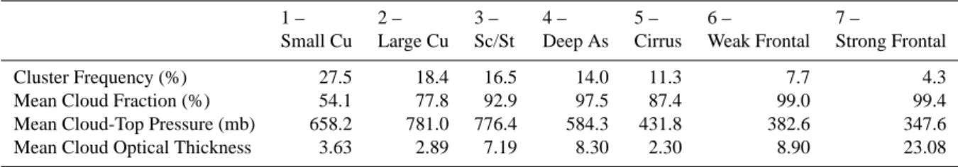
Table 1. Grid box mean ISCCP cloud properties for each cluster.
1 – 2 – 3 – 4 – 5 – 6 – 7 –
Small Cu Large Cu Sc/St Deep As Cirrus Weak Frontal Strong Frontal
Cluster Frequency (%) 27.5 18.4 16.5 14.0 11.3 7.7 4.3 Mean Cloud Fraction (%) 54.1 77.8 92.9 97.5 87.4 99.0 99.4 Mean Cloud-Top Pressure (mb) 658.2 781.0 776.4 584.3 431.8 382.6 347.6 Mean Cloud Optical Thickness 3.63 2.89 7.19 8.30 2.30 8.90 23.08
preceding clusters without providing appreciable new infor-mation; inclusion of such intermediate clusters would have increased the number of plots without commensurately en-hancing our understanding of dynamical and thermodynami-cal conditions associated with particular cloud regimes.
Our approach differs from that of Gordon et al. (2005) in that we cluster on cloud fraction in nine CTP-τ categories rather than grid box mean cloud fraction, cloud-top pressure, and cloud reflectivity. We instead took the approach used by Jakob and Tselioudis (2003), except that they used 42 CTP-τ
categories (cloud fraction within each of seven CTP and sixτ
intervals). Because cloud fraction in 42 CTP-τ categories did not provide significantly more information, we aggregated the 42 categories into nine categories that correspond to the standard ISCCP-defined cloud types.
4 Cloud properties
Table 1 lists mean cloud fraction, CTP andτ averaged over all CTP-τ categories for the cluster centroids during the 1984–2004 time period, ordered according to relative fre-quency. The nonlinear relationship between radiation flux and optical thickness was taken into account by convert-ing cloud optical thickness values to cloud reflectivity at 0.6 microns using an ISCCP look-up table (corresponding to Fig. 3.13 in Rossow et al., 1996) before averaging. The mean reflectivity was then converted back to cloud optical thickness using the same table. This ensures that our cluster mean optical thickness values more correctly represent cloud effects on grid box mean visible radiation flux.
Table 2 lists mean TOA shortwave cloud radiative forcing (SWCRF) and longwave cloud radiative forcing (LWCRF) for each of the clusters. These are diurnal mean values calculated from near-noon values according to the method described in the Appendix. Following Charlock and Ra-manathan (1985), we define cloud radiative forcing as outgo-ing radiative flux for all-sky conditions subtracted from out-going radiative flux for cloud-free conditions. Thus, SWCRF values are negative and represent a net cooling of the climate system, and LWCRF values are positive and represent a net warming of the climate system. Reasons for the informal
names given to each cluster in Tables 1 and 2 will be de-scribed in the following paragraphs.
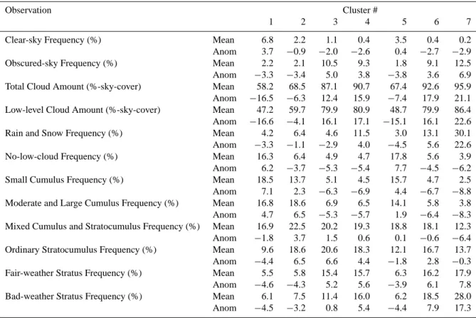
As a complement to the satellite observations, we ex-amined cloud information reported by surface observers on ships in the same grid box and on the same day as the IS-CCP data. These provide a bottom-up view of the scene along with morphological rather than radiative characteriza-tions of cloud types as well as precipitation (see Table 1 of Norris, 1998a). Table 3 lists average surface-observed total cloud cover and low-level cloud cover for each cluster to-gether with the frequencies at which surface observers report the occurrence of clear sky, sky obscuration by fog or pre-cipitation, non-drizzle prepre-cipitation, various low-level cloud types, and the absence of low-level cloudiness. In order to distinguish relative differences between clusters more eas-ily, anomalies from the frequency-weighted mean across all clusters are provided. Because ship sampling is sparse over southern hemisphere midlatitude oceans, Table 3 includes only northern hemisphere points. This should not bias the results appreciably since no cluster is primarily restricted to the southern hemisphere, and mean cloud properties and dy-namics are similar for each cluster in either hemisphere (not shown). There is general agreement but not exact correspon-dence between Table 1 and Table 3 due to the different spatial scale and method of satellite and surface observations.
0.3 3.6 23 378 1000
Cloud−Top Pressure (mb)
0.16
0.05 0.1
0.3 3.6 23 378 1000
0.43
0.05 0.1
0.3 3.6 23 378 1000
0.62
0.05 0.1
0.3 3.6 23 378
1000 0.05
0.1
0.3 3.6 23 378 30
440
680
1000
Cluster 5
Optical Depth
Cloud−Top Pressure (mb)
0.38
0.05 0.1 0.15 0.2 0.25 0.3
0.3 3.6 23 378 30
440
680
1000
Cluster 6
Optical Depth 0.54
0.05 0.1 0.15 0.2 0.25 0.3
0.3 3.6 23 378 30
440
680
1000
Cluster 7
Optical Depth 0.56
0.05 0.1 0.15 0.2 0.25 0.3
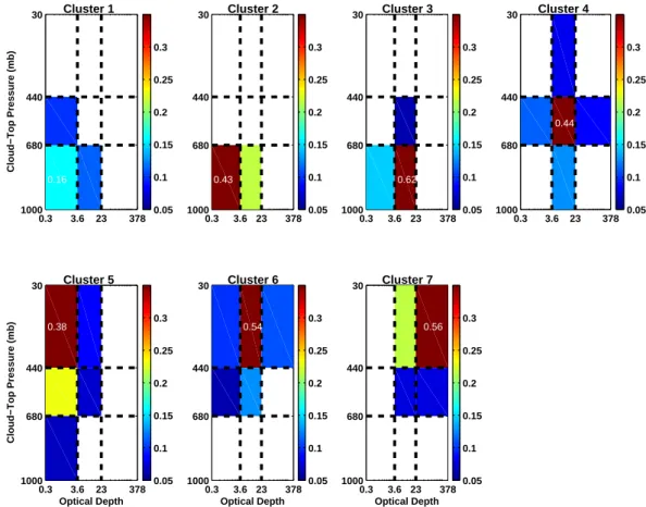
Fig. 1. Mean ISCCP histograms of cloud fraction for each cloud-top pressure and cloud optical thickness interval.
Table 2. Grid box mean ISCCP cloud radiative forcing for each cluster.
1 – 2 – 3 – 4 – 5 – 6 – 7 –
Small Cu Large Cu Sc/St Deep As Cirrus Weak Frontal Strong Frontal
SWCRF (Wm2) −39.01 −40.46 −96.96 −112.89 −55.04 −123.05 −168.38 LWCRF (Wm2) 14.81 10.32 13.17 40.59 46.71 78.26 87.02
Cluster 4 is the only cluster with a cloud top in the mid-dle troposphere (Fig. 1). The large low-level cloud amount and stratiform cloud types very frequently reported by sur-face observers for this cluster (Table 3) suggest that these clouds usually extend from the middle troposphere down to near the surface, even though the satellite retrievals are unable to provide that information. For this reason, we call Cluster 4 “deep altostratus”. Table 2 shows that it has larger LWCRF than the low-level cloud clusters and rela-tively strong SWCRF.
The last three clusters in Fig. 1 are high-top cloud regimes with optical thickness that increases from Cluster 5 to 6 to 7. We call Cluster 5 “cirrus” because it has the smallest optical thickness and least low-level cloud of all clusters (Tables 1 and 3). The magnitude of SWCRF is only slightly larger than
Table 3. Mean surface-reported cloud properties for each cluster (northern hemisphere only), along with anomaly from the average over all clusters.
Observation Cluster #
1 2 3 4 5 6 7
Clear-sky Frequency (%) Mean 6.8 2.2 1.1 0.4 3.5 0.4 0.2 Anom 3.7 −0.9 −2.0 −2.6 0.4 −2.7 −2.9 Obscured-sky Frequency (%) Mean 2.2 2.1 10.5 9.3 1.8 9.1 12.5 Anom −3.3 −3.4 5.0 3.8 −3.8 3.6 6.9 Total Cloud Amount (%-sky-cover) Mean 58.2 68.5 87.1 90.7 67.4 92.6 95.9 Anom −16.5 −6.3 12.4 15.9 −7.4 17.9 21.1 Low-level Cloud Amount (%-sky-cover) Mean 47.2 59.7 79.9 80.9 48.7 79.9 86.4 Anom −16.6 −4.1 16.1 17.1 −15.1 16.1 22.6 Rain and Snow Frequency (%) Mean 4.2 6.4 4.6 11.5 3.0 13.1 30.1 Anom −3.3 −1.1 −2.9 4.0 −4.5 5.6 22.6 No-low-cloud Frequency (%) Mean 16.3 6.4 4.9 4.7 17.8 5.6 3.9 Anom 6.2 −3.7 −5.3 −5.4 7.7 −4.5 −6.2 Small Cumulus Frequency (%) Mean 18.5 13.7 5.1 4.5 15.7 4.7 2.5 Anom 7.1 2.3 −6.3 −6.9 4.4 −6.7 −8.8 Moderate and Large Cumulus Frequency (%) Mean 16.8 18.6 6.9 6.5 14.1 5.8 3.8 Anom 4.7 6.5 −5.3 −5.7 1.9 −6.4 −8.3 Mixed Cumulus and Stratocumulus Frequency (%) Mean 16.9 22.5 20.2 19.3 18.8 18.1 12.3 Anom −1.8 3.7 1.5 0.6 0.1 −0.6 −6.4 Ordinary Stratocumulus Frequency (%) Mean 9.6 18.6 20.6 18.3 12.1 16.7 13.7 Anom −4.4 6.5 6.6 4.4 −1.8 2.8 −0.3 Fair-weather Stratus Frequency (%) Mean 5.5 5.8 15.4 15.7 6.3 16.2 17.9 Anom −4.6 −4.3 5.2 5.6 −3.9 6.1 7.8 Bad-weather Stratus Frequency (%) Mean 6.1 7.5 11.4 16.0 6.2 18.5 28.0 Anom −4.5 −3.2 0.8 5.4 −4.4 7.9 17.3
−70 Wm2value reported by Weaver and Ramanathan (1996) for midlatitude ocean synoptic storms. Averaging over all clusters with weighting by their relative frequencies, we cal-culate a net CRF cooling of−39 Wm2by midlatitude ocean clouds.
As mentioned previously, our clustering algorithm may converge to a different solution, depending on the initial seeds provided. We resolved this by taking the solution with the smallest total variance. Besides the solution presented in Fig. 1, there are two additional sets of clusters to which the solution can converge. The only difference is the inclusion of either another low-level cloud or midlevel cloud cluster, both of which occur with the loss of one of the frontal clus-ters. In analyzing clustering results for values ofk greater than seven, we often found cases with more than three low-level cloud clusters or more than one midlow-level cloud clus-ter. In both of these instances, the inclusion of the additional cluster did not provide any additional information since the cluster with intermediate cloud properties also exhibited termediate meteorological properties. Clustering analysis in-dependently applied to individual ocean basins and seasons produced types similar to those described above, albeit with possibly different frequencies.
5 Characteristic dynamics
−10 0 10 20 30 800
900
1000
%
−10 0 10 20 30 800
900
1000
%
−10 0 10 20 30 800
900
1000
%
−10 0 10 20 30 800
900
1000
%
−10 0 10 20 30 100
200
300
400
500
600
700
800
900
1000
%
Pressure
Cluster 5
−10 0 10 20 30 100
200
300
400
500
600
700
800
900
1000
%
Cluster 6
−10 0 10 20 30 100
200
300
400
500
600
700
800
900
1000
%
Cluster 7
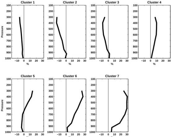
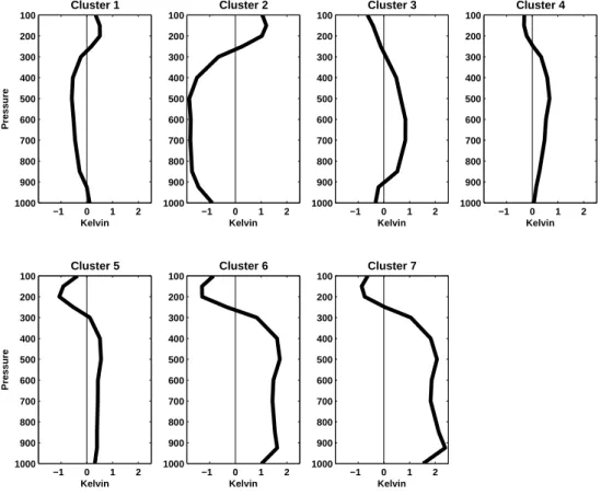
Fig. 2. Vertical profiles of mean perturbation relative humidity for each cluster from the NCEP Reanalysis.
of temperature in Fig. 6. Profiles of vertical advection ten-dencies of both temperature and water vapor (not shown) are similar to the profile of vertical motion (water vapor being the opposite sign). We have not included bars corresponding to the 95% confidence interval on either side of the profiles because, in nearly every instance, the uncertainty range was indistinguishable from the mean profile (due to the very large number of data points contributing to each cluster).
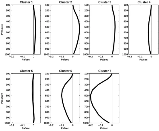
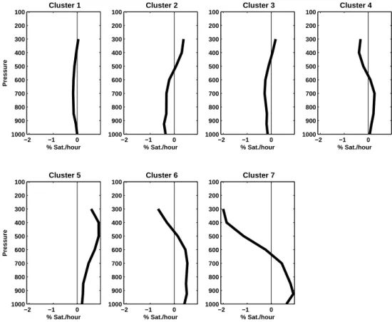
The mean cloud properties of each cluster are physically consistent with the meteorological state and dynamical forc-ing. The low-level cloud Clusters (1, 2, and 3) occur with negative perturbation RH in the middle and upper tropo-sphere (Fig. 2) that is produced by grid box mean vertical de-scent (Fig. 4). Cluster 1 (Small Cu) has the weakest average dynamical forcing, with near-mean profiles in temperature (Fig. 3), zonal and meridional wind (not shown), horizontal advection of moisture (Fig. 5), and horizontal advection of temperature (Fig. 6). Clusters 2 and 3 have similar dynamics (downward motion and low-level horizontal advective pertur-bation drying and cooling), but their temperature profiles are quite different. Cluster 2 (Large Cu) occurs with a relatively cold boundary layer and cold free troposphere, whereas Clus-ter 3 (Sc/St) occurs with a relatively cool boundary layer and relatively warm free troposphere (thus indicating a perturba-tion temperature inversion). These characteristics are
con-sistent with the vertical temperature profile and dynamical processes previously found to be associated with surface-observed midlatitude large cumulus and stratocumulus, re-spectively (Norris, 1998a; Norris and Klein, 2000). In the Large Cu cluster, perturbation temperature switches from cold below 300 mb to warm above 300 mb, suggesting a de-pressed tropopause. Contrastingly, the Sc/St cluster has an opposite temperature reversal – warm below and cold above 300 mb, suggesting a slightly elevated tropopause (Fig. 3).
−1 0 1 2 100
200
300
400
500
600
700
800
900
1000
Kelvin
Pressure
Cluster 1
−1 0 1 2 100
200
300
400
500
600
700
800
900
1000
Kelvin
Cluster 2
−1 0 1 2 100
200
300
400
500
600
700
800
900
1000
Kelvin
Cluster 3
−1 0 1 2 100
200
300
400
500
600
700
800
900
1000
Kelvin
Cluster 4
−1 0 1 2 100
200
300
400
500
600
700
800
900
1000
Kelvin
Pressure
Cluster 5
−1 0 1 2 100
200
300
400
500
600
700
800
900
1000
Kelvin
Cluster 6
−1 0 1 2 100
200
300
400
500
600
700
800
900
1000
Kelvin
Cluster 7
Fig. 3. As in Fig. 2, except for perturbation temperature.
Cluster 4 (Deep As) exhibits vertical profiles of perturba-tion RH, temperature, vertical velocity, horizontal temper-ature advection, and horizontal moisture advection that have similar shapes and signs, albeit with much weaker magni-tude, to those of the frontal clusters.
The RH profile for Cluster 5 (Cirrus) shows negative turbation moisture below 600 mb and significant positive per-turbation moisture above 600 mb (Fig. 2), and the negative temperature perturbation above 250 mb (Fig. 3) suggests that it coincides with an elevated tropopause. The large positive horizontal perturbation moisture advection (Fig. 5) suggests that some of these clouds are blow-off from a deep convec-tive system or an extratropical cyclone, and the small upward motion in the upper troposphere suggests that some of these clouds may be locally dynamically generated (Fig. 4).
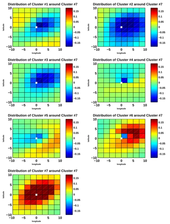
In addition to looking at the local meteorological con-ditions, we can examine the spatial relationships between cloud regimes corresponding to each cluster. This can be accomplished by compositing the frequency of occurrence of various clusters in grid boxes surrounding a central point (e.g., Lau and Crane, 1995; Norris and Iacobellis, 2005). In this case we choose as a central point those grid boxes in which the Strong Frontal cluster is present. To avoid biases from geographical and seasonal variations in cluster distri-bution, we subtracted the long-term monthly mean cluster
frequency for each grid box before adding it to the compos-ite. Figure 7 shows the results, which are generally consis-tent with the placement of cloud regimes in a midlatitude synoptic wave. Points located in the Southern Hemisphere have been inverted before averaging so that the figure is dis-played in a Northern Hemisphere sense, namely the bottom of the domain is towards the equator. By construction, there is a large positive perturbation in the frequency of Cluster 7 (Strong Frontal) at the center of the composite. Similar to Lau and Crane (1995), who composited on points of high optical thickness, Cluster 7 frequency is preferentially ori-ented in a SW-NE fashion (in a northern hemisphere sense). Cluster 6 (Weak Frontal) is also relatively frequent in the re-gion surrounding the center, especially to the northeast (in a northern hemisphere sense). The frequency of Cluster 5 (Cirrus) is enhanced equatorward and eastward (i.e., ahead) of the frontal regime. Clusters 1 (Small Cu) and 2 (Large Cu) more frequently occur northwest of the frontal regime (i.e., in the cold sector).
6 Spatial distribution and seasonal cycle
−0.2 −0.1 0 800
900
1000
Pa/sec
−0.2 −0.1 0 800
900
1000
Pa/sec
−0.2 −0.1 0 800
900
1000
Pa/sec
−0.2 −0.1 0 800
900
1000
Pa/sec
−0.2 −0.1 0 100
200
300
400
500
600
700
800
900
1000
Pa/sec
Pressure
Cluster 5
−0.2 −0.1 0 100
200
300
400
500
600
700
800
900
1000
Pa/sec
Cluster 6
−0.2 −0.1 0 100
200
300
400
500
600
700
800
900
1000
Pa/sec
Cluster 7
Fig. 4. As in Fig. 2, except for perturbation pressure vertical velocity.
satellites are present and do not reflect real geographical vari-ations (Rossow and Garder, 1993). The overall most frequent cluster, Small Cu, predominantly occurs in equatorward and coastal regions of our domain (Fig. 8a), as may be expected for the cluster with the least cloud fraction and greatest preva-lence of surface-reported cumuliform cloud types (Table 3 of this study; Figs. 5 and 6 of Norris, 1998b). The
CTP-τ histogram for Small Cu (Fig. 1) shows that this cluster is primarily composed of low-level clouds, but some small amount of higher clouds is mixed in, as implied by the lower grid box mean CTP for this cluster relative to the other low-level cloud clusters (Table 1). The second cluster, Large Cu, occurs more often in the center of the ocean basins and is more prevalent in the southern hemisphere (Fig. 8b). The fi-nal low-level cloud cluster, Sc/St, has a very distinctive geo-graphical distribution. The region of highest frequency is the subtropical anticyclone region in the eastern Pacific Ocean, and other regions of frequent Sc/St include the far northern Pacific Ocean and off the west coast of Australia (Fig. 8c). Other climatological subtropical stratocumulus regions are too far equatorward to be included in our analysis (Norris, 1998b).
The only predominantly midlevel cluster, Deep As, is pri-marily located in the higher latitude regions of the analysis domain (Fig. 8d). Cluster 5 (Cirrus) is most frequent im-mediately east of continents (South America, North
Amer-ica, and southern Africa). Another region of increased fre-quency is in the central Pacific, possibly due to advection from the deep convective towers of the west Pacific equato-rial warm pool (Fig. 8e). The final two clusters (Weak Frontal and Strong Frontal) are fixtures of the storm track, with the Strong Frontal cluster more focused in the western half of the ocean basins (Fig. 8f–g).
Williams and Tselioudis (2007) (hereafter WT07) per-formed a similar study by clustering ISCCP histograms for the ice-free extratropics (poleward of 20◦ in both hemi-spheres). Although they only examine five cloud clusters, their results are very similar to those produced from our anal-ysis (Fig. 6 from WT07). The WT07 clusters of shallow cu-mulus, stratocucu-mulus, cirrus, mid-level, and frontal are sim-ilar to Small Cu, Sc/St, Cirrus, Deep As, and Strong Frontal (respectively). The WT07 study examined a much larger do-main, allowing points poleward of 55◦, provided that they are
June-July-−2 −1 0 100
200
300
400
500
600
700
800
900
1000
% Sat./hour
Pressure
Cluster 1
−2 −1 0 100
200
300
400
500
600
700
800
900
1000
% Sat./hour
Cluster 2
−2 −1 0 100
200
300
400
500
600
700
800
900
1000
% Sat./hour
Cluster 3
−2 −1 0 100
200
300
400
500
600
700
800
900
1000
% Sat./hour
Cluster 4
−2 −1 0 100
200
300
400
500
600
700
800
900
1000
% Sat./hour
Pressure
Cluster 5
−2 −1 0 100
200
300
400
500
600
700
800
900
1000
% Sat./hour
Cluster 6
−2 −1 0 100
200
300
400
500
600
700
800
900
1000
% Sat./hour
Cluster 7
Fig. 5. As in Fig. 2, except for perturbation horizontal moisture advection.
August (JJA) seasons, respectively. This cloud regime pre-dominantly occurs in the winter season, suggesting that these clouds are the result of cold air advecting over warmer water behind a frontal system (Fig. 7). Cluster 3 (Sc/St) also has a very strong seasonal cycle (Fig. 10a–b), but unlike Cluster 2, it primarily occurs during the summer season. Stratocu-mulus clouds in the eastern Pacific anticyclone region and stratus clouds in the central North Pacific are most extensive during JJA (Norris, 1998b).
The spatial distribution of Cluster 4 (Deep As) frequency for each season is fairly similar to the mean distribution (not shown). One large exception is the North Pacific during JJA, where Deep As is especially prevalent (Fig. 11). The re-striction of this cloud regime to higher latitudes and its in-creased frequency in northern hemisphere summer suggests that these are weakly forced and shallow synoptic storms. Surface observers report precipitation for the Deep As clus-ter nearly as often as they do for the Weak Frontal clusclus-ter (Table 3). Cluster 5 (Cirrus) also has little seasonality for the most part. One exception is that the frequency of Cirrus is en-hanced in the western North Pacific Ocean near the southern boundary of our domain during JJA (Fig. 12). These high-level clouds may be the result of greater nearby convection in the western tropical warm pool.
7 Temperature sensitivty analysis method
0 0.2 0.4 800
900
1000
K/hour
0 0.2 0.4 800
900
1000
K/hour
0 0.2 0.4 800
900
1000
K/hour
0 0.2 0.4 800
900
1000
K/hour
0 0.2 0.4 100
200
300
400
500
600
700
800
900
1000
K/hour
Pressure
Cluster 5
0 0.2 0.4 100
200
300
400
500
600
700
800
900
1000
K/hour
Cluster 6
0 0.2 0.4 100
200
300
400
500
600
700
800
900
1000
K/hour
Cluster 7
Fig. 6. As in Fig. 2, except for perturbation horizontal temperature advection.
and vertical temperature advection. This is conducted inde-pendently for three different layers of the atmosphere, which corresponded to the layers of the ISCCP cloud histograms (1000–680 mb, 680–440 mb, and 440–100 mb). Examining warm-cold differences in cloud properties only for conditions of median advection minimizes the possibility of misinter-preting a cloud-temperature relationship produced by large-scale dynamics for a thermodynamic response. Such confu-sion could arise because variability in cloud amount, temper-ature, advection, and the storm track are closely connected over midlatitude oceans (Norris, 2000).
Two more meteorological conditions that we restricted were lower-tropospheric static stability (LTS) and the tropopause height. The former has particular influence on low-level cloud properties (Klein and Hartmann, 1993; Nor-ris, 1998), while the latter primarily affects the high-cloud clusters. Because advection over the ocean produces a greater change in temperature in the mid-troposphere than near the surface, warm cases are on average associated with stronger stability than cold cases. To minimize the confound-ing influence of changes in LTS on cloud-temperature re-lationships, we required that the temperature difference be-tween 1000 mb and 70 mb be bebe-tween the 25th and 75th per-centiles. For the high-cloud clusters, warm cases tend to oc-cur with a higher tropopause, which allows clouds to extend
to greater elevation. To minimize this effect, we required that the temperature difference between 200 mb and 400 mb be between the 25th and 75th percentiles (thus constraining variations in tropopause height). These restrictions were ap-plied independently to each ISCCP grid box, calendar month, and cluster number with an equal number of warm and cold cases retained. Although midlatitude lapse rate will probably decrease with global warming, albeit much less so than in the tropics (Fig. 10.7 of IPCC, 2007), we did not attempt to re-produce this in differences between warm and cold cases be-cause that would have required complicated additional com-posite restrictions,
Our division of the initial 10 million daily grid box obser-vations into warm and cold subsets for conditions of median advection and lapse rate in three layers of the troposphere left us with about 75 000 observations designated as warm and an equal number as cold. Since the warm and cold observations were uniformly distributed geographically and seasonally in proportion to cluster frequency, our results are globally rep-resentative of clouds over midlatitude oceans. Assuming that observations are independent if they are not in adjacent grid boxes and separated by more than one day in time, the effec-tive number of observations,Neff, is about 1/4 of the nominal
−10 −5 0 5 10 −10
−5 0 5 10
longitude
latitude
Distribution of Cluster #1 around Cluster #7
−0.15 −0.1 −0.05 0 0.05 0.1 0.15
−10 −5 0 5 10
−10 −5 0 5 10
longitude
latitude
Distribution of Cluster #2 around Cluster #7
−0.15 −0.1 −0.05 0 0.05 0.1 0.15
−10 −5 0 5 10
−10 −5 0 5 10
longitude
latitude
Distribution of Cluster #3 around Cluster #7
−0.15 −0.1 −0.05 0 0.05 0.1 0.15
−10 −5 0 5 10
−10 −5 0 5 10
longitude
latitude
Distribution of Cluster #4 around Cluster #7
−0.15 −0.1 −0.05 0 0.05 0.1 0.15
−10 −5 0 5 10
−10 −5 0 5 10
longitude
latitude
Distribution of Cluster #5 around Cluster #7
−0.15 −0.1 −0.05 0 0.05 0.1 0.15
−10 −5 0 5 10
−10 −5 0 5 10
longitude
latitude
Distribution of Cluster #6 around Cluster #7
−0.15 −0.1 −0.05 0 0.05 0.1 0.15
−10 −5 0 5 10
−10 −5 0 5 10
longitude
latitude
Distribution of Cluster #7 around Cluster #7
−0.15 −0.1 −0.05 0 0.05 0.1 0.15
Fig. 7. Composite spatial distributions of the perturbation frequency of each cluster around a central grid box with the Strong Frontal cluster.
8 Impact of increasing temperature on cloud properties
Since we are interested in how cloud properties change with increasing tropospheric temperature, we examined differ-ences between the warm and cold cases. Figure 13 shows IS-CCP CTP-τ histograms for the average warm minus cold dif-ference in cloud fraction for each of the seven clusters. Un-shaded areas of the histograms represent regions where the difference was not significant at the 95% confidence level.
We calculated confidence levels using a bootstrap method wherein two sets ofNeffvalues were randomly selected from
0 50 100 150 200 250 300 350 −60
−40 −20 0
0.05 0.1 0.15
0 50 100 150 200 250 300 350
−60 −40 −20 0
0.05 0.1 0.15
0 50 100 150 200 250 300 350
−60 −40 −20 0 20 40 60 (c)
0.05 0.1 0.15 0.2 0.25 0.3
0 50 100 150 200 250 300 350
−60 −40 −20 0 20 40 60 (d)
0.05 0.1 0.15 0.2 0.25 0.3
Fig. 8. Annual mean climatological spatial distributions of the frequency of each cluster, (a) Small Cumulus, (b) Large Cumulus, (c) Stratocumulus/Stratus, (d) Deep Altostratus, (e) Cirrus, (f) Weak Frontal, and (g) Strong Frontal.
temperature. Those differences that are different from zero at the 95% confidence level are displayed in bold in Table 4. We used an ISCCP look-up table (corresponding to Fig. 3.13 in Rossow et al., 1996) to convert visible cloud optical thick-ness to infrared window cloud emissivity.
Figure 13 and Table 4 show a generally consistent reduc-tion in cloud fracreduc-tion, increase in cloud-top pressure (low-ering of cloud top), and increase in optical thickness across all clusters for increasing temperature. Cluster 1 (Small Cu) exhibits the largest decrease in cloud fraction at−2.3% K−1,
accompanied by increases in cloud-top pressure and optical thickness. The other low-level cloud clusters (Large Cu and Sc/St) have smaller reductions in cloud fraction and larger increases in cloud-top pressure (+6.9 and+9.1 mb K−1, re-spectively). The enhancement of optical thickness for the small Cu and Large Cu clusters (+0.13K−1and+0.09 K−1, respectively) is produced by a decrease in the occurrence of
optically thin clouds and an increase in the occurrence of optically thick clouds within the grid box (Fig. 13). Clus-ter 3 (Sc/St) is the only clusClus-ter with a reduction in optical thickness for increasing temperature (−0.05 K−1), which is due to a decrease in the occurrence of optically thick clouds (Fig. 13).
Cluster 4 (Deep As) shows little change in cloud fraction or cloud-top pressure but has the largest change in optical thickness (+0.33 K−1), as seen in Table 4. The latter is
produced by a decrease in the occurrence of optically thin clouds and an increase in the occurrence of optically thick clouds (Fig. 13). Cluster 5 (Cirrus) exhibits a reduction in cloud fraction (−0.9% K−1), and it is the only cluster with a substantial decrease in cloud-top pressure (−3.8 mb K−1)
0 50 100 150 200 250 300 350 −60
−40 −20 0 20 40 60 (e)
0.05 0.1 0.15 0.2 0.25 0.3
0 50 100 150 200 250 300 350
−60 −40 −20 0 20 40 60 (f)
0.05 0.1 0.15 0.2 0.25 0.3
0 50 100 150 200 250 300 350
−60 −40 −20 0 20 40 60 (g)
0.02 0.04 0.06 0.08 0.1 0.12 0.14 0.16 0.18 0.2
Fig. 8. Continued.
+0.25 K−1due to the more frequent occurrence of optically thick clouds. The strong frontal cluster exhibits no signifi-cant changes with increasing temperature (Table 4).
Although there is substantial noise due to small sample sizes for individual grid boxes, the geographical and seasonal distributions of differences in cloud properties between warm and cold subsets for a given cluster appear to be uniform (not shown). This suggests that the information in Table 4 repre-sents the general response of various cloud regimes to warm-ing rather than a particular response driven by a change only in one region or season.
To provide context for how cloud properties change with temperature, we present the average vertical profiles of me-teorological parameters derived from NCEP Reanalysis for the warm and cold subsets of each cluster. Figure 14 shows the vertical profiles of temperature anomalies with respect to grid box and calendar month means. By construction,
0 50 100 150 200 250 300 350 −60
−40 −20 0
0.05 0.1 0.15
0 50 100 150 200 250 300 350
−60 −40 −20 0
0.05 0.1 0.15
Fig. 9. Seasonal mean climatological spatial distributions of the frequency of Cluster 2 (Large Cumulus), (a) DJF and (b) JJA.
0 50 100 150 200 250 300 350
−60 −40 −20 0 20 40 60 (a)
0.05 0.1 0.15 0.2 0.25 0.3
0 50 100 150 200 250 300 350
−60 −40 −20 0 20 40 60 (b)
0.05 0.1 0.15 0.2 0.25 0.3
Fig. 10. As in Fig. 9, except for Cluster 3 (Stratocumulus/Stratus), (a) DJF and (b) JJA.
a large influence over midlatitude ocean cloudiness (Lau and Crane, 1995; Norris and Klein, 2000; Weaver and Ra-manathan, 1997), and Fig. 17 shows that vertical profiles of vertical velocity anomalies are almost exactly the same for warm and cold subsets. This result gives us confidence that our restriction of temperature advection to near-median val-ues successfully eliminated differences in the large-scale dy-namical forcing of clouds in the warm and cold subsets of each cluster.
9 Impact of increasing temperature on radiative properties
Table 4. Average cloud properties for the entire cluster, warm subset, cold subset, and the difference between the two divided by the temperature change for each cluster (Subsets different at the 95% confidence level are in bold).
1 – 2 – 3 – 4 – 5 – 6 – 7 –
Small Cu Large Cu Sc/St Deep As Ci Weak Frontal Strong Frontal
Cluster Frequency (%) 27.5 18.4 16.5 14.0 11.3 7.7 4.3 Warm – Cold Difference (K) 2.25 2.23 2.25 2.58 2.37 2.45 2.37 Cluster Cloud Fraction (%) 54.1 77.8 92.9 97.5 87.4 99.0 99.4 Warm Subset (%) 45.5 75.8 92.0 97.7 85.0 99.3 99.5 Cold Subset (%) 50.7 77.1 92.9 97.9 87.0 99.4 99.5 Difference (% K−1) −2.3 −0.6 −0.4 −0.1 −0.9 0.0 0.0 Cluster CTP (mb) 658.2 781.0 776.4 584.3 431.8 382.6 347.6 Warm Subset (mb) 679.2 799.2 795.0 588.1 425.2 389.1 350.9 Cold Subset (mb) 668.7 783.8 774.5 589.5 434.1 388.5 349.0 Difference (mb K−1) +4.6 +6.9 +9.1 −0.5 −3.8 +0.3 +0.8 Cluster Optical Thickness 3.63 2.89 7.19 8.30 2.30 8.90 23.08 Warm Subset 3.32 2.89 7.07 8.30 2.12 9.06 22.63 Cold Subset 3.03 2.69 7.19 7.46 2.06 8.44 22.63 Difference (K−1) +0.13 +0.09 −0.05 +0.33 +0.03 +0.25 0.00 Cluster Emissivity 0.835 0.823 0.979 0.985 0.776 0.993 1.000 Warm Subset 0.825 0.823 0.979 0.986 0.750 0.994 1.000 Cold Subset 0.802 0.805 0.978 0.981 0.746 0.992 1.000 Difference (K−1) +0.010 +0.008 0.000 +0.002 +0.002 +0.001 0.000
Table 5. Average total SWCRF, SWCRF from cloud fraction change, and SWCRF from albedo change for entire the cluster, warm subset, cold subset, and the difference between the two (per degree temperature change; Subsets different at the 95% confidence level are in bold).
1 – 2 – 3 – 4 – 5 – 6 – 7 –
Small Cu Large Cu Sc/St Deep As Ci Weak Frontal Strong Frontal
Cluster Total SWCRF (Wm−2) −39.0 −40.5 −97.0 −112.9 −55.0 −123.1 −168.4 Warm Subset (Wm−2) −30.8 −38.8 −93.9 −113.1 −51.1 −125.2 −167.1 Cold Subset (Wm−2) −32.3 −38.5 −96.6 −109.3 −51.8 −122.6 −167.2 Difference (Wm−2K−1) +0.7 −0.2 +1.2 −1.5 +0.3 −1.1 +0.1 SWCRFCF
Warm Subset (Wm−2) −25.7 −36.7 −95.3 −111.13 −47.3 −117.3 −162.8 Cold Subset (Wm−2) −28.6 −37.3 −96.3 −111.35 −48.5 −117.4 −162.8 Difference (Wm−2) +1.3 +0.3 +0.5 +0.1 +0.5 +0.1 0.0 SWCRFalbedo
Warm Subset (Wm−2) −27.5 −37.4 −95.0 −113.2 −48.0 −118.7 −162.7 Cold Subset (Wm−2) −26.8 −36.5 −96.6 −109.3 −47.9 −116.1 −162.8 Difference (Wm−2) −0.3 −0.4 +0.7 −1.5 0.0 −1.1 +0.1
SWCRF= −f αSW↓TOA (1)
α=αovercast−αclear=
SW↑TOAovercast−SW↑TOAclear
SW↓TOA (2)
wheref is cloud fraction andαis the difference between the albedo of an overcast scene and the clear-sky albedo. Albedo values were obtained by dividing TOA upwelling SW flux by insolation. For all clusters, the changes to clear-sky albedo are smaller than the changes to the albedo of the overcast
scene (Table 5). The individual impacts of cloud fraction and albedo changes on SWCRF are defined as follows.
1SWCRFCF= −1f αSW↓TOA (3)
1SWCRFα= −f 1αSW↓TOA (4)
where the overbar indicates the cluster average.1SWCRFCF
0 50 100 150 200 250 300 350 −60
−40 −20
0.05 0.1 0.15
Fig. 11. JJA mean climatological spatial distribution of the fre-quency of Cluster 4 (Deep Altostratus).
by the average cluster albedo and diurnal insolation, and
1SWCRFα represents the modification in SWCRF resulting from the warm minus cold difference in albedo multiplied by average cluster cloud fraction and diurnal insolation. The fact that the sum of1SWCRFCF and1SWCRFα is nearly the same as the total change in SWCRF indicates that, within a particular cloud regime, there is little correlation between variability in cloud fraction and variability in cloud albedo. All calculations are conducted such that a positive number represents a net radiative warming of the climate system for an increase in temperature.
For Cluster 1 (Small Cu), the radiative warming associ-ated with a reduction in cloud fraction is only partially bal-anced by a radiative cooling associated with a small increase in albedo/optical thickness, resulting in a total SW radiative warming of+0.7 Wm−2K−1(Tables 4 and 5). For Cluster 2 (Large Cu), the small radiative warming due to a decrease in cloud fraction is contrastingly more than compensated for by the radiative cooling from the increased optical thickness of these clouds (total SW radiative cooling is−0.2 Wm−2
K−1). The reductions in cloud fraction and optical
thick-ness with increasing temperature for Cluster 3 (Sc/St) both contribute to SW radiative warming (total is +1.2 Wm−2 K−1). Clusters 4 and 6 (Deep As and Weak Frontal) have the greatest differences in total SW radiative cooling (−1.5 and−1.1 Wm−2 K−1, respectively), both of which are the result of the increase in cloud optical thickness, but Cluster 7 (Strong Frontal) experiences very little change in SWCRF because its extensive and optically thick clouds are near ra-diative saturation. The SW rara-diative warming of+0.3 Wm−2 K−1for Cluster 5 (Cirrus) primarily results from the reduc-tion of cloud fracreduc-tion, while changes in optical thickness have small impact.
0 50 100 150 200 250 300 350
−60 −40 −20
0.05 0.1 0.15
Fig. 12. As in Fig. 11, except for Cluster 5 (Cirrus).
Our observational method is not a suitable analogue for the global warming scenario when calculating the difference between the average LWCRF for the warm and cold subsets. This is because tropospheric temperature differences are sub-stantially larger than surface temperature differences in our analysis (i.e., daily temperature variability is larger for the troposphere than for the ocean surface), unlike the more uni-form surface and atmospheric warming expected from a dou-bling of CO2(IPCC, 2007). Because LW emission is
sensi-tive to temperature, our observational analysis will underesti-mate the upwelling LW flux from the surface relative to what will happen during future climate change and thus produce biased LWCRF. Despite our inability to quantify the total LW radiative change between warm and cold subsets, we can nonetheless examine changes in components of LWCRF, de-fined here as the product of cloud fraction and the difference between upwelling TOA clear-sky and overcast LW flux. LWCRF=f (LW↑TOAclear−LW↑TOAovercast) (5) Overcast LW flux is defined as follows,
LW↑TOAovercast=(1−gac)[εσ TCT4 +(1−ε)LW↑bc] (6)
wheregac is the above-cloud greenhouse parameter,εis the
cloud emissivity,σis the Stefan-Boltzmann constant,TCTis
the temperature at cloud top, and LW↑bc is the upwelling
LW flux coming from beneath the cloud. Overcast refers to the flux that would occur if the entire scene were filled with clouds. We will not consider how LWCRF may be af-fected by changes in clear-sky LW flux in the present anal-ysis, which has the advantage of avoiding possible disagree-ment between the sign of the CRF change and the sign of the cloud feedback that was noted by Soden et al. (2008).
0.3 3.6 23 378 30
440
680
1000
Cloud−Top Pressure (mb)
Cluster 1
0.02
−0.02 −0.01 0 0.01 0.02
0.3 3.6 23 378 30
440
680
1000
Cluster 2
0.01
−0.02 −0.01 0 0.01 0.02
0.3 3.6 23 378 30
440
680
1000
Cluster 3
0.01
−0.02 −0.01 0 0.01 0.02
0.3 3.6 23 378 30
440
680
1000
Cluster 4
0.03
−0.02 −0.01 0 0.01 0.02
0.3 3.6 23 378 30
440
680
1000
Optical Depth
Cloud−Top Pressure (mb)
Cluster 5
0.02
−0.02 −0.01 0 0.01 0.02
0.3 3.6 23 378 30
440
680
1000
Optical Depth
Cluster 6
0.02
−0.02 −0.01 0 0.01 0.02
0.3 3.6 23 378 30
440
680
1000
Optical Depth
Cluster 7
0
−0.02 −0.01 0 0.01 0.02
Fig. 13. ISCCP histograms of difference in cloud fraction between warm and cold subsets for each cluster.
cloud top level and the top of the atmosphere. It is simi-lar to the greenhouse parameter devised by Raval and Ra-manathan (1989) and Cess and Udelhofen (2003), except that instead of accounting for the ratio in surface and TOA LW flux, we are interested in the ratio of cloud level and TOA LW flux. The upwelling flux at cloud level is composed of thermal emission by the cloud as well as a portion of LW flux from below transmitted through the cloud. For cloud regimes that have near-unit emissivity, namely Sc/St, Deep As, Weak Frontal, and Strong Frontal, the transmission of below-cloud LW flux will be negligible. Using values of TOA overcast LW flux and TCT (Table 1), we calculated averagegac for
those four clusters withε≈1. Figure 18 demonstrates that
gac varies nearly linearly with cloud-top pressure (i.e.,
in-versely with atmospheric mass above the cloud top). Assum-ing that this is the only factor controllAssum-inggac, we interpolate
the values in Fig. 18 to the average cloud-top pressures of the remaining clusters to obtaingacfor those clusters withε <1.
With these estimates for the fraction of upwelling radiation absorbed by the atmosphere above the cloud for each cluster, we can use Equation 6 to calculate the below-cloud LW flux for the three clusters withε <1 (Table 6).
Using cluster average values of LW flux that do not suf-fer from disproportionate changes in tropospheric and sur-face temperature, we can calculate the individual impacts of
changes in cloud fraction, cloud emissivity, and cloud-top pressure on LWCRF:
1LWCRFCF=1f (LW↑TOAclear−LW↑TOAovercast) (7)
1LWCRFε= −f (1−gac)1ε[σ T 4
CT−LW↑bc] (8)
1LWCRFCTP= −f (1−gac)[4εσ T 3
CTdT /dp1pCT] (9)
As before, the overbar indicates cluster averages and the
1indicates the difference between warm and cold subsets. The change in cloud-top pressure1pCTwas converted to a
change in cloud-top temperature using cluster average lapse rate from the NCEP reanalysis. Values for 1LWCRFCF, 1LWCRFε, and 1LWCRFCTP are displayed in Table 7.
−2 0 2 4 800
900
1000
K
−2 0 2 4 800
900
1000
K
−2 0 2 4 800
900
1000
K
−2 0 2 4 800
900
1000
K
−2 0 2 4 100
200
300
400
500
600
700
800
900
1000
K
Pressure
Cluster 5
−2 0 2 4 100
200
300
400
500
600
700
800
900
1000
K
Cluster 6
−2 0 2 4 100
200
300
400
500
600
700
800
900
1000
K
Cluster 7
Fig. 14. Vertical profiles of temperature anomalies for warm (red) and cold (blue) subsets for each cluster from the NCEP reanalysis.
Table 6. Below-cloud upwelling LW flux.
1 – 2 – 5 – Small Cu Large Cu Cirrus
Cluster LWbc(Wm−2) 305.0 357.7 338.0
The three low-level clusters exhibit a lowering of cloud top, leading to greater LW emission and a negative change in LWCRF, but the Cirrus cluster shows a rising cloud top, lead-ing to less LW emission and a positive change in LWCRF.
Assuming that variations in cloud fraction, cloud emissiv-ity, and cloud-top pressure are uncorrelated within each clus-ter, we can sum their individual contributions to LWCRF to obtain an approximation of the total LWCRF change asso-ciated with the difference between the warm and cold sub-sets. These are listed in Table 8, and indicate that the Cir-rus cluster (+1.0 Wm−2K−1)has the largest positive change in LWCRF for increasing temperature, corresponding to a warming effect on the climate system. The other clusters exhibit either a weakly positive or largely negative change (near zero to−1.5 Wm−2K−1). For the low-level clusters, the summed LW radiative cooling values are larger than any
of the total SW radiative heating values, resulting in net ra-diative cooling for all low-level cloud regimes (−0.4,−0.9, and−0.3 Wm−2K−1for Small Cu, Large Cu, and Sc/St, re-spectively). The net radiative cooling for the low-level cloud regimes results from a reduction in greenhouse effect due to lower mean cloud top height and less cloud cover that is larger than the reduction in solar reflection due to less cloud cover. LW radiative changes are very small for the Deep As and Weak Frontal clusters, and SW radiative cooling due to enhanced optical thickness dominates to produce net radia-tive cooling for these cloud regimes (−1.1 and−1.0 Wm−2 K−1for Deep As and Weak Frontal, respectively). LW, SW, and net radiative effects are small for the Strong Frontal cloud regime, and Cirrus is the only cloud regime for which there is both LW and SW radiative warming for increasing temperature (net value is+1.3 Wm−2K−1). The only
−0.2 0 0.2 100
200
300
400
500
600
700
800
900
1000
Pressure
Cluster 1
−0.2 0 0.2 100
200
300
400
500
600
700
800
900
1000
Cluster 2
−0.2 0 0.2 100
200
300
400
500
600
700
800
900
1000
Cluster 3
−0.2 0 0.2 100
200
300
400
500
600
700
800
900
1000
Cluster 4
−0.2 0 0.2 100
200
300
400
500
600
700
800
900
1000
Pressure
Cluster 5
−0.2 0 0.2 100
200
300
400
500
600
700
800
900
1000
Cluster 6
−0.2 0 0.2 100
200
300
400
500
600
700
800
900
1000
Cluster 7
Fig. 15. As in Fig. 14, except for relative humidity anomalies.
Table 7. Average LWCRF from cloud fraction change, LWCRF from emissivity change, and LWCRF from cloud-top pressure change for the difference between the warm and cold subsets (per degree temperature change; Subsets different at the 95% confidence level are in bold).
1 – 2 – 3 – 4 – 5 – 6 – 7 –
Small Cu Large Cu Sc/St Deep As Cirrus Weak Frontal Strong Frontal
1LWCRFCF(Wm−2K−1) −0.6 −0.1 −0.1 0.0 −0.5 0.0 0.0 1LWCRFε(Wm−2K−1) +0.1 +0.3 0.0 +0.2 +0.4 +0.2 0.0
1LWCRFCTT(Wm−2K−1) −0.5 −0.9 −1.4 +0.1 +1.1 −0.1 −0.3
10 Discussion
The broad results of the preceding analysis suggest that a warmer troposphere promotes reduced cloud fraction, en-hanced cloud optical thickness, a lower cloud top for low-level clouds, and a higher cloud top for cirrus over the mid-latitude ocean. Since this study was constructed to eliminate variations in temperature associated with horizontal and ver-tical advection along with variations in lapse rate, we pre-sume that the observed changes are directly connected to in-creased temperature rather than large-scale dynamical pro-cesses. The reduction in cloud fraction with warmer temper-ature is consistent with the findings of previous investigations of cloud-temperature relationships over midlatitude oceans (Norris and Leovy, 1994; Weare, 1994; Norris and
Iacobel-lis, 2005; Wagner et al., 2008), but the enhancement of cloud optical thickness may not be. Williams and Webb (2009), using a clustering routine to examine the response of GCM-simulated cloud regimes to a doubling of CO2, found that
most models produced a shift towards optically thicker low-level clouds and more elevated high-low-level clouds with warm-ing in the ice-free extratropics.
0 1 2 800
900
1000
g/kg
0 1 2 800
900
1000
g/kg
0 1 2 800
900
1000
g/kg
0 1 2 800
900
1000
g/kg
0 1 2 100
200
300
400
500
600
700
800
900
1000
g/kg
Pressure
Cluster 5
0 1 2 100
200
300
400
500
600
700
800
900
1000
g/kg
Cluster 6
0 1 2 100
200
300
400
500
600
700
800
900
1000
g/kg
Cluster 7
Fig. 16. As in Fig. 14, except for specific humidity anomalies.
Table 8. Total SWCRF and sum of LWCRF component changes for each cluster and the average from the midlatitude based on relative frequency of occurrence. (Subsets different at the 95% confidence level are in bold).
1 – 2 – 3 – 4 – 5 – 6 – 7 – Midlatitude Small Cu Large Cu Sc/St Deep As Cirrus Weak Frontal Strong Frontal Ocean Average
Cluster Frequency 27.5 18.4 16.5 14.0 11.3 7.7 4.3 (%)
Sum of LWCRF components −1.1 −0.7 −1.5 +0.3 +1.0 +0.1 −0.3 (Wm−2K−1)
Total SWCRF +0.7 −0.2 +1.2 −1.5 +0.3 −1.1 +0.1 (Wm−2K−1)
Net CRF −0.4 −0.9 −0.3 −1.1 +1.3 −1.0 −0.3 −0.5 (Wm−2K−1)
(Mitchell et al., 1989). Contrastingly, previous observational work using the same satellite cloud dataset as in this study in-dicates that cloud optical thickness decreases with tempera-ture over the midlatitude North Pacific (Norris and Iacobellis, 2005). Tselioudis et al. (1992) also reported a decrease in op-tical thickness with temperature for midlatitude oceanic low-level clouds warmer than -10◦C, even when partially cloud-filled pixel effects are taken into account (Chang and Coak-ley, 2007). Two of the low-level cloud clusters examined in this study (Small Cu and Large Cu) exhibit an increase in