doi:10.5194/bg-8-147-2011
© Author(s) 2011. CC Attribution 3.0 License.
Spatial and temporal variation of CO
2
efflux along a disturbance
gradient in a miombo woodland in Western Zambia
L. Merbold1,4, W. Ziegler1, M. M. Mukelabai2, and W. L. Kutsch3
1Max-Planck Institute for Biogeochemistry, P.O. Box 100164, 07701 Jena, Germany
2Zambia Meteorological Department, Haile Sellasie Avenue, City Airport, P. O. Box 30200, 10101 Lusaka, Zambia 3Johann Heinrich von Th¨unen Institut (vTI), Institute for Agricultural Climate Research, Bundesallee 50,
38116 Braunschweig, Germany
4Institute of Agricultural Sciences, Grassland Science Group, ETH Zurich, Universit¨atsstrasse 2, 8092 Zurich, Switzerland
Received: 4 May 2010 – Published in Biogeosciences Discuss.: 29 July 2010
Revised: 7 December 2010 – Accepted: 17 December 2010 – Published: 21 January 2011
Abstract. Carbon dioxide efflux from the soil surface was
measured over a period of several weeks within a hetero-geneous Brachystegia spp. dominated miombo woodland in Western Zambia. The objectives were to examine spatial and temporal variation of soil respiration along a disturbance gra-dient from a protected forest reserve to a cut, burned, and grazed area outside, and to relate the flux to various abiotic and biotic drivers. The highest daily mean fluxes (around 12 µmol CO2m−2s−1)were measured in the protected
for-est in the wet season and lowfor-est daily mean fluxes (around 1 µmol CO2m−2s−1)in the most disturbed area during the
dry season. Diurnal variation of soil respiration was closely correlated with soil temperature. The combination of soil water content and soil temperature was found to be the main driving factor at seasonal time scale. There was a 75% de-crease in soil CO2 efflux during the dry season and a 20%
difference in peak soil respiratory flux measured in 2008 and 2009. Spatial variation of CO2efflux was positively related
to total soil carbon content in the undisturbed area but not at the disturbed site. Coefficients of variation of efflux rates between plots decreased towards the core zone of the pro-tected forest reserve. Normalized soil respiration values did not vary significantly along the disturbance gradient. Spatial variation of respiration did not show a clear distinction be-tween the disturbed and undisturbed sites and could not be explained by variables such as leaf area index. In contrast, within plot variability of soil respiration was explained by soil organic carbon content.
Correspondence to: L. Merbold ([email protected])
Three different approaches to calculate total ecosystem respiration (Reco)from eddy covariance measurements were
compared to two bottom-up estimates ofRecoobtained from
chambers measurements of soil- and leaf respiration which differed in the consideration of spatial heterogeneity. The consideration of spatial variability resulted only in small changes of Reco when compared to simple averaging.
To-tal ecosystem respiration at the plot scale, obtained by eddy covariance differed by up to 25% in relation to values cal-culated from the soil- and leaf chamber efflux measurements but without showing a clear trend.
1 Introduction
Soil respiration is the major path by which carbon dioxide (CO2)returns to the atmosphere after being fixed via
photo-synthesis by land plants. Globally this flux is estimated to be approximately 75 Pg C per year, or 10 times the emissions originating from fossil fuel combustion, and is likely to be affected by anthropogenic global warming (Schlesinger and Andrews, 2000; Bond-Lamberty and Thomson, 2010). The large amount of carbon cycled via respiration notwithstand-ing the prediction of soil CO2efflux at all scales remains one
of the big challenges in biogeochemistry, since soil respira-tion represents a combinarespira-tion of different sources, each with its own response to environmental factors and each with its own temporal variability and spatial heterogeneity (Bahn et al., 2009; Trumbore, 2006).
1998). Spatial patterns in soil carbon dioxide efflux have shown to be associated with heterogeneity of soil properties such as soil organic matter content or microbial biomass, but also have been explained by stand aboveground species com-position and structure (Soe and Buchmann, 2005; Shibistova et al., 2002, 2002b; Knohl et al., 2008).
Measurements of soil- and ecosystem CO2 fluxes have
been made in a wide variety of ecosystems, especially forest and agricultural ecosystems in America and Europe (Borken et al., 2002; Hanson et al., 2003), but there is a paucity of similar studies from tropical ecosystems particularly in Africa (Nouvellon et al., 2008). Up to date, there is not a single study of continuous ecosystem flux measurements nor regular process measurements representing miombo wood-lands, the most extensive (2.7 mio km2) semi-arid to sub-humid woodland formation in Southern Africa (Kanschik and Becker, 2001; Grace et al., 2006).
Miombo woodlands are the current location of the tropical deforestation and forest degradation front. The main driver is charcoal production to satisfy a growing energy demand in regional urban areas (Misana et al., 2005). After cutting for charcoal, the land is often cultivated as cropland, grazed or burned. In these cases the belowground carbon stocks in miombo woodlands are substantially reduced (Walker and Desanker, 2004; Chidumayo and Kwibisa, 2003; Zingore et al., 2005).
Knowledge about the sources of heterogeneity is essen-tial for scaling soil respiration from plot measurements to ecosystem, landscape or even global level (Soegaard et al., 2000; Tang and Baldocchi, 2005). In this context, it is a great advantage that studies on the heterogeneity of soil CO2efflux
can be conducted within the footprint area of flux towers and the up-scaled values of soil respiration can be compared to integrated fluxes from eddy covariance (EC) night-time data (Janssens et al., 2000; Aubinet et al., 2005; Kutsch et al., 2010). Night time measurements of carbon dioxide fluxes by EC represent the total ecosystem respiration (Reco)which
also includes stem- and foliar respiration. Therefore, the comparison of up-scaled soil respiration toRecorequires an
estimation of these fluxes originating from the aboveground part of the ecosystem.
In this study, we investigate the spatial and temporal drivers of soil respiration, and to compare “top-down” (eddy covariance) and “bottom-up” (chambers) methods of esti-mating ecosystem respiration (1). Specifically, we aim to investigate (i) soil respiration, in view of hourly up to yearly periods, (ii) spatially at scales of meters to hundreds of me-ters, and (iii) the abiotic and biotic factors that drive this het-erogeneity. In particular (iv), we wanted to know whether information of small scale heterogeneity becomes irrelevant during scaling and whether further efforts of scaling soil res-piration can be conducted by reduced sampling.
The second (2) main objective of our work was to study the impact of disturbance. We used a gradient from a pro-tected forest reserve to a human-disturbed derivative as an
0 - 45 °
N
prevailing wind direction (east south-east) 50 m
EC Tower
1
2
3
disturbed
undisturbed
4
Plot with categorized subplots (100 each)
8
0
-
1
2
5
°
12
5
1
40
°
140 - 1 80 °
distur
banc
e g
radien
t
soil r
espir
a
tion and car
bon c
on
ten
t?
soil w
a
ter c
on
ten
t?
leaf ar
ea inde
x?
soil t
emper
a
tur
e?
char
coal c
on
ten
t?
Fig. 1. Scheme of the site and experimental setup in Mongu
(Zam-bia). The dark grey area represents the disturbed area driven by de-forestation, burning and grazing. The light grey area represents the north western corner of Kataba forest reserve, established in 1973. The measurement plots, divided into subplots of different ground cover, were established along a disturbance gradient from North to South, with plot 1 being highly disturbed, 2 and 3 being slightly disturbed (edge effects) and 4 undisturbed in the core area of the forest reserve. The prevailing wind direction was east-southeast. All plots were located within the 50% fetch of the eddy covariance tower. Wind sectors in the direction of the inventory plots, used for the comparison of eddy covariance measurements to chamber measurements are shown. Coloured triangles are given to visualize hypothesized trends of the most important abiotic and biotic param-eters.
experimental platform. We hypothesized clear differences in above- as well as belowground carbon concentrations (low at the disturbed site and large in the protected reserve), above-ground biomass, soil physical variables, such as soil temper-ature and soil water content and associated differences in soil CO2efflux along the disturbance gradient (Fig. 1).
2 Material and methods
2.1 Site description
having a distinct dry (May–mid October) and wet season (mid October–April). The average annual air temperature is 21.8◦C and the mean annual rainfall is 948 mm (Zambian
Meteorological Department, Mongu Office, 20 km north of Kataba). Kataba Forest Reserve is a small area established in 1973 and managed by the local community in conjunc-tion with the Zambian Forestry Department. Certain uses are permitted, including grazing and firewood collection and the forest is exposed to frequent, low-intensity ground fires. The area surrounding the forest reserve has undergone rapid and dramatic land cover change over the past decade and is severely disturbed by intense charcoal production and the conversion from woodland to agricultural land (Fig. 1). The forest is characterised by a projected canopy cover of nearly 70% (Scholes et al., 2004) and is commonly described as a “woodland”. It is intermediate in height and cover be-tween more open, lower in height savanna ecosystems to the south (e.g. Botswana) and the tall, closed tropical rainforest to the north (e.g. Democratic Republic of Congo). The dom-inant species are Brachystegia spiciformis (24.7 % of total trees measured), Brachystegia bakerana (29.8%), Guibour-tia coleosperma (16.8%) and Ochna pulchra (24.5%). These are trees exceeding 10 m in height, mostly belonging to the non-nitrogen fixing legume family Caesalpinaceae. The un-derstory is characterized by very small areas of few grasses and regular moss cover. Open spots are often characterized by dense shrub vegetation.
In the surrounding disturbed areas, the dominant species are shrubs such as Diospyros batoeana (20.8%) and Baphia obovata (10.4%) and large amounts of C4grasses that invade
shortly after clear-cutting.
The soils are deep, nutrient poor Arenosols (based on WRB of FAO). Kataba falls within the vast basin of “Kala-hari sands”. For more detailed information we refer to Sc-holes et al. (2004) and Scanlon and Albertson (2004).
2.2 Experimental design
The study area consist of four plots (each 50×50 m) located within the average 50% footprint area of a 30 m tall EC tower. Three plots were located within the protected forest and one plot was set up in the disturbed area. The hypothesized turbance gradient was given by different magnitudes of dis-turbance in the four different plots, where plot 1 was highly degraded by logging and charcoal production mainly during the three years prior to this study with few trees remaining (n1=48). Grasses have invaded and partial regeneration has
started with shrub-like trees. Plots 2 and 3 were showing only minor logging activities and an increasing number of trees (n2=98,n3=178), where plot 2 was characterized by less
but larger trees of Brachystegia spiciformis (average height: hav = 7.72 m, average dbh: dbhav = 44.91 cm) and plot 3 by
smaller Brachystegia bakerana trees (hav=5.75 m, average
dbh: dbhav=29.88 cm). Plot 4 was located in the core area
of the forest reserve, showing no sign of disturbance or
char-coal production with a total number of 364 trees (>1.3 m in height and>2 cm in dbh).
Each plot was divided into 100 subplots of 5×5 m. The ground cover in each subplot was characterised a priori to find suitable homogeneous and representative patches for soil respiration measurements using a small diameter (10 cm) chamber. The a priori characterization of the soil hetero-geneity was based on the abundance of ground cover types (mosses, grasses, litter, dead wood, bare ground etc). Each subplot was classified by its three most abundant types, e.g. LMF – litter, moss, free ground (Fig. 1 and Table 1). The distribution of the collars for soil respiration measurements followed this phenomenological classification: for each cat-egory at least three collars were set in every plot. This ap-proach guarantees a high representativeness while also ac-counting for rare areas being potential hot spots.
2.3 Soil- and leaf respiration chamber measurements
In order to ensure that each category was represented a total of 126 locations were chosen for soil respiration measure-ments (21, 30, 42 and 33 collars in plots 1, 2, 3 and 4 respec-tively). Each subplot-category was represented by a mini-mum of 3 soil respiration measurements collars. To quantify temporal variation between the wet and the dry season, the respiration collars were sampled during three intensive field campaigns, one during the late dry season (September 2008) and two during the peak wet season, February to March 2008 and March 2009. Plastic collars (PVC –∅10 cm and 7 cm
high) were inserted 1–2 cm into the mineral soil at each mea-surement location one week before the first sampling period and left in there for all following campaigns, to minimize the disturbance prior to the time of measurements (Soe et al., 2004). Each of the three campaigns lasted several weeks and each collar was sampled on at least 4 days during each cam-paign, except for the dry season measurements with fewer replicates.
Soil CO2 efflux was measured over short periods using
a closed manual chamber system with an infrared gas ana-lyzer (LI-6400 and LI-6400-09, LiCor Inc., Lincoln, NE). After placement on a collar, the CO2 concentration inside
the chamber was reduced below ambient CO2 and allowed
to rise above ambient over time. Three measurement cy-cles were undertaken at each collar. They were rejected and repeated when the standard deviation was higher than 10% of the mean value. The mean of the accepted CO2 efflux
measurements calculated for all three cycles was used in fur-ther analysis. In addition, an open dynamic system, con-sisting of three chambers, a self-made valve switching unit and a CQP 130 portable gas exchange system (Walz, Effel-trich, Germany), was used for continuous flux measurements over diurnal periods (Kutsch et al., 2001). This system en-ables continuous measurements at near ambient environmen-tal conditions, since the CO2 concentration differences
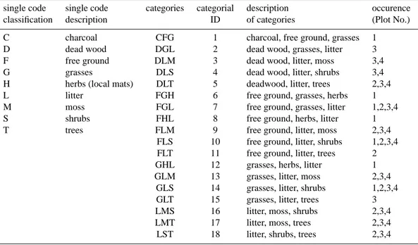
Table 1. Description for the different codes of ground cover and the combination of the 3 most abundant ground cover types for each subplot
and the finally used ground cover categories that were finally chosen. Several categories can be found in each plot, others are specific for a single plot, e.g. CFG in plot 1.
single code single code categories categorial description occurence
classification description ID of categories (Plot No.)
C charcoal CFG 1 charcoal, free ground, grasses 1
D dead wood DGL 2 dead wood, grasses, litter 3
F free ground DLM 3 dead wood, litter, moss 3,4
G grasses DLS 4 dead wood, litter, shrubs 3,4
H herbs (local mats) DLT 5 deadwood, litter, trees 2,3,4
L litter FGH 6 free ground, grasses, herbs 1
M moss FGL 7 free ground, grasses, litter 1,2,3,4
S shrubs FHL 8 free ground, herbs, litter 1
T trees FLM 9 free ground, litter, moss 2,3,4
FLS 10 free ground, litter, shrubs 1,2,3,4
FLT 11 free ground, litter, trees 2
GHL 12 grasses, herbs, litter 1
GLM 13 grasses, litter, moss 2,3,4
GLS 14 grasses, litter, shrubs 1,2,3,4
GLT 15 grasses, litter, trees 3
LMS 16 litter, moss, shrubs 2,3,4
LMT 17 litter, moss, trees 2,3,4
LST 18 litter, shrubs, trees 2,3,4
pressure fluctuations resulting from the vertical wind compo-nent, which induce a higher efflux, are transferred to the soil surface (Rayment, 2000; Janssens et al., 2000; Pumpanen et al., 2004). Each respiration chamber measurement was ac-companied by measurements, adjacent to the collar, of soil water content at 5 cm soil depth (ThetaProbe, Delta-T De-vices, Cambridge, UK) and soil temperature in the upper soil horizon at 5, 10 and 15 cm depth (LiCor 6400-09, LiCor Inc., Lincoln, NE, USA).
Foliage respiration was measured at shade and sun leaves in different heights (n=30 in 2008 andn=15 in 2009) of the dominant tree species within all inventory plots. Mea-surements were undertaken at dawn and during daytime us-ing a dark closed chamber attached to an infrared gas ana-lyzer (LI-6400, LiCor Inc., Lincoln, NE, USA). Leaf respi-ration measurements were carried out during the wet season campaigns only, since most of the leaves had already fallen off during the dry season.
As the third process (besides soil- and leaf respiration) contributing toReco, stem respiration was calculated using
plot-specific values of leaf area index (LAI). Meir and Grace (2002) found an exponential increase of aboveground woody biomass respiration with rising values of LAI for tropical ecosystems. This relation was adapted for the miombo wood-land in this study and plot and subplot specific values of LAI were used to calculate values of stem respiration instead of using a constant estimate derived from other ecosystems. This approach did not include any response of stem respira-tion to temperature as shown by Lavigne (1987). Air
temper-ature during the period under observation commonly ranged from 20–30◦C in Kataba forest.
2.4 Eddy covariance measurements and data post processing
The scaffold tower was instrumented with eddy covariance equipment, as described by Aubinet et al. (2000) and Bal-docchi et al. (2001), in September 2007. In brief, the sys-tem included a 3D sonic anemometer (Solent R3, Gill In-struments, Lymington, UK) and an infrared closed-path gas analyser (LI-7000 LiCor Inc., Lincoln, NE, USA). The EC system was accompanied with meteorological sensors (air temperature, humidity, net radiation, global radiation, pho-tosynthetic active radiation, rainfall, soil water content, etc. – Table 2). Soil water content in particular was measured in two vertical profiles (5, 10, 30, 50, 100 cm depth) using soil moisture probes (ThetaProbe, Delta-T Devices, Cambridge, UK).
Half-hourly flux averages were calculated and corrected using the Eddysoft software package (Kolle and Rebmann, 2007). This included spike detection in the raw data, trans-formation into physical values and calculation of the half hourly averages of CO2 and water vapour fluxes.
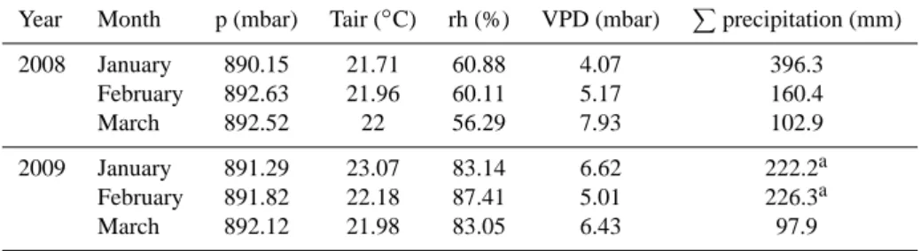
Table 2. Monthly mean of basic meteorological variables for the January – March in 2008 and 2009 measured in Kataba forest. Values for
precipitation are given as monthly sums. Measurements were undertaken at a height of 2 m.
Year Month p (mbar) Tair (◦C) rh (%) VPD (mbar) Pprecipitation (mm)
2008 January 890.15 21.71 60.88 4.07 396.3
February 892.63 21.96 60.11 5.17 160.4
March 892.52 22 56.29 7.93 102.9
2009 January 891.29 23.07 83.14 6.62 222.2a
February 891.82 22.18 87.41 5.01 226.3a
March 892.12 21.98 83.05 6.43 97.9
adue to sensor malfunction at Kataba forest, data was kindly provided by the Meteorological Dept. Mongu (distance 30 km)
vertical wind velocity (w) and temperature on the raw data according to Knohl et al. (2003) and (iv) application of sta-tionarity tests and integral turbulence characteristics as given by Foken and Wichura (1996). In addition, friction velocity (u∗) – filtering at night-time was applied (lower threshold: 0.2 m s−2, Goulden et al., 1996, Gu et al., 2005, Papale et
al., 2006). Data were also filtered for an upperu∗threshold
(0.7 m s−2)to avoid overestimation of the measured fluxes
(Merbold et al., 2009b; Gu et al., 2005), and checked for re-alistic values of atmospheric stability (z/L – Monin-Obukhov length) resulting in a “high-quality” data set.
2.5 Gap-filling and calculation of daytime ecosystem respiration
Night-time data of net ecosystem exchange that passed the quality control filtering were used to calibrate a modified ecosystem respiration (Reco)model according to Reichstein
et al. (2003, Eq. 1) using soil temperature at 5 cm depth and relative plant available water (WPar)in the first meter of the
soil as input variables.
Reco=Rref×f (Tsoil,WPAr)×g (WPAr) (1)
whereRecois the modelled respiration,Rrefis the respiration
for a site-specific temperature for biweekly periods,f andg are functions for the influence of soil temperature (Tsoil)and
relative plant available water (WPar)modified from the study
by Reichstein et al. (2003).WParwas based on measurements
of soil water content (θ )at wilting point and field capacity and used instead of relative soil water content (θr). WPar
af-fects the living tissue directly (autotrophic respiration) and the microbial biomass indirectly via the plant exudates (het-erotrophic respiration). When applyingθr instead of WPar
an overestimation ofRecocaused by a longer response of the
autotrophic component toθr seems likely but is unrealistic from the biological point of view, since plants can only ac-cess water in the soil until a certain threshold (wilting point), depending on the soil structure. Wilting point and field ca-pacity were defined by the maximum and minimum values of volumetric soil moisture measured in the very well drained
Arenosols in Kataba. WPar a was then calculated from the
measured values ofθ for 4 subsequent layers (0–0.1 m, 0.1– 0.3 m, 0.3–0.5 m and 0.5–1.0 m).
The resulting model was used to estimate daytime respi-ratory fluxes from night-time measurements. The extrapola-tion of night-time EC measurements bears the risk of high uncertainty induced by a decrease in friction velocity, result-ing from a lowerresult-ing of the boundary layer at night (Moncrieff et al., 1997; Goulden et al., 1996). Furthermore, night-time fluxes measured by EC may be biased by advection (Kutsch et al., 2008). Therefore we also used a second method to ap-proximateReco, from EC measurements, developed and
ex-plained by Lasslop et al. (2009). This method calculatesReco
from day-time data, as the intercept of the hyperbolic func-tion fitted to a plot of NEE versus global radiafunc-tion (i.e. the ecosystem scale light response curve). The approach takes account of the effects of vapour pressure deficit (VPD) in the light response and temperature regulates the response of the derived term forReco(Lasslop et al., 2009).
As a third approach to deriveReco, the online gap-filling
tool (Reichstein et al., 2005), was used. In this tool gap-filled night-time fluxes are fitted to a temperature function only (Lloyd and Taylor, 1994), ignoring the influence of soil water content, which is of crucial importance for semi-arid and arid ecosystems in Africa (Merbold et al., 2009a; Nsabi-mana et al., 2009; Archibald et al., 2009).
2.6 Stand structure, soil- and ecosystem-physiological parameters
Soil samples were collected within each subplot used for respiration measurements in 2008 and 2009 (cores 4.8 cm in diameter, 30 cm in depth). The samples were air dried in the field and shipped to a laboratory in Jena, Germany. Then, the samples were washed and sieved at 2 mm and 630 µm to separate coarse organic matter (primarily fine roots), partic-ulate organic matter (mycorrhiza and charcoal) and mineral soil associated organic matter (humic substances and black carbon). Thereafter, each subsample was dried at 40◦C, weighed and analyzed for total carbon and nitrogen content (VarioMax EL, Elemantar Analysesysteme GmbH, Hanau, Germany).
2.7 Statistical analysis
Data analysis was performed using the statistical software package SPSS 16.0 (SPSS Inc.) and Statgraphics Centurion XV (STATPOINT Technologies, Inc., Virginia, USA). Di-urnal measurements of soil CO2efflux were correlated with
soil temperature using the exponential relationship:
Rsoil=kemTsoil, (2)
whereRsoil is soil respiration (µmol m−2s−1), Tsoil is soil
temperature at 5 cm depth andkandmare coefficients. Averaged soil respiration for each categorized subplot (represented by three collars and each measured during three cycles) was fitted to soil water content with a linear function:
Rsoil=aθ+b, (3)
whereRsoilis soil respiration (µmol m−2s−1),θis soil water
content (volumetric %, 5 cm depth), a and b are constants derived from curve fitting (Table 3).
To studyRsoilspatially, mean efflux rates were normalized
for the overall average soil temperature (26◦C) and soil wa-ter content (5.5 vol. %) using a plot specific general linear model:
Rsnorm=cθ±dTsoil±hθ Tsoil±i, (4)
whereRsnormis the normalized soil CO2efflux,θ soil water
content (volumetric %),Tsoil(soil temperature a 5 cm depth
in◦C) andc,d,handiare plot specific coefficients. Statis-tics are given in Table 4. The resulting values were correlated to the above mentioned stand structural, soil- and ecosystem physiological parameters using Statgraphics Centurion XV (Statpoint Technologies Inc., Virginia, USA.). Differences in soil respiration fluxes and possible confounding meta-variables between the plots were tested using a Two-Way ANOVA of normalized values of soil respiration (Rsnorm),
where the plot-variable was used as a factor and the subplot-variable as a covariate.
2.8 Total ecosystem respiration (top-down vs. bottom-up approach)
To compare the top-down and bottom-up approaches of car-bon efflux estimation, we calculated the EC carcar-bon fluxes for half-hour periods on the days when soil respiration data were collected from chambers in the field. Only EC data which ap-plied to the specific wind sectors in the direction of each of the intensive measurement plots were used (Fig. 1).
For the bottom-up approach, comprising of soil-, leaf and stem respiration, two different calculations were done. One accounted for spatial heterogeneity of soil respiration by means of an area-weighted average, based on the categories of ground cover within the plot. Foliage respiration was scaled using the plot specific measurements of leaf respira-tion and the according values of leaf area index. Comparison was done for daytime respiration only, since there were not sufficient bottom-up data for night-time soil respiration.
3 Results
3.1 Temporal variation of soil respiration
On a diurnal time scale, soil temperature was the primary driving factor associated with variations in soil respiration during both the dry season and dry periods in the wet season resulting in an exponential increase of soil CO2 efflux with
a rise in temperature (not shown). In contrast, rain events were commonly followed by a flush of carbon dioxide to the atmosphere and an increase in respiration rates thereafter but a decrease in soil temperature for several hours after the pre-cipitation event. However, no significant relation between efflux rates and soil temperature could be shown for such cases. The magnitude of the increase varied with progress of the growing season and with the temporal pattern of precipi-tation events.
The CO2 efflux during the dry season in 2008 was
substantially less than the efflux rates measured in the wet seasons of both 2008 and 2009. Soil respiration showed a typical seasonal pattern related to soil water content (θ ), with the maximum during the rainy sea-son (subplot averages of 11.63 µmol m−2s−1 in 2008 and 12.25 µmol m−2s−1 in 2009) and the minimum during the dry season (0.94 µmol m−2s−1 in 2008). The general pat-tern of soil CO2efflux, showing an increase with rising soil
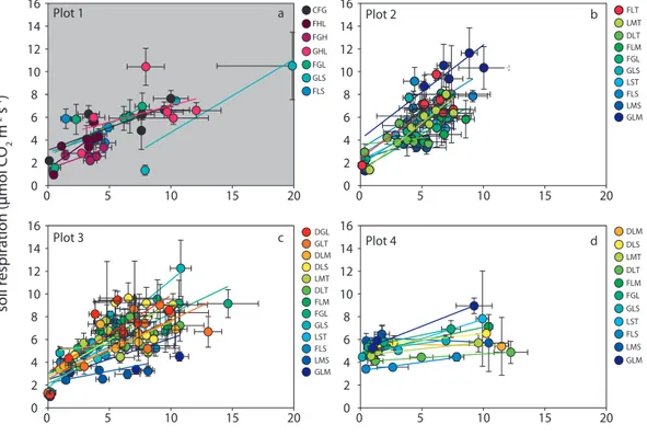
water content, was similar between and within plots. How-ever the changes were not evenly distributed within plots as illustrated by the varying slopes ofRsoilin Fig. 2.
The two interrelated factors (Tsoil, θ ) influencing Rsoil
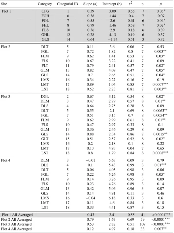
Table 3. Categories for each of the 4 plots and the statistical results of the curve fits of soil respiration (Rsoil)to soil water content (θ )within each subplot. “*” indicate significant correlations betweenRsoilandθ. Strong correlations were found for plot 4 where significance levels were not reached caused by insufficient amounts of data (2009 measurements only). Grey highlighted areas visualize the disturbed plot.
Site Category Categorial ID Slope (a) Intercept (b) r2 n p
Plot 1 CFG 1 0.39 3.09 0.55 7 0.05∗
FGH 6 0.38 1.44 0.4 7 0.07
FGL 7 0.55 2.6 0.61 6 0.04∗
FHL 8 0.79 1.46 0.58 7 0.02∗
FLS 10 0.36 2.9 0.18 6 0.39
GHL 12 0.28 4.13 0.19 6 0.37
GLS 14 0.64 −1.74 0.51 3 0.32
Plot 2 DLT 5 0.11 3.6 0.06 7 0.53
FGL 7 0.72 1.82 0.8 7 0.003∗∗
FLM 9 0.62 1.41 0.53 7 0.03∗
FLS 10 0.67 3.22 0.41 7 0.09
FLT 11 0.79 2.41 0.57 7 0.02∗
GLM 13 0.82 4.09 0.47 7 0.05∗
GLS 14 0.7 2.65 0.51 7 0.04∗
LMS 16 0.34 2.27 0.16 7 0.19
LMT 17 0.89 1.04 0.85 7 0.0007∗∗∗
LST 18 0.52 2.23 0.81 7 0.003∗∗
Plot 3 DGL 2 0.67 3.12 0.54 8 0.02∗
DLM 3 0.47 2.79 0.57 8 0.01∗∗
DLS 4 0.64 2.75 0.28 8 0.09
DLT 5 0.55 2.1 0.69 8 0.0063∗∗
FGL 7 0.51 3.15 0.7 8 0.0054∗∗
FLM 9 0.62 2.99 0.61 8 0.01∗∗
FLS 10 0.47 2.97 0.33 8 0.1
GLM 13 0.36 2.46 0.29 8 0.09
GLS 14 0.88 2.34 0.86 7 0.0015∗∗
GLT 15 0.51 2.57 0.52 8 0.02∗
LMS 16 0.2 2.18 0.1 8 0.22
LMT 17 0.13 4.93 0.04 7 0.65
LST 18 0.8 1.79 0.84 8 0.0008∗∗∗
Plot 4 DLM 3 −0.01 5.63 0.09 3 0.79
DLS 4 0.1 5.43 0.99 3 0.01∗∗∗
DLT 5 0.06 4.05 0.98 3 0.06
FGL 7 0.22 5.26 0.98 3 0.05∗
FLM 9 0.14 3.26 0.95 3 0.09
FLS 10 0.23 4.76 0.89 3 0.14
GLM 13 0.42 5.06 0.96 3 0.07
GLS 14 0.14 4.91 0.11 3 0.46
LMS 16 −0.04 6.18 0.33 3 0.6
LMT 17 0.11 4.6 0.84 3 0.18
LST 18 0.33 4.41 0.87 3 0.15
Plot 1 All Averaged 0.43 2.41 0.55 41 <0.0001∗∗∗
Plot 2 All Averaged 0.79 1.67 0.69 79 <0.0001∗∗∗
Plot 3 All Averaged 0.53 2.82 0.51 107 <0.0001∗∗∗
0 5 10 15 20 0
2 4 6 8 10 12 14 16
FLS FGH
FGL FHL
GLS CFG
GHL
Plot 1 a
soil respiration (µmol CO
2
m
-2 s -1)
Plot 3 c
0 5 10 15 20
0 2 4 6 8 10 12 14 16
GLM LMS FLS LST GLS FGL FLM DLT LMT DLS DLM GLT DGL
soil water content (5 cm depth, volumetric %)
Plot 4 d
0 5 10 15 20
0 2 4 6 8 10 12 14 16
LST DLT
FLS DLM
FLM
LMS GLS LMT DLS
FGL
GLM
Plot 2 b
0 5 10 15 20
0 2 4 6 8 10 12 14 16
GLM LMS FLS LST GLS FGL FLM DLT FLT LMT
D
isturbanc
e gr
adien
t
Fig. 2. Relation ofRsoil, measured during the field campaigns 2008 and 2009, plotted against soil water content (θ )at a depth of 5 cm along
the disturbance gradient for each subplot (coloured) and plot. Similar categories are represented by the same color. Detailed information on categorized subplots and statistics are given in Tables 1 and 2.
Table 4. Statistics and coefficients of the general linear model,
in-cluding soil temperature and soil water content as primary factors influencing soil respiration on temporal time scales are given. n gives the amount of data available for each plot,pthe significance level andc,d,handithe plot specific coefficients. Grey highlighted is the disturbed plot.
Plot n r2 p c d h i
1 173 0.34 0.000∗∗∗ −0.43 −0.21 0.03 8.91
2 213 0.53 0.000∗∗∗ −0.36 −0.19 0.04 7.54
3 325 0.47 0.000∗∗∗ −0.28 −0.0006 0.03 2.85
4 108 0.09a 0.01∗∗ 0.24 0.19 −0.005 0.33
asmall values of the correlation coefficient, originate from 50% less
replicates collected in plot 4.
Average wet season efflux was slightly higher in 2009 compared to 2008 for the disturbed plots (Fig. 4a) and lower for the undisturbed site (Fig. 4b) – not shown for plots 3 and 4, showing a similar picture as Fig. 4b.
Table 5. Descriptive and ANOVA statistics are shown for soil
res-piration values along the disturbance gradient. The grey highlighted lines show the disturbed plot where the non-highlighted values rep-resent the undisturbed plots. Differences in average plot respiration were significant in the wet season 2008. Plot 4 was observed in 2009 only.
average
Year/ Plot Rsnorm standard coefficient (%) ANOVA
Season (µmol m−2s−1) deviation of variation p-Value
2008/Wet 1 4.94 1.31 26.51
2 6.54 2.00 30.59
3 6.53 1.85 28.38
4 n.a. n.a. n.a.
0.000∗∗∗
2008/Dry 1 2.93 1.26 42.96
2 5.64 2.02 35.87
3 2.46 0.38 15.65
4 n.a. n.a. n.a.
0.000∗∗∗
2009/Wet 1 5.80 2.54 43.88
2 6.00 1.69 28.20
3 5.59 1.43 25.66
4 6.01 1.43 23.87
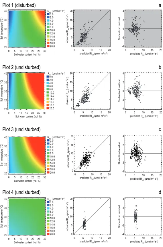
Plot
3
(undisturbed)
c
Plot
1
(disturbed)
a
Plot
4
(undisturbed)
d
Plot
2
(undisturbed)
b
0 5 10 15 20 25 30
Soil water content (vol. %) 20
25 30 35 40
Soil temperature (°C)
Rsoil (µmol m-2 s-1) 0.0 2.0 4.0 6.0 8.0 10.0 12.0 14.0 16.0 18.0 20.0
0 5 10 15 20
predicted Rsoil (µmol m
-2 s-1)
0 5 10 15 20 o b se rv e d Rsoil (µmol m
-2 s
-1)
0 5 10 15 20
predicted Rsoil (µmol m
-2 s-1)
-4 -2 0 2 4 S tu d e n tiz e d r e si d u a l
0 5 10 15 20 25 30
Soil water content (vol. %) 20
25 30 35 40
Soil temperature (°C)
Rsoil (µmol m
-2 s-1)
0.0 2.0 4.0 6.0 8.0 10.0 12.0 14.0 16.0 18.0 20.0
0 5 10 15 20
predicted Rsoil (µmol m
-2 s-1)
0 5 10 15 20 o b se rv e d Rsoil (µmol m
-2 s
-1)
0 5 10 15 20
predicted Rsoil (µmol m-2 s-1) -4 -2 0 2 4 S tu d e n tiz e d r e si d u a l
0 5 10 15 20 25 30
Soil water content (vol. %) 20 25 30 35 40 S o
il temperature (°C)
Rsoil (µmol m-2 s-1) 0.0 2.0 4.0 6.0 8.0 10.0 12.0 14.0 16.0 18.0 20.0
0 5 10 15 20
predicted Rsoil (µmol m
-2 s-1)
0 5 10 15 20 o b se rv e d R soil (µmol m
-2 s
-1)
0 5 10 15 20
predicted Rsoil (µmol m
-2 s-1)
-4 -2 0 2 4 S tu d e n tiz e d r e si d u a l
Fig. 3. General linear models explaining soil respiration using soil temperature and soil water content as predictors. Panels a–d represent
Category (classes of ground cover)
Rsoil
(µmol m
-2 s
-1)
Plot 2 - undisturbed
GLM
LMSFLSLSTGLSFGLFLMDLTFLTLMT
0 2 4 6 8 10 12 14 16
Plot 1 - disturbed
FLS
GLSFGLGHLFGHFHLCFG
black = 2008 wet white = 2008 dry grey = 2009 wet
a b
Fig. 4. Differences in averaged soil respiration are shown for
sub-plots for the different years and seasons. Data for only 2 of the in-ventory plots are given, where (a) (grey highlighted) represents the disturbed area showing higher values ofRsoilin 2009 (grey bars) compared to 2008 (black bars) and (b) represents the undisturbed area showing the exactly opposite result. Smallest efflux rates were always observed during the dry season (white bars). Categories are given according to Tables 1 and 2.
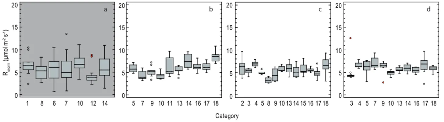
3.2 Small scale spatial variation of soil respiration (within plots)
Spatial variation of respiration was based a priori on the classes of ground cover (categories). This assumption was tested for each plot separately using One-Way ANOVAs. Soil respiration varied significantly between subplots in all of the 4 plots (Fig. 5).
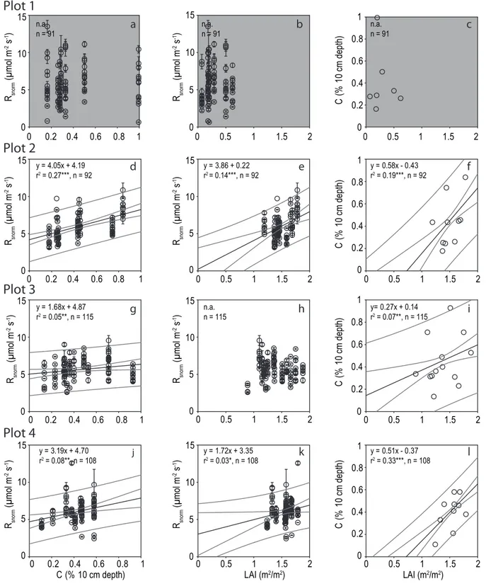
Leaf area index, soil carbon content and belowground biomass are variables changing at a lower frequency in time when compared to meteorological variables. These variables were chosen to analyse the spatial variations of normalised soil respiration rates (Rsnorm- normalized for temperature and
water content). The only parameter identified in this study explaining significant portions of the spatial variability of Rsnorm within the undisturbed plots was soil carbon content
(vol. %) at 10 cm depth (Fig. 6d, g and j). Soil carbon content explained up to 27% of the spatial variation ofRsnorm. Leaf
area index was found to be a predictor of soil respiration in only 2 of the 4 inventory plots (Fig. 6e and k) but not for the other 2 plots (Fig. 6b and h). None of the before mentioned variables explained the variations of soil respiration in the disturbed plot (Fig. 6a, b and c).
Carbon content in the soil is commonly related to above-and belowground biomass above-and litter inputs in an ecosystem (Jenkinson et al., 1992, 1999). Therefore we plotted below-ground carbon content (%, 10 cm depth) against leaf area in-dex, an indirect measure of biomass and the associated lit-ter (and carbon) inputs. Our results show a positive rela-tion between belowground carbon content and leaf area index (Fig. 6f, i and l) for the undisturbed plots.
3.3 Spatial variation of soil respiration along the disturbance gradient (between plots)
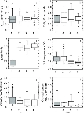
There was no significant difference in respired carbon be-tween the disturbed and undisturbed plots (Table 5) in 2009 when measurements were available for all plots. Similarly, no defined trend in soil respiration was observed along the disturbance gradient during the dry season 2008 (Table 5). Soil respiration in plot 2 clearly exceeded values measured in Plot 1 and 3. In contrast, during the wet season 2008, car-bon fluxes varied along the disturbance gradient (data from Plot 4 was not available at this time – Table 5). Coefficients of variation were always highest in the disturbed area and de-clined towards the most undisturbed plot for all wet season measurements (Table 5).
The variation in respiratory fluxes in 2009 was poorly ex-plained by carbon content at a depth of 10 cm (Fig. 7a and b), showing no clear distinction between the disturbed and the undisturbed areas. No relation could be established be-tween the large and significant differences in leaf area index between the disturbed and undisturbed sites (Fig. 7c) to the soil CO2 efflux rates in the wet season 2009 (Table 5 and
Fig. 7c).
Soil temperature was lower in the undisturbed plots than in the disturbed plot (Fig. 7d). Differences in soil carbon content (10 cm depth – Fig. 7b), soil water content (vol.% – Fig. 7e) and charcoal content (mg, 10 cm depth – Fig. 7f) between plots were not significant.
3.4 Total daytime carbon loss
Total carbon emitted by respiration from the ecosystem to the atmosphere was highest in the wet season 2008/2009 (high values in Fig. 8) and lowest during the dry season 2008 (low values in Fig. 8). The two different bottom-up approaches differed only slightly from each other. The approach ac-counting for spatial heterogeneity inRsoilresulted in slightly
less deviation from the 1:1 line (Fig. 8b) compared to simple averaging ofRsoil (Fig. 8a). However, the variation of the
top-down as well as for the bottom-up approaches was high. Assuming the chamber-based bottom-up approach provides more realistic values of the real carbon loss from ecosys-tems, none of the 3 different methods for EC-based estima-tion matched the values from the process approach perfectly (Fig. 8a and b), but all were within the standard deviation of the process up-scaling. During the dry season in 2008 the top-down approaches underestimated the carbon loss relative to the bottom-up calculations across all plots (Fig. 8a and b). Two different top-down approaches based on night-time data, resulted (black and white dots) in a maximum deviation of 20% from the bottom-up derived values. The top-down approach using daytime fluxes, as described by Lasslop et al. (2009), underestimatedRecoby up to 25% for the different
8 6 7 10 12 14 1
0 5 10 15 20
Rsnorm
(µmol m
-2 s -1)
Category 0
5 10 15 20
13 16
10 14 18
7 9
5 11 17
0 5 10 15 20
18
5 10
3 4 7 9 13141617 0
5 10 15 20
13 16
10 14 18
8 9
5 17
4
3 15
2
a b c d
Fig. 5. Differences in subplot efflux rates in 2009 shown for each inventory plot (a–d representing plot 1–4). Average efflux rates deviated
strongly between subplots. On the contrary, efflux rates of different subplots between plots showed similar values and vice versa. Variation in subplot specific efflux rates was highest in the disturbed plot 1 (a). Categories are given according to Tables 1 and 2.
On the other hand the night-time based model including a response to soil water content and temperature overestimated fluxes in the wet seasons (black dots). Generally, each model had its strengths, either for the disturbed or undisturbed plots in the dry and the wet season (not shown). Similarly each top-down approach had its weaknesses. The best correlations were given by the methods using night-time data of Reco
(white dots –r2=0.9/0.81 and black dots –r2=0.88/0.92).
4 Discussion
Portable soil chambers are well-suited to investigate spatial differences in soil CO2efflux, but do not allow permanent
long-term observations (Soe and Buchmann, 2005). In con-trast, static automatic chambers (Irvine and Law, 2002) and the understory EC method (Baldocchi and Meyers, 1991) provide continuous measurements but are often not applica-ble due to their complexity and expense (Pumpanen et al., 2004). In our study, the two chamber types were combined during three measuring campaigns.
We measured diurnal time-courses of soil respiration with an automatic open chamber and showed that during a day without rain, the temporal variation of soil respiration fol-lowed soil temperature. This exponential function of soil temperature has already been shown by several other stud-ies (Evrendilek et al., 2005; Zimmermann et al., 2009). Sud-den peaks in soil CO2efflux immediately after rainfall events
confirm previous findings by Inglima et al. (2009) and Lee et al. (2004). Up to date it remains a major challenge to quan-tify and to model these pulses. The peaks in soil CO2
ef-flux commonly result from 2 different processes: (1) during the rain event a “solid” water layer penetrates the ground, pushing CO2 from the pore spaces in the soil towards the
atmosphere, explaining the sudden peak (Lee et al., 2004). The strong decrease in efflux rates after the burst of CO2can
also be explained CO2storage in the soil. Soil pores are
“de-pleted” in CO2and need some time to refill. (2) Higher
emis-sions of CO2after a rainfall event were explained by priming
effects of the water inputs on microbial activity and decom-position processes in the soil (Unger et al., 2010, Borken and Matzner, 2009).
At seasonal timescales, soil water content became the primary controlling factor. Observations similar to our re-sults were shown by Epron et al. (2004) and Nouvellon et al. (2008) in an Eucalyptus plantation in Congo, which re-ceives slightly more rain per year than Kataba, but also ex-periences a strong distinction between the wet and dry sea-son. Studies in a semiarid ecosystem in the Mediterranean by Evrendilek et al. (2005) and Maestre and Cortina (2003) also showed a seasonal dependency ofRsoilon soil water content.
Accounting for the spatial variability ofRsoilis more
dif-ficult than accounting for temporal variations (Rayment and Jarvis, 2000; Baldocchi et al., 2006). Often, spatial varia-tion ofRsoilcannot be explained by microclimatic variables
such as soil moisture and temperature, whilst it can be ex-plained by the variation in biological activity and soil chem-istry (Law et al., 2001; Xu and Qi, 2001). For this purpose, Rsoilis often normalized to a standard soil temperature,
stan-dard soil moisture or both. In this study we corrected for both parameters to the overall averages measured during the cam-paigns, 26◦C of soil temperature and 5.5 vol. % of soil water,
respectively. Several studies have found strong correlations betweenRsoiland biological factors such as the thickness of
the moss layer (Rayment and Jarvis, 2000), root density or distance to the nearest tree (Soe and Buchmann, 2005; Tang and Baldocchi, 2005).
At Kataba forest, spatial heterogeneity of soil respiration (Rsnorm)was explained by soil carbon content (10 cm depth)
in the undisturbed plots only. Explaining this within-plot cor-relation betweenRsnormand belowground carbon we
Plot 3
y = 3.86 + 0.22
r2 = 0.14***, n = 92
0 0.5 1 1.5 2 0
5 10 15
Rsnorm
(µmol m
-2 s -1) y = 4.05x + 4.19
r2 = 0.27***, n = 92
0 0.2 0.4 0.6 0.8 1 0
5 10 15
Rsnorm
(µmol m
-2 s -1)
y = 0.58x - 0.43
r2 = 0.19***, n = 92
0 0.5 1 1.5 2 0
0.2 0.4 0.6 0.8 1
C
(%
1
0 cm depth)
Plot 4
Plot 1
Plot 2
y = 3.19x + 4.70
r2 = 0.08**, n = 108
0 0.2 0.4 0.6 0.8 1 C (% 10 cm depth) 0
5 10 15
Rsnorm
(µmol m
-2 s -1)
y = 0.51x - 0.37
r2 = 0.33***, n = 108
0 0.5 1 1.5 2 LAI (m2/m2)
0 0.2 0.4 0.6 0.8 1
C
(%
1
0 cm depth)
y = 1.72x + 3.35
r2 = 0.03*, n = 108
0 0.5 1 1.5 2 LAI (m2/m2) 0
5 10 15
Rsnorm
(µmol m
-2 s -1)
0 0.5 1 1.5 2 0
5 10 15
Rsnorm
(µmol m
-2 s -1)
0 0.2 0.4 0.6 0.8 1 0
5 10 15
Rsnorm
(µmol m
-2 s -1)
0 0.5 1 1.5 2 0
0.2 0.4 0.6 0.8 1
C
(%
1
0 cm depth)
c
d
e
f
g
h
i
j
k
l
y = 1.68x + 4.87
r2 = 0.05**, n = 115
0 0.2 0.4 0.6 0.8 1 0
5 10 15
Rsnorm
(µmol m
-2 s -1)
0 0.5 1 1.5 2 0
5 10 15
Rsnorm
(µmol m
-2 s -1)
y= 0.27x + 0.14
r2 = 0.07**, n = 115
0 0.5 1 1.5 2 0
0.2 0.4 0.6 0.8 1
C
(%
1
0 cm depth)
n.a. n = 91
n.a. n = 115
b
n.a. n = 91
a
n.a. n = 91
Fig. 6. The figure shows the relations between normalized soil respiration (Rsnorm)and soil carbon content (10 cm depth) and leaf area index
1 2 3 4 0
0.2 0.4 0.6 0.8 1
C
(%
, 10 cm depth)
1 2 3 4
0 3 6 9 12 15
Rsnorm
(µmol m
-2 s -1)
1 2 3 4
0 0.5 1 1.5 2
LAI (m
2/m 2)
1 2 3 4
20 25 30 35 40
Soil temperature (°C)
1 2 3 4
0 5 10 15 20 25 30
Soil water content (vol. %)
Plot
1 2 3 4
0 0.5
1 1.5
2
Charcoal content (mg, 10 cm depth)
Plot
a b
c d
e f
Fig. 7. Plot specific values for normalized soil respiration (a) and
several biotic (b and c) and abiotic parameters (d, e and f) are shown to visualize between plot differences – 2009 only. Average values of the various variables in Plot 1 (disturbed) did not deviate sig-nificantly from values derived for the three other plots (2–4, undis-turbed). The only exception was shown for values of leaf area index. Filled dots represent outliers.
baumiana and Xylopia odoratissima shrubs that seem to cre-ate micro-zones of decreased turbulence near the forest floor. Hence, the appearing higher litter deposition at these micro-sites will increase abundance and turnover of belowground biomass and attract roots and mycorrhiza (King et al., 2001). Leaf area index, an indirect measure for biomass (Churkina et al., 2003) and therefore also associated with carbon con-tent (Fig. 6) was only a poor predictor for the spatial variation of soil respiratory efflux. Referring to the above mentioned hot spots of soil carbon we assume an underestimation of the presented LAI values at these hot spots, caused by the method applied. Leaf area index was calculated from hemi-spheric photographs which were taken at a height of 1 m and therefore mostly above the grass/herb layer.
None of the before mentioned variables explained the within-plot variation ofRsnormin the disturbed plot. Neither
did other biotic and abiotic parameters such as belowground biomass or charcoal content as proposed by several studies
(e.g. Salimon et al., 2004; Maestre and Cortina, 2003). The highly variable flux estimates and heterogeneity observed in the disturbed area may be explained by the disturbance itself. First of all, regular disturbance such as tree logging was still occurring at the site, resulting in changes in the aboveground biomass and accordingly in less organic compounds being transported from the leaves to the root system (Kuzyakov and Gavrichkova, 2010). This again leads to lower rates of root respiration contributing largely to total soil respiration (Kuzyakov and Gavrichkova, 2010). Regular cattle grazing may also have contributed to spatial variations in soil respi-ration fluxes. In addition, remnants of charcoal kilns besides very grassy patches (occurring after clearing) and deserted patches resulted in a large heterogeneity aboveground as well as belowground without showing clear trends in respiration rates. Prove for the varying variables driving spatial hetero-geneity of carbon emissions from the soil in Kataba forest, can only be given when conducting further and more detailed measurements.
Along the gradient from plot one in the North to plot four in the South of the study area (Fig. 1) respiratory carbon fluxes from the soil did not show a significant trend in 2009 as hypothesized, neither did soil carbon content. The large magnitude of efflux rates in plot 2 compared to plots 1 and 3 during the dry season 2008 could only be explained by the differences in vegetation structure. Plot 2 was characterized by trees, larger in height and diameter at breast height when compared to the other plots (1 and 3). According to Holdo (2009) Brachystegia spiciformis trees root deeper than other miombo species and therefore have access to deeper water layers, resulting in larger CO2efflux from the soil (root
res-piration).
Decreases in soil temperatures were found towards the undisturbed plots, whereas values for soil water content and charcoal content did not vary significantly. The only vari-able showing a strong distinction between the disturbed and undisturbed areas was leaf area index. Once again we explain an underestimation of LAI with the method applied to de-rive estimates, particularly in the disturbed plot, where only parts of the grass layer were included. Our estimates of LAI primarily accounted for tree and shrub LAI, and only few grasses (larger than 1 m) were included resulting in a possi-ble explanation for not having found a correlation between CO2efflux rates and LAI along the disturbance gradient.
RecoRsoil/Rstem/Rleaf (g C m-2 12hr-1)
all averaged
0 1 2 3 4 5
Reco
Eddy
(g C m
-2 12hr -1)
0 1 2 3 4 5
RecoEddy (WPAr/Tsoil model) RecoEddy (Lasslop et al.)
RecoEddy (Reichstein et al. )
a
1RecoRsoil/Rstem/Rleaf (g C m-2 12hr-1)
including spatial heterogeneity
0 1 2 3 4 5
Reco
Eddy
(g C m
-2 12hr -1)
0 1 2 3 4 5
RecoEddy (WPAr/Tsoil model) RecoEddy (Lasslop et al.)
RecoEddy (Reichstein et al. )
b
1Fig. 8. Total carbon loss (g C m−2)during 12 daytime hours (6 a.m.–6 p.m.) for each plot during the different seasons (wet season =
high values, dry season = smaller values). Three different approaches were used to calculate daytime ecosystem respiration from eddy covariance data: (1) (black dots, black solid regression) a model, including the response ofRecoto relative plant available water (0–100 m) and soil temperature (5 cm depth) parameterized biweekly from high quality nocturnal data; (2) (grey dots, grey solid regression) a model recently developed by Lasslop et al. (2009); (3) (white dots, black dotted regression) were values ofRecoreceived from a gapfilling – and fluxpartitioning tool (Reichstein et al., 2003). Two different methods were used for the bottom-up approach (a) averaging all measurements of soil- and leaf respiration plus the calculated values of stem respiration and (b) accounting for spatial heterogeneity by the categorized soil CO2efflux plus leaf- and stem respiration. All bars are given +/- SD. The red line shows the 1:1 line, the grey highlighted area show the 20% deviation from the 1:1 line. (a) white:r2=0.90,p <0.0001,n=9, y0= −0.12, a = 0.97 grey:r2=0.7,p=0.001,n=9, y0=0.51, a = 1.03 black: r2=0.81,p=0.0002, n=9, y0=0.09, a = 1.09 (b) white: r2=0.88,p <0.0001, n=9, y0= −0.27, a = 1.03 grey: r2=0.84,p=0.0001,n=9, y0= −0.97, a = 1.2 black:r2=0.92,p <0.0001,n=9, y0= −0.3, a = 1.24
by regeneration did not affect soil carbon very much as also shown by Chidumayo and Kwibisa (2003) and Chidumayo (1991).
High values of soil water content along the gradient were explained by several measurements being taken on remnant charcoal kilns. The specific structure of charcoal is known for its high water holding capacity (DeLuca and Aplet, 2008) and therefore resulted in high amounts of soil water.
Generally, values for carbon concentrations found in the top soils in our study (0.69%–3.33%) are in the same order of magnitude as those found by Walker and Desanker (2004) for comparable miombo woodlands in Malawi (1.2%–3.7%). Differences in belowground carbon concentrations between intact and disturbed sites reported by Walker and Desanker (2004) could not be shown for Kataba forest.
The expected decrease in charcoal content towards the undisturbed sites could not be shown, even though differ-ent amounts (not significant) of charcoal were found in the four plots. The observed charcoal concentration in the undis-turbed area may be a result of the history of the site. Low intensity ground fires are common for miombo woodlands and important to sustain the forest structure (Kikula, 1986) resulting in the occurrence of charcoal in all plots.
The results of the soil respiration study were compared to EC measurements since the simultaneous application of sev-eral methods is a more robust way to estimate the carbon dynamics of an ecosystem (Knohl et al., 2008; Wang et al., 2010). Continuous flux measurements using the eddy co-variance technique (Baldocchi and Meyers, 1998; Aubinet et al., 2000) have become one of the widely accepted tools amongst others e.g. biomass inventories (Mund et al., 2002), atmospheric inversions (House et al., 2003) and up-scaling of process measurements (Nouvellon et al., 2008; Kutsch et al., 2001) to study ecosystem carbon budgets.
In this study we evaluated respired carbon only. For our comparison between the bottom-up and top-down methods, we calculatedRecoby summing-up soil respiration, stem
Chamber measurements were conducted during daytime hours. Therefore we had to calculate daytime respiration from EC. For this purpose we used the same methods that are usually applied for the partitioning of EC fluxes intoReco
and gross photosynthesis (Reichstein et al., 2005; Papale et al., 2006; Lasslop et al., 2009), which are based on the tem-perature response curve of night-time respiration or the light response curve of NEE. Their drawback is that night-time EC measurements are often highly uncertain (Aubinet, 2008; Goulden et al., 1996; Moncrieff et al., 1997; Van Gorsel et al., 2007). However, since the topography of the area is very flat and due to the thorough quality filtering criteria we used prior to our data analysis, we assume that the night-time data we used are reliable.
Reco values obtained from EC flux partitioning were
within the standard deviation of the up-scaled process mea-surements during the two wet seasons. We found the best matching between the top-down approach following the two different Reichstein et al. (2003, 2005) models and the bottom-up approaches (Fig. 8b). The model including soil moisture and temperature as a driving variables (Reich-stein et al., 2003) performed better when compared to the bottom-up approach that accounted for spatial heterogeneity (Fig. 8b). Whereas the model, using temperature as a single driving factor (Reichstein et al., 2005), performed as good when spatial variability was not considered in the bottom-up values (Fig. 8a). The Lasslop et al. (2009) approach over-and underestimated up-scaledRecostronger. Differences
be-tween the bottom-up approach, which included soil hetero-geneity and the Lasslop et al. (2009) as well as the Reich-stein et al. (2005) model, can be explained by soil tempera-ture used as the only modifier. We conclude that the strong influence of soil water content needs to be considered in arid and semi-arid ecosystems (Epron et al., 2004) as done in method 1. Remaining differences between the top-down and the bottom-up values may be explained by biweekly parame-terization of the model, and the short term complexity ofRsoil
to rain pulses, as recently shown by Williams et al. (2009) for a savanna in South Africa, as well as by uncertainties in the up-scaling procedure of the bottom-up model.
5 Conclusions
Besides already known variables, such as temperature and stand structure, influencing the temporal and spatial varia-tion of soil respiravaria-tion we could identify the importance of soil properties and defined moisture inputs as additional im-portant driving factors of soil respiration in miombo wood-lands.
When comparing plots of different degrees of disturbance, spatial heterogeneity of soil respiration was found to depend on soil properties such as carbon content. At high distur-bance levels, plot-internal heterogeneity inRsoildepended on
the disturbance itself, particularly on position and impact of charcoal kilns. To the contrary, lower disturbance resulted in a different pattern, with soil organic carbon content being the main driver. We assume that disturbance at high levels, leads to increasing heterogeneity aboveground and therefore accordingly to large variations in soil respiration. In the dens-est plot (4) with lowdens-est disturbance spatial heterogeneity of soil respiration and aboveground structures was small.
Up-scaled values that accounted for spatial heterogeneity resulted in slightly but not significantly lower values for av-erage plot efflux. The comparisons between top-down de-rived values forReco(EC technique) were within the range
of bottom-up derived values (chamber up-scaling). Nonethe-less, a considerable under- and overestimation was found in flux partitioning methods that used over-simple temperature models to extrapolate night-time fluxes to daytime, or using the daytime light response curve to estimate respiration. We suggest that both top-down methods and bottom-up methods should be applied in order to improve confidence in the re-sults.
Appendix A
Abbreviations
CO2 carbon dioxide
LAI leaf area index
Reco total ecosystem respiration
EC eddy covariance NEE net ecosystem exchange GPP gross primary production WPAr relative plant available water θ soil water content
θr relative soil water content VPD water vapour pressure deficit ANOVA analysis of variance
Rsoil soil respiration
Rleaf leaf respiration
Rstem stem respiration
Rsnorm normalized soil respiration
Tsoil soil temperature
Acknowledgements. This study was funded as part of the CarboAfrica Initiative (EU, Contract No: 037132). We thank Manyando and Lumbala, the incredible strong helping hands in the field, the Max-Planck Institute for Biogeochemistry, in particular the field experiments group, Olaf Kolle, Martin Hertel, Kerstin Hippler and Karl K¨ubler for help during the setup and regular maintenance, technical knowledge and additional instruments installed at the site in Mongu, Zambia. E.-D. Schulze for providing additional institutional funding. We are thankful to Corinna Rebmann for assistance during EC data processing and comments while preparing the manuscript as well as Gitta Lasslop for running the data through a different algorithm to flux partition EC data. Comments of 3 anonymous reviewers helped severely to improve an earlier version of the manuscript.
The service charges for this open access publication have been covered by the Max Planck Society.
Edited by: A. Arneth
References
Archibald, S., Roy, D. P., van Wilgen, B. W., and Scholes, R. J.: What limits fire? An examination of drivers of burnt area in Southern Africa, Glob. Change Biol., 15, 613–630, 2009. Aubinet, M., Grelle, A., Ibrom, A., Rannik, ¨U., Moncrieff, J.,
Fo-ken, T., Kowalski, A., Martin, P., Berbigier, P., Bernhofer, C., Clement, R., Elbers, J., Granier, A., Gr¨unwald, T., Morgenstern, K., Pilegaard, K., Rebmann, C., Snijders, W., Valentini, R., and Vesala, T.: Estimates of the annual net carbon and water ex-change of forests: the EUROFLUX methodology, Adv. Ecol. Res., 30, 113–175, 2000.
Aubinet, M., Heinesch, B., Perrin, D., and Moureaux, C.: Dis-criminating net ecosystem exchange between different vegeta-tion plots in a heterogeneous forest, Agr. Forest Meteorol., 132, 315–328, 2005.
Aubinet, M.: Eddy covariance CO2flux measurements in nocturnal conditions: An analysis of the problem, Ecol. Appl., 18, 1368– 1378, 2008.
Bahn, M., Kutsch, W. L., Heinemeyer, A.: Synthesis: emerging issues and challenges for an integrated understanding of soil car-bon fluxes, in: Soil Carcar-bon Dynamics – An Integrated Method-ology, edited by: Kutsch, W. L., Bahn, M., and Heinemeyer, A., Cambridge University Press, 257–271, 2009.
Baldocchi, D. D. and Meyers, T. P.: Trace Gas-Exchange above the Floor of a Deciduous Forest .1. Evaporation and Co2 Efflux, J. Geophys. Res.-Atmos., 96, 7271–7285, 1991.
Baldocchi, D. D. and Meyers, T.: On using eco-physiological, mi-crometeorological and biogeochemical theory to evaluate carbon dioxide, water vapor and trace gas fluxes over vegetation: a per-spective, Agr. Forest Meteorol., 90, 1–25, 1998.
Baldocchi, D. D., Falge, E., Gu, L. H., Olson, R., Hollinger, D., Running, S., Anthoni, P., Bernhofer, C., Davis, K., Evans, R., Fuentes, J., Goldstein, A., Katul, G., Law, B., Lee, X. H., Malhi, Y., Meyers, T., Munger, W., Oechel, W., U, K. T. P., Pilegaard, K., Schmid, H. P., Valentini, R., Verma, S., Vesala, T., Wilson, K., and Wofsy, S.: FLUXNET: A new tool to study the temporal and spatial variability of ecosystem-scale carbon dioxide, water
vapor, and energy flux densities, Bull. Amer. Meteorol. Soc., 82, 2415–2434, 2001.
Baldocchi, D. D., Tang, J., and Xu, L.: How switches and lags in biophysical regulators affect spatial-temporal variation of soil respiration in an oak-grass savanna, J. Geophys. Res., 111, G02008, doi:10.1029/2005JG000063, 2006.
Bond-Lamberty, B. and Thomson, A.: Temperature-associated in-creases in the global soil respiration record, Nature, 464, 579– 582, 2010.
Borken, W. and Matzner, E.: Reappraisal of drying and wetting ef-fects on C and N mineralization and fluxes in soils, Glob. Change Biol. 15, 808–824, 2009.
Borken, W., Xu, Y. J., Davidson, E. A., and Beese, A.: Site and temporal variation of soil respiration in European beech, Nor-way spruce, and Scots pine forests, Glob. Change Biol., 8, 1205– 1216, 2002.
Buchmann, N.: Biotic and abiotic factors controlling soil respira-tion rates in Picea abies stands, Soil Biol. Biochem., 32, 1625– 1635, 2000.
Chidumayo, E. N.: Woody Biomass Structure and Utilization for Charcoal Production in a Zambian Miombo Woodland, Biore-source Technol., 37, 43–52, 1991.
Chidumayo, E. N. and Kwibisa, L.: Effects of deforestation on grass biomass and soil nutrient status in miombo woodland, Zambia, Agr. Ecosyst. Environ., 96, 97–105, 2003.
Churkina, G., Tenhunen, J., Thornton, P., Falge, E. M., Elbers, J. A., Erhard, M., Grunwald, T., Kowalski, A. S., Rannik, U., and Sprinz, D.: Analyzing the ecosystem carbon dynamics of four European coniferous forests using a biogeochemistry model, Ecosystems, 6, 168–184, 2003.
Davidson, E. A., Belk, E., and Boone, R. D.: Soil water content and temperature as independent or confounded factors control-ling soil respiration in a temperate mixed hardwood forest, Glob. Change Biol., 4, 217–227, 1998.
DeLuca, T. H. and Aplet, G. H.: Charcoal and carbon storage in forest soils of the Rocky Mountain West, Front. Ecol. Environ., 6, 18–24, 2008.
Epron, D., Nouvellon, Y., Roupsard, O., Mouvondy, W., Mabiala, A., Saint-Andre, L., Joffre, R., Jourdan, C., Bonnefond, J. M., Berbigier, P., and Hamel, O.: Spatial and temporal variations of soil respiration in a Eucalyptus plantation in Congo, Forest Ecol. Manage., 202, 149–160, 2004.
Evrendilek, F., Ben-Asher, J., Aydin, M., and Celik, I.: Spatial and temporal variations in diurnal CO2fluxes of different Mediter-ranean ecosystems in Turkey, J. Environ. Monitor., 7, 151–157, 2005.
Foken, T. and Wichura, B.: Tools for quality assessment of surface-based flux measurements, Agr. Forest Meteorol., 78, 83–105, 1996.
Goulden, M. L., Munger, J. W., Fan, S.-M., Daube, B. C., and Wofsy, S. C.: Measurements of carbon sequestration by long-term eddy covariance: methodsand critical evaluation of ac-curacy, Glob. Change Biol., 2, 169–182, doi:10.1111/j.1365-2486.1996.tb00070.x, 1996.
Grace, J., San Jose, J., Meir, P., Miranda, H. S., and Montes, R. A.: Productivity and carbon fluxes of tropical savannas, J. Biogeogr., 33, 387–400, 2006.
and Xu, L. K.: Objective threshold determination for nighttime eddy flux filtering, Agr. Forest Meteorol., 128, 179–197, 2005. Hanson, P. J., O’Neill, E. G., and Chambers, M. L. S.: Soil
respi-ration and litter decomposition, in: North American Temperate Deciduous Forest Responses to Changing Precipitation Regimes, edited by: Hanson, P. J. and Wullschleger, S. D., Springer, New York, 163–189, 2003.
House, J. I., Prentice, I. C., Ramankutty, N., Houghton, R. A., and Heimann, M.: Reconciling apparent inconsistencies in es-timates of terrestrial CO2sources and sinks, Tellus B, 55, 345– 363, 2003.
Inglima, I., Alberti, G., Bertolini, T., Vaccari, F. P., Gioli, B., Miglietta, F., Cotrufo, M. F., and Peressotti, A.: Precipitation pulses enhance respiration of Mediterranean ecosystems: the bal-ance between organic and inorganic components of increased soil CO2efflux, Glob. Change Biol., 15, 1289–1301, 2010.
Irvine, J. and Law, B. E.: Contrasting soil respiration in young and old-growth ponderosa pine forests, Glob. Change Biol., 8, 1183– 1194, 2002.
Janssens, I. A., Kowalski, A. S., Longdoz, B., and Ceulemans, R.: Assessing forest soil CO2efflux: an in situ comparison of four technques, Tree Physiol., 20, 23–32, 2000.
Jenkinson, D. S., Harkness, D. D., Vance, E. D., Adams, D. E., and Harrison, A. F.: Calculating net primary production and annual input of organic-matter to soil from the amount and radiocarbon content of soil organic matter, Soil Biol. Biochem. 24, 295–308, 1992.
Jenkinson, D. S., Meredith, J., Kinyamario, J. I., Warren, G. P., Wong, M. T. F., Harkness, D. D., Bol, R., and Coleman, K.: Estimating net primary production from measurements made on soil organic-matter, Ecology, 80, 2762–2773, 1999.
Kanschik, W. and Becker, B.: Dry miombo: Ecology of its major plant species and their potential use as bio-indicators, Plant Ecol., 155, 139–146, 2001.
Kikula, I. S.: The Influence of Fire on the Composition of Miombo Woodland of Southwest Tanzania, Oikos, 46, 317–324, 1986. King, J. S., Pregitzer, K. S., Zak, D. R., Sober, J., Isebrands, J. G.,
Dickson, R. E., Hendrey, G. R., and Karnosky, D. F.: Fine-root biomass and fluxes of soil carbon in young stands of paper birch and trembling aspen as affected by elevated atmospheric CO2 and tropospheric O3, Oecologia, 128, 237–250, 2001.
Knohl, A., Schulze, E. D., Kolle, O., and Buchmann, N.: Large carbon uptake by an unmanaged 250-year-old deciduous forest in Central Germany, Agr. Forest Meteorol., 118, 151–167, 2003. Knohl, A., Soe, A. R. B., Kutsch, W. L., Gockede, M., and Buch-mann, N.: Representative estimates of soil and ecosystem respi-ration in an old beech forest, Plant Soil, 302, 189–202, 2008. Kolle, O. and Rebmann, C.: Eddysoft – Documentation of a
Soft-ware Package to Acquire and Process Eddy Covariance Data Technical Reports – Max-Planck-Institut f¨ur Biogeochemie, 10, pp. 88 2007.
Kutsch, W. L., Staack, A., Wojtzel, J., Middelhoff, U., and Kappen, L.: Field measurements of root respiration and total soil respira-tion in an alder forest, New Phytol., 150, 157–168, 2001. Kutsch, W. L., Kolle, O., Rebmann, C., Knohl, A., Ziegler, W., and
Schulze, E. D.: Advection and resulting CO2exchange uncer-tainty in a tall forest in central Germany, Ecol. Appl., 18, 1391– 1405, 2008.
Kutsch, W. L., Persson, T., Schrumpf, M., Moyano, F. E., Mund,
M., Andersson, S., and Schulze, E. D.: Heterotrophic soil respi-ration and soil carbon dynamics in the deciduous Hainich forest obtained by three approaches, Biogeochemisty, 100, 167–183, 2010.
Kuzyakov, Y. and Gavrichkova, O.: Time lag between photosynthe-sis and carbon dioxide efflux from the soil: a review of mecha-nism and controls, Glob. Change Biol., 16, 3386–3406, 2010. Lasslop, G., Reichstein, M., Papale, D., Richardson, A. D.,
Ar-neth, A., Barr, A., Stoy, P. C., and Wohlfahrt, G.: Separation of net ecosystem exchange into assimilation and respiration us-ing a light response curve approach: critical issues and global evaluation, Glob. Change Biol., 16, 187–208, 2009.
Lavigne, M. B.: Differences in stem respiration responses to tem-perature between balsam fir trees in thinned and unthinned stands, Tree Physiol., (3), 225–233, 1987.
Law, B. E., Kelliher, F. M., Baldocchi, D. D., Anthoni, P. M., Irvine, J., Moore, D., and Van Tuyl, S.: Spatial and temporal variation in respiration in a young ponderosa pine forests during a summer drought, Agr. Forest Meteorol., 110, 27–43, 2001.
Lee, X., Wu, H. J., Sigler, J., Oishi, C., and Siccama, T.: Rapid and transient response of soil respiration to rain, Glob. Change Biol., 10, 1017–1026, 2004.
Lloyd, J. and Taylor, J. A.: On the Temperature-Dependence of Soil Respiration, Funct. Ecol., 8, 315–323, 1994.
Maestre, F. T. and Cortina, J.: Small-scale spatial variation in soil CO2efflux in a Mediterranean semiarid steppe, Appl. Soil Ecol., 23, 199–209, 2003.
Meir, P. and Grace, J.: Scaling relationships for woody tissue respi-ration in two tropical forests, Plant Cell Environm., 25(8), 963– 973, 2002.
Merbold, L., Ard¨o, J., Arneth, A., Scholes, R. J., Nouvellon, Y., de Grandcourt, A., Archibald, S., Bonnefond, J. M., Boulain, N., Brueggemann, N., Bruemmer, C., Cappelaere, B., Ceschia, E., El-Khidir, H. A. M., El-Tahir, B. A., Falk, U., Lloyd, J., Kergoat, L., Le Dantec, V., Mougin, E., Muchinda, M., Muke-labai, M. M., Ramier, D., Roupsard, O., Timouk, F., Veenen-daal, E. M., and Kutsch, W. L.: Precipitation as driver of carbon fluxes in 11 African ecosystems, Biogeosciences, 6, 1027–1041, doi:10.5194/bg-6-1027-2009, 2009a.
Merbold, L., Kutsch, W. L., Corradi, C., Kolle, O., Rebmann, C., Stoy, P. C., Zimov, S. A., and Schulze, E. D.: Artificial drainage and associated carbon fluxes (CO2/CH4) in a tundra ecosystem, Glob. Change Biol., 15, 2599–2614, 2009b.
Misana, S., Jambiya, G. C., McHome, B., Malimbwi, R. E., Zahabu, E., and Monela, G. C.: Charcoal potential of Miombo woodlands at Kitulangalo, Tanzania, J. Trop. For. Sci., 17, 197–210, 2005. Moncrieff, J. B., Massheder, J. M., de Bruin, H., Elbers, J.,
Fri-borg, T., Heusinkveld, B., Kabat, P., Scott, S., Soegaard, H., and Verhoef, A.: A system to measure surface fluxes of momentum, sensible heat, water vapour and carbon dioxide, J. Hydrol., 589– 611, 1997.
Mund, M., Kummetz, E., Hein, M., Bauer, G. A., and Schulze, E. D.: Growth and carbon stocks of a spruce forest chronosequence in central Europe, Forest Ecol. Manage., 171, 275–296, 2002. Nouvellon, Y., Epron, D., Kinana, A., Hamel, O., Mabiala, A.,