ABSTRACT: Spatial and temporal patterns of soil water content (SWC) can not only improve the understanding of soil water processes but also the water management in the field. The spatial distribution of SWC depends on the spatial variability of soil attributes, vegetation and landscape features. The aim of this study was to evaluate: i) the spatial and temporal variability pattern in an agroecological system; ii) understand the factors affecting the spatial variations of SWC; iii) determine if wet and dry zones conserve their spatial position; iv) evaluate the possibility of using this information to reduce the number of SWC measurements. The experiment was carried out in an area of 2,502 m2, where a regular grid with spacing of 10 m was laid out. At each point, time domain reflectometer sensors were installed at depths of 0.05, 0.15, 0.30 m to monitor the SWC for 18 days in 2014 (Jan, Feb and Mar) and 9 days in 2014/2015 (Dec and Jan). The SWC, at the three soil depths, followed a similar and systematic pattern, being highest in the deepest layers, and exhibited temporal stability. The correlation between SWC and clay content varied both with the depth and the magnitude of SWC. During the wet season it is necessary to intensify the sampling density to estimate the SWC, while during the dry season the Spearman rank cor-relation remained high indicating the need for a small sampling effort only. The driest zones tend to conserve their spatial position more for a longer period than compared to wettest zones . Keywords: TDR, time series, spatial pattern, temporal pattern, agroecology
Spatial and temporal patterns of soil water content in an agroecological production
Hugo Hermsdorff das Neves1, Maria Gabriela Ferreira da Mata1, José Guilherme Marinho Guerra2, Daniel Fonseca de Carvalho3, Ole Otto Wendroth4, Marcos Bacis Ceddia1*
1Federal Rural University of Rio de Janeiro/Agronomy Institute − Soil Dept., Rod. BR 465, km 07 − 23891-000 − Seropédica, RJ − Brazil.
2Embrapa Agrobiology, Rod. BR 465, km 07 − 23891-000 − Seropédica, RJ − Brazil.
3Federal Rural University of Rio de Janeiro/Technology Institute − Engineering Dept.
4University of Kentucky/College of Agriculture, Food and Environment − Dept. of Plant and Soil Science, 105 Plant Science Building − 40546-0312 − Lexington, KY − USA. *Corresponding author <marcosceddia@gmail.com>
Edited by: Silvia del Carmen Imhoff
Received June 03, 2016 Accepted August 30, 2016
Introduction
Soil water content (SWC) is the main limiting fac-tor for plant growth (Letey, 1985) and knowledge about the spatial and temporal variability of soil water in the field is critical to the improvement of water manage-ment. Soil water content shows a typical spatial pattern over time. This phenomenon is called temporal stability and is known as the temporal persistence of a spatial pattern. Based on temporal stability it would be possible to reduce the number and the frequency of observations in time to monitor the SWC (Vachaud et al., 1985).
This methodology is used so as to understand soil water dynamics in the field (Kachanoski and Jong, 1988; Pachepsky et al., 2005; Wang et al., 2013). The idea is to determine which points represent the mean of the SWC and which other points represent one or two standard deviations from the mean (Vachaud et al., 1985). Mea-suring SWC at these points would allow for estimating the mean of the SWC and the magnitude of its variance. Sensors located at these strategic points could be used for managing the soil water (Van Pelt and Wierenga, 2001; Starr, 2005).
The spatial distribution of SWC is expected to be related to soil texture (Hu et al., 2008; Silva et al., 2001; Greminger et al., 1985), soil organic carbon (Silva et al., 2001), landscape features (Western et al., 1999; Hu et al., 2008; Ceddia et al., 2009) and vegetation (Reynolds, 1970). However, spatial correlation between SWC, soil physical properties and landscape changes over time. The reason for these changes is associated with the
mag-nitude of SWC and its variance and depends on whether the soil is in a drying or wetting phase (Kachanoski and Jong, 1988; Wendroth et al., 1999).
Despite the efforts to understand the spatial and tem-poral variability of SWC, several of questions remain. In a number of studies SWC was monitored for one season only (Hupet and Vanclooster, 2002; Hu et al., 2010; Souza et al., 2011). However, as the field conditions change over time and space, it is not well known whether the spatial pattern remains the same over time. Considering the importance of the spatial and temporal variability on the soil water, the aims of this study were: i) improve the understanding about the factors affecting the spatial variability of SWC; ii) evaluate the spatial variability of SWC persisting over time; iii) evaluate the possibility of using the spatial and temporal stability of SWC to both reduce the number of SWC sensors in the field and increase the measurement intervals.
Materials and Methods
The study site, experimental layout, soil analysis and soil water monitoring
other from Apr until Sept, when vegetables are grown. At the beginning of the year, the soil is plowed at a depth of 0.20 m and beds (1.1 m width) are formed which stay for the entire year and are the same for all crops.
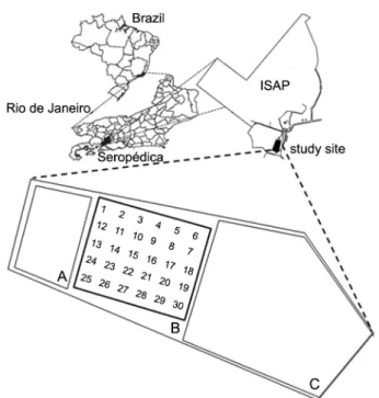
An area of 2,502 m2 was cultivated with corn,
where a regular square grid with 10 m spacing was in-stalled. Considering this layout, the experiment consist-ed of 30 sampling locations (Figure 1A, B and C). For each of the 30 sampling locations, Universal Transversa Mercator (UTM) coordinates were measured using a Global Position System with differential correction. Soil samples were collected for soil texture analysis at depths of 0.05, 0.15, and 0.30 m. Soil textural composition was quantified using the sieving and pipette method (Em-brapa, 1997). Furthermore, at each measurement point and at the same soil depth, a total of 90 soil sensors were installed, parallel to the soil surface, and the dielectric constant (Ka) was monitored using time domain reflec-tometry. The volumetric soil water content (SWC) was calculated (cm3 cm−3) using the Topp equation (Topp et
al., 1980). The soil water content was measured for 18 days during the first year (15, 16, 17, 19, 20, 22, 23, 24, 26 Jan; 11, 12, 14, 16, 21, 22, 24, 27 Feb; 3 Mar 2014) and for 9 days during the second year (15, 16, 17, 18 Dec 2014; 5, 7, 10, 12, 19 Jan 2015). The sensors were installed in Jan 2014, remaining there until Mar when they were uninstalled for soil tillage. In Dec 2014 the sensors were reinstalled at the same points. Over the two periods of monitoring, precipitation was measured hourly by an automatic meteorological station located approximately 1000 m from the study area.
Statistical analysis
Descriptive statistics (mean, variance, maximum and minimum value, standard deviation and coefficient of variation) were calculated and used to evaluate the magnitude of data dispersion. Spearman`s rank correla-tion coefficient was calculated with the aim of correlat-ing the soil water content at different times and its rela-tionship to other soil properties.
The relative mean difference (δij) was calculated
and presented graphically in order to show the rank of wettest, driest and mean points in the area for each year. This technique ranks the measurement locations based on the relative difference from the spatial mean (Vachaud et al., 1985). The relative mean difference was calculated as follows (Eq. 1):
δij ij
j S
=∆ Eq[1]
where Δij is calculated by the difference between the surements at each point (i) on day (j) and the mean mea-surement for day (j), and Sjrepresents the field mean soil
water storage for a particular day (j). For each location, the average and standard deviation of δij, were calculated and graphically presented. With this analysis we deter-mined the average, wettest and driest spots. Whether these locations persist over time or not can be detected by the standard deviation of δij. Values of δij close to zero mean that their locations present a soil water content sim-ilar to the field average. Negative values of δij mean that their locations are drier than the field average, while posi-tive values of δij mean that their locations are wetter than the field average. Moreover, the nonparametric Spearman Rank correlation (rs - eq. 2) was applied to evaluate the persistence of spatial patterns of soil water content at dif-ferent times (temporal stability). The Spearman rank cor-relation was calculated as follows:
r R R
N N s i N ij ij = − − − = ′
∑
1 6 1 1 2 ( )²( ) Eq[2]
where Rij is the rank of observed variable at loca-tion i and date j, Rij' is the rank of the same vari-able, at the same location, but at date j', and N is the number of observations at a particular time.
Temporal stability implies a relationship between soil water storage at times t1 and t2. A location that is relatively dry at time t1 compared to other locations will remain relatively dry at time t2. The closer the value of rs
to 1 the more stable the pattern is observed over time. In other words, the rank for soil water content on each day remains similar over time.
The number of soil samples necessary to calculate the mean was determined by Equation 3 (Petersen and Calvin, 1982) as follows:
n t D = ∗ σ2
2 Eq[3]
where t is the critical value of “t” (student); s2 the
vari-ance and D a specified limit. Figure 1 − The study site with vegetable production area (A), the
Results and Discussion
The soil texture and soil water content across the plot
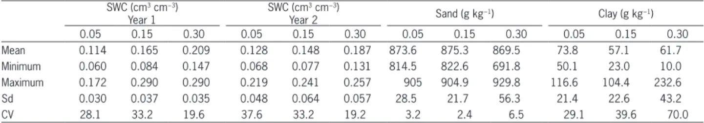
The highest average values of soil water content (SWC) were found at a depth of 0.30 m followed by the 0.15 m and the 0.05 m depths for both years (Table 1). The 0.30 m soil depth was higher in clay content and water retention capacity (Figure 2C). It thus explains, in part, the vertical differences in soil water content. On the other hand, the 0.05 and 0.15 m soil depths are more exposed to evapotranspiration, which reduces soil water content. The exposure to evapotranspiration processes may also explain the highest values for the coefficient of variation (CV) which cause more rapid temporal chang-es of SWC at depths of 0.05 and 0.15 m (Table 1). As reported by Brocca et al. (2007) and Hu et al. (2008), the CV tended to be higher when the soil water content decreased. Therefore, the soil water content was more homogeneous at the deepest layer (0.30 m) and the tem-poral dynamic was more evident close to the surface (Hupet and Vanclooster, 2002; Guber et al., 2008).
The SWC, standard deviation (Sd) and coefficient of variation (CV) also showed a systematic difference between the two periods of the years monitored. The second year presented lower SWC and higher Sd and CV, at the three soil depths, than year 1 (exception only for CV at 0.30 m).
The spatial distribution of sand content at the three soil depths is presented in Figure 2 (A, B and C, respectively). The dominant texture class, at the three sample depths, was sandy and greatly influenced the other soil attributes, resulting in low water retention and water availability. Sandy soil has higher macropores and lower specific surface areas (SA) than clayed soils. The SA and, therefore, the clay content play important roles in the adsorption and desorption of water molecules. SA plays a dominant role for the adsorption of water mol-ecules, i.e., the surface adsorptive forces greatly affect water retention (Petersen et al., 1996).
Systematically, and at all soil depths, the bottom part of the plot area had higher sand content than the upper part, mainly when compared to the upper left re-gion (higher clay content). The sand contents at 0.05 and 0.15 m were very similar. The higher standard deviation was found at the 0.30 m depth, at 0.05 m it was slightly higher than at 0.15 m. This may result from the fact that
the 0.30 m soil depth is coincident to the upper bound-ary of a transitional zone to an argillic horizon (B) in this Alfisoil. The minimum value of sand content at the 0.30 m soil depth confirm this soil characteristic (Table 1).
Table 1 − Descriptive statistics for soil water content and texture. SWC (cm3 cm−3)
Year 1
SWC (cm3 cm−3)
Year 2 Sand (g kg
−1) Clay (g kg−1)
0.05 0.15 0.30 0.05 0.15 0.30 0.05 0.15 0.30 0.05 0.15 0.30
Mean 0.114 0.165 0.209 0.128 0.148 0.187 873.6 875.3 869.5 73.8 57.1 61.7
Minimum 0.060 0.084 0.147 0.068 0.077 0.131 814.5 822.6 691.8 50.1 23.0 10.0
Maximum 0.172 0.290 0.290 0.219 0.241 0.257 905 904.9 929.8 116.6 104.4 232.6
Sd 0.030 0.037 0.035 0.048 0.064 0.057 28.5 21.7 56.3 21.4 22.6 43.2
CV 28.1 33.2 19.6 37.6 33.2 19.2 3.2 2.4 6.5 29.1 39.6 70.0
SWC = soil water content; Sd = standard deviation; CV = coefficient of variation.
Temporal and spatial variability of SWC and its correlation over time
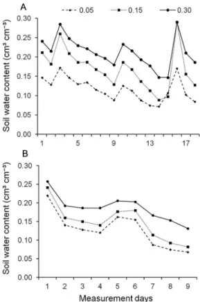
The average values of the SWC, considering the 30 monitored points, along the two periods of monitor-ing and, at the three soil depth, are presented in Fig-ure 3A and B. At all soil depths, the SWC increased and decreased simultaneously, following a similar pattern of variation. The average values of SWC at 0.30 m soil depth were always higher than at 0.15 and 0.05 m, re-spectively. In general, the SWC throughout the second year monitored was lower than the first year.
During the first year of monitoring (Figure 3A), the fourteenth (21 Mar 2014) and sixteenth (24 Mar 2014) sampling day presented the driest and wettest SWC, respectively. After the fourteenth day of mea-surement precipitation events occurred, 3.8 mm, 10.2 mm, 59.6 mm and 2 mm on following days (Figure 4A). It explains the increase in SWC. From the sixteenth to the seventeenth day (27 Mar 2014), the SWC decreased quickly manifesting how fast the water dynamics are in the soil layer evaluated, which reflected the combined effect of the high sand content and evapotranspiration. Due to the high sand content, high volumes of macro-pores and low surface area, this soil has low water re-tention capacity. The macropores can cause rapid water movement (Beven and Germann, 1982). By the four-teenth day the water lamina at the 0-0.30 m soil layer
was 30.7 mm. After a rainfall of 81.2 mm, it reached 74.99 mm (sixteenth day) and 2 days later (eighteenth day) it decreased to 39 mm.
In the second period of SWC monitoring (Figure 3B), the fluctuation in SWC was relatively smaller and on days 1, 5 and 6, the highest soil water contents were observed. Clearly, the precipitation during this year was lower than in the first year which can be seen in the maximum precipitation values. The value of precipita-tion in the second year reached a maximum of only 11 mm, while in the first year the majority of precipitation events surpass 11 mm, achieving a maximum of 88.6 mm (Figure 4B).
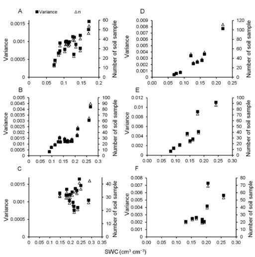
The variance decreased when the soil water con-tent decreased at the 0.05 and 0.15 m soil depthfor both years (Figure 5 A, B, D and E). This result implies that the soil water content distribution was more homoge-neous under dry conditions. Therefore, the number of soil samples necessary to determine the mean of soil wa-ter under dry conditions will be lower than under wet conditions (Figure 5A, B, D and E). For 0.30 m this cor-relation was not clear (Figure 5C and F).
The information about the behavior of the SWC at each of the 30 points monitored during the 2 years is shown in Figures 6A and B (ranked relative mean differ-ence) and Figure 7A and B (wettest, average and driest points). The points were classified as the average, the driest (considering a moisture value of less than 10 % of the mean), and the wettest (considering moisture value
Figure 4 − Values of precipitation for whole measurement period, for first (A) and second (B) year. Numbers above of points are respective measurement days of soil water content (SWC). Numbers under the “x” axis represents the monitoring period, 46 days for the first year and 36 for the second.
of more than10 % of the mean) in the study plot. For the first year of monitoring, points 30, 18 and 17 exhibited soil water content 30 %, 26 % and 21 % drier than the average soil moisture, respectively. On the other hand, points 26, 11 and 25 showed 44 %, 36 % and 21 % wetter than the average soil moisture. At points 8, 1, 5, 7, 20, 22 the soil water content was close to the average value (Fig-ure 6A). Those points close to the average represent the Figure 5 − Correlation between soil water content (SWC) and variance; soil water content and number of soil sample (n) during the year 1 (0.05
m, A; 0.15 m, B; 0.30 m, C) and year 2 (0.05 m, D; 0.15 m, E; 0.30 m, F).
Figure 6 − Ranked mean relative difference (δij) for soil water content for first (A) and second year (B).
mean soil water content. In other words, measuring soil water content at these points provides an idea about the mean soil water content of the area on a particular day.
For the second year, points 18, 8, 17 and 19 exhib-ited soil water contents 47 %, 38 %, 31 % and 31 % drier than the average soil water content, respectively. Points 22, 25, 13, 12 showed 62 %, 52 %, 46 % and 36 % wetter than the average. At points 6, 14, 28, 10 the soil water contents were close to the average (Figure 6B). Points 18 and 25 remained between the three driest and wet-test points for both years, respectively. Thus we can use these points to monitor the driest and wettest values for soil water content, respectively, on any particular day.
In summary, points 18 and 25 show temporal sta-bility and represent the driest and the wettest water con-tent in the study site, respectively. However, the points representing average soil water content were not the same for the first and the second year. Van Pelt and Wi-erenga (2001) made comparisons between years and not-ed that temporal stability also changnot-ed over the years. These authors considered that removal and reinstalla-tion of soil water content sensors could influence the measurements and thus cause lack of continuity. Fur-thermore, tillage practices change the soil structure and, consequently, can change the dynamics of hydric regime at a specific point or region of the field.
When considering the spatial positions of the driest and wettest points, we observed that these points were close to each other (Figure 7A and B). Many studies have shown the soil water content to be spatially dependent. Generally, samples taken close to each other show more similarities (Nielsen and Wendroth, 2003). Brocca et al. (2007) and Vieira et al. (2008) measured soil water content with time domain reflectometer probes and obtained the spatial dependence of soil water content for the dates
mea-Table 2 − Matrix of Spearman Rank correlation coefficient of soil water storage measurements for 0.00-0.30 m during the first year. Day 1 Day 2 Day 3 Day 4 Day 5 Day 6 Day 7 Day 8 Day 9 Day10 Day11 Day12 Day13 Day14 Day15 Day16 Day17 Day18 Day 1 1.00
Day 2 0.94 1.00 Day 3 0.52 0.60 1.00 Day 4 0.55 0.70 0.80 1.00 Day 5 0.56 0.72 0.71 0.98 1.00 Day 6 0.56 0.73 0.68 0.95 0.97 1.00 Day 7 0.51 0.70 0.56 0.87 0.92 0.96 1.00 Day 8 0.46 0.66 0.52 0.84 0.89 0.94 0.98 1.00 Day 9 0.41 0.60 0.39 0.76 0.81 0.87 0.95 0.97 1.00 Day10 0.48 0.63 0.80 0.86 0.82 0.83 0.75 0.73 0.66 1.00 Day11 0.43 0.57 0.70 0.81 0.78 0.80 0.76 0.74 0.69 0.97 1.00 Day12 0.37 0.51 0.52 0.63 0.62 0.67 0.69 0.70 0.67 0.84 0.91 1.00 Day13 0.35 0.50 0.47 0.62 0.62 0.64 0.70 0.70 0.71 0.75 0.85 0.92 1.00 Day14 0.33 0.47 0.36 0.55 0.56 0.64 0.70 0.71 0.74 0.67 0.79 0.86 0.93 1.00 Day15 0.25 0.35 0.36 0.43 0.42 0.49 0.54 0.54 0.58 0.57 0.69 0.75 0.86 0.93 1.00 Day16 0.62 0.67 0.80 0.87 0.80 0.77 0.66 0.61 0.51 0.82 0.75 0.53 0.49 0.43 0.33 1.00 Day17 0.34 0.50 0.65 0.88 0.85 0.84 0.82 0.80 0.74 0.87 0.87 0.73 0.69 0.65 0.54 0.80 1.00 Day18 0.21 0.37 0.48 0.66 0.63 0.63 0.69 0.66 0.66 0.66 0.71 0.71 0.71 0.68 0.64 0.51 0.82 1.00 Spearman Rank correlations are significant in bold (alpha 0.05).
sured. However, spatial dependence changes over time according to the magnitude of soil water content (Wen-droth et al., 1999; Shume et al., 2003; Veronese Júnior et al., 2006; Vieira et al., 2008). Low correlation ranges or spatially random correlation behavior were often associ-ated with both rainfall events and water redistribution in internal drainage. It may be the result of changes in the dominating factors in surface processes (evapotranspira-tion, lateral water flow, values of hydraulic gradient) in different soil water content (Greminger et al., 1985; Wen-droth et al., 1999; Hu et al., 2008).
If we consider the mean soil water content during the first year, 0.16 cm3 cm−3, the three wettest points (26,
11, 25) exhibited a soil water content 0.44, 0.36, 0.21 above the mean (Figure 6A), or 0.23, 0.21 and 0,19 cm3
cm−3 above the mean. The three driest points (30, 18,
17, respectively) exhibited soil water contents 0.30, 0.27, 0.21 below the mean, or 0.11, 0.12 and 0.13 cm3 cm−3
below the mean, respectively. Therefore, the magnitude of difference of soil water content at wettest and driest points was very large reaching 0.12 cm3 cm−3, if we
com-pare points 26 and 30.
Figure 8 − Relationship between soil water content (SWC) and Spearman's rank correlation (SRC) for 0.05 m (A), 0.15 m (B) and 0.30 m (C) for first year and 0.05 m (D), 0.15 m (E) and 0.30 m (F) for second year.
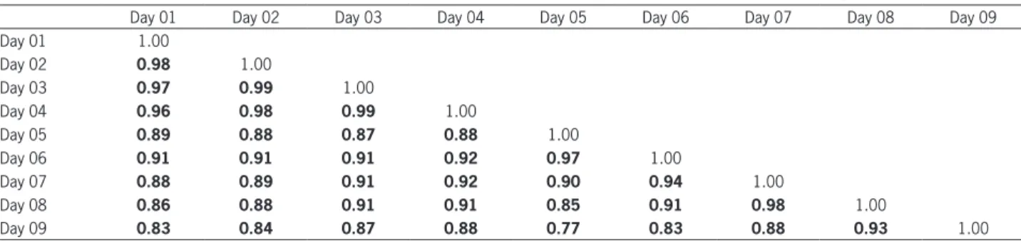
Table 3 − Matrix of Spearman Rank correlation coefficient of soil water storage measurements for 0.00-0.30 m during the second year.
Day 01 Day 02 Day 03 Day 04 Day 05 Day 06 Day 07 Day 08 Day 09
Day 01 1.00
Day 02 0.98 1.00
Day 03 0.97 0.99 1.00
Day 04 0.96 0.98 0.99 1.00
Day 05 0.89 0.88 0.87 0.88 1.00
Day 06 0.91 0.91 0.91 0.92 0.97 1.00
Day 07 0.88 0.89 0.91 0.92 0.90 0.94 1.00
Day 08 0.86 0.88 0.91 0.91 0.85 0.91 0.98 1.00
Day 09 0.83 0.84 0.87 0.88 0.77 0.83 0.88 0.93 1.00
Spearman Rank correlation are significant in bold (alpha 0.05).
Spearman's rank correlation increased again. This be-havior was observed for all depths. Spatial and temporal series follow a similar pattern over time as the soil dries out (Wendroth et al., 1999).
According to the findings of this study, the dry season (from May to Aug in the study site) present the lowest SWC variation, which means a longer interval with simi-lar spatial patterns of SWC distribution. In this case, the interval between measurements of SWC could be lon-ger and the number of measurements could be lower. In the wettest season (Sept to Apr), when the precipitation and evapotranspiration are higher, the SWC will change more frequently, requiring shorter intervals between soil water measurements.
Considering the above, in the first year (Figure 8A, B and C), the period between days 3 and 9 which highlights the interval between days 4 and 6, the Spear-man rank correlation coefficients remained highest for a long period of time, while the SWC decreased, for all soil depths, namely, at about 0.084 cm3 cm−3 for the 0.05
m depth, 0.13 cm3 cm−3 for the 0.15 m depth and 0.105
cm3 cm−3 for the 0.30 m depth. In proportional terms,
the SWC decreased around 48 % at 0.05 m, 50 % at the 0.15 m depth and 37 % at the 0.30 m depth. The high values for Spearman rank correlation mean that SWC distribution in the field showed a pattern connecting these days (temporal stability). Thus, by measuring the water content at average points (points 8, 1, 5, 7, 20 and 22) we could estimate the SWC at other points up to day 9. On the other hand, if we consider day 1 as a refer-ence, the decreasing Spearman rank correlation coeffi-cients show that after day 3 the measurements of that day were no longer related to day 1 (Figure 8A, B and C). In this case the spatial distribution of SWC on day 3 was not the same as on day 1. This second example shows heterogeneous Spearman rank correlation coefficients during the wet season, which demands more frequent measurements in space and time. The data of the second year (Figure 8D, E and F), despite being also taken in the wet season, can give an indication of what would have happened in the dry season. During the second period of monitoring, both the rain and the SWC were at their lowest. In this case, considering day one as a reference for SWC measurement (Table 3), the Spearman rank co-efficient value would remain high up to day 4 when it decreased before it increased again.
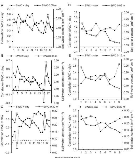
The correlation between SWC and clay content over time
The Pearson correlation coefficient between soil water contents and clay content varied not only at dif-ferent depths on the same day but also over time for both years (Figure 9A, B, C, D, E and F). On certain days correlation was positive and significant while on others correlation decreased and became insignificant. This phenomenon was associated with the magnitude of soil water content. When the soil dried after a rain-fall, the correlation coefficient increased. Greminger et al. (1985) measured soil water content in a transect over time and found crosscorrelation between sand and soil water pressure head under dry conditions but under wet conditions the crosscorrelation coefficients were small and usually insignificant. We observed this behavior in
the first year at the 0.05 m depth for the first ten sam-pling days. At the 0.30 m depth this behavior was evi-dent for the entire period. The drier soil showed higher correlation coefficients values at 0.30 m. At the 0.15 m depth no correlation was observed between SWC and soil texture (Figure 9A, B and C).
For the second year, the correlation tended to in-crease, once the soil became dry after the end of a rain event. The correlation was high for 0.30 m at all days, except on days 5 and 6 (Figure 9F) after the soil became wet. At 0.15 m the correlation coefficient was weak (Fig-ure 9E). Thus, the distribution of clay content in the area may explain the distribution of water at the 0.30 m soil depth. Probably, the behavior of water distribution in the upper layers was more influenced by the evapotrans-piration process and the contents of soil organic matter. Moreover, as the first 0.20 m soil depth is more frequent-ly plowed, it can also influence soil water distribution, and consequently reduce correlation between SWC and clay content.
These results imply that the influence of soil clay content depends on soil water content and whether the soil is in a drying or wetting phase. Total soil water po-tential consists of four components: matric, gravitation, pressure and osmotic potential. The importance of each component of total soil water potential changes with soil water content. When the soil gets wet during a rainfall, the gravitational potential is important because the soil water is “free” and in this case it is drained by macro-pores. In this case the soil macroporosity would govern the distribution of soil moisture. As the soil becomes dry, the soil surface and water surface interaction increase; therefore, at this soil moisture level the clay content (ad-sorptive forces) and micropores (capillary forces) govern the soil water distribution. Soil matric potential gains in importance. This physical phenomenon explains the change of correlation between soil water content and soil mineral particles.
Conclusions
Our findings indicate that the soil water content showed temporal stability between year 1 and 2 for both the driest and the wettest points in the study site. However, this pattern was not followed for the points representing the average soil water content. In this case we cannot use the average points of year 1 to estimate soil water in year 2. Probably the removal and reinstalla-tion of sensors, as well as the tillage management of the study site, influenced the measurements and therefore contributed to the lack of continuity.
Figure 9 − Values of correlation between soil water content × clay and soil water content (SWC) for 0.05 m (A), 0.15 m (B) and 0.30 m (C) at first year and 0.05 m (D), 0.15 m (E) and 0.30 m (F) at second year.
In any specific year of monitoring, the decrease in Spearman coefficient rank was associated with rainfall events, showing a cyclical pattern. Soon after rainfall the temporal stability decreases and when the soil be-gins to dry out, Spearman rank correlation increases again. Due to this cyclical pattern, for wetter periods it is necessary to intensify the number of sensors and the period of SWC monitoring in the area.
The Spearman correlation between soil water and clay contents varied not only according to depth but also according to soil moisture. Correlation is lower in the upper layers, where it is influenced more by tillage practices, soil organic carbon changes and the evapo-transpiration process. When the soil became drier, mainly in the 0.30 m soil layer where the clay content is higher, correlation increased due to the preponder-ance of adsorptive and capillary forces over soil water distribution.
Acknowledgements
The authors extend thanks to the Coordination for the Improvement of Higher Level Personnel - CAPES, un-der the Science without Borun-ders Program, for providing funds through the “Special visiting researcher program” (number 152140). CAPES PVE-8888.030464/2013-01.
References
Alvares, C.A.; Stape, J.L.; Sentelhas, P.C.; Gonçalves, J.L.M; Sparovek, G . 2013. Köppen's climate classification map for Brazil. Meteorologische Zeitschrift 22: 711-728.
Beven, K.; Germann, P. 1982. Macropores and water flow in soils. Water Resources Research 18: 1311-1325.
Ceddia, M.B.; Vieira, S.R.; Villela, A.L.O.; Mota, L.S.; Anjos, L.H.C.; Carvalho, D.F. 2009. Topography and spatial variability of soil physical properties. Scientia Agricola 66: 338-352. Empresa Brasileira de Pesquisa Agropecuária [EMBRAPA]. 1997.
Soil Analysis Methods = Manual de Métodos de Análise de Solo. 2ed. Centro Nacional de Pesquisa de Solos, Rio de Janeiro, RJ, Brazil (in Portuguese).
Greminger, P.J.; Sud, Y.K.; Nielsen, D.R. 1985. Spatial variability of field-measured soil-water characteristics. Soil Science Society of America Journal 49: 1075-1082.
Guber, A.K.; Gish, T.J.; Pachepsky, Y.A.; van Genuchten, M.T.; Daughtry, C.S.T.; Nicholson, T.J.; Cady, R.E. 2008. Temporal stability in soil water content patterns across agricultural fields. Catena 73: 125-133.
Hu, W.; Shao, M.A.; Wang, Q.J.; Reichardt, K. 2008. Soil water content temporal-spatial variability of the surface layer of a Loess Plateau hillside in China. Scientia Agricola 65: 277-289. Hu, W.; Shao, M.; Han, F.; Reichardt, K.; Tan, J. 2010. Watershed
scale temporal stability of soil water content. Geoderma 158: 181-198.
Hupet, F.; Vanclooster, M. 2002. Intraseasonal dynamics of soil moisture variability within a small agricultural maize cropped field. Journal of Hydrology 261: 86-101.
Kachanoski, R.G.; Jong, E. 1988. Scale dependence and the temporal persistence of spatial patterns of soil water storage. Water Resources Research 24: 85-91.
Letey, J. 1985. Relationship between soil physical properties and crop production. Advances in Soil Science 1: 277-294.
Nielsen, D.R.; Wendroth, O. 2003. Spatial and Temporal Statistics-Sampling Field Soils and Their Vegetation. Catena Verlag GMBH, Reiskirchen, Germany.
Pachepsky, Y.A.; Guber, A.K.; Jacques, D. 2005. Temporal presistence in vertical distributions of soil moisture contents. Soil Science Society of America Journal 69: 347-352.
Petersen, R.G.; Calvin, L.D. 1982. Sampling. p. 33-51. In: Klute, A. Methods of soil analysis. Part 1. Physical and mineralogial methods. Madison, WI, USA.
Petersen, L.W.; Mouldrup, P.; Jacobsen, O.H.; Rolston, D.E. 1996. Relations between specific surface area and soil physical and chemical properties. Soil Science 161: 9-21.
Reynolds, S.G. 1970. Gravimetric method of soil moisture determination III. Journal of Hydrology 11: 288-300.
Shume, H.; Jost, G.; Katzensteiner, K. 2003. Spatio-temporal analysis of the soil water content in a mixed Norway spruce (Picea abies (L.) Karst.) – European beech (Fagus sylvatica L.) stand. Geoderma 112: 273-287.
Silva, A.P.; Nadler, A.; Kay, B. 2001. Factors contributing to temporal stability in spatial patterns of water content in the tillage zone. Soil Tillage Research 58: 207-218.
Souza, E.R.; Montenegro, A.A.D.A.; Montenegro, S.M.G.; Matos, J.D.A. 2011. Temporal stability of soil moisture in irrigated carrot crops in Northeast Brazil. Agricultural Water Management 99: 26-32.
Starr, G.C. 2005. Assessing temporal stability and spatial variability of soil water patterns with implications for precision water management. Agricultural Water Management 72: 223-243.
Topp, G.C.; Davis, J.L.; Annan A.P. 1980. Eletromagnetic determination of soil water content: measurements in coaxial transmission lines. Water Resources Research 16: 574-582. Vachaud, G.; Silans, A.P.; Balabanis P.; Vauclin, M. 1985. Temporal
stability of spatially measured soil water probability density function. Soil Science Society of America Journal 49: 822-828. Van Pelt, R.S.; Wierenga, P.J. 2001. Temporal stability of spatially
measured soil matric potential probability density function. Soil Science Society of America Journal 65: 668-677.
Veronese Júnior, V.V.; Carvalho, M.P.; Dafonte, J.; Freddi, O.S.; Vidal Vázquez, E.; Ingaramo, O.E. 2006. Spatial variability of soil water content and mechanical resistance of Brazilian ferralsol. Soil Tillage Research 85: 166-177.
Vieira, S.R.; Grego, C.R.; Topp, G.C. 2008. Analyzing spatial and temporal variability of soil water content. Bragantia 67: 463-469.
Wang, X.; Pan, Y.; Zhang, Y.; Dou, D.; Hu, R.; Zhang, H. 2013. Temporal stability analysis of surface and subsurface soil moisture for a transect in artificial revegetation desert area, China. Journal of Hydrology 507: 100-109.
Wendroth, O.; Pohl, W.; Koszinski, S.; Rogasik, H.; Ritsema, C.J.; Nielsen, D.R. 1999. Spatio-temporal patterns and covariance structures of soil water status in two Northeast-German field sites. Journal of Hydrology 215: 38-58.