Spatial-Temporal Dynamics of
High-Resolution Animal Networks: What Can We
Learn from Domestic Animals?
Shi Chen1*, Amiyaal Ilany2, Brad J. White3, Michael W. Sanderson3, Cristina Lanzas1
1Department of Population Health and Pathobiology, North Carolina State University, Raleigh, NC, 27607, United States of America,2Department of Biology, University of Pennsylvania, Philadelphia, PA, 19104, United States of America,3College of Veterinary Medicine, Kansas State University, Manhattan, KS, 66506, United States of America
Abstract
Animal social network is the key to understand many ecological and epidemiological pro-cesses. We used real-time location system (RTLS) to accurately track cattle position, analyze their proximity networks, and tested the hypothesis of temporal stationarity and spatial homo-geneity in these networks during different daily time periods and in different areas of the pen. The network structure was analyzed using global network characteristics (network density), subgroup clustering (modularity), triadic property (transitivity), and dyadic interactions (corre-lation coefficient from a quadratic assignment procedure) at hourly level. We demonstrated substantial spatial-temporal heterogeneity in these networks and potential link between inrect animal-environment contact and diinrect animal-animal contact. But such heterogeneity di-minished if data were collected at lower spatial (aggregated at entire pen level) or temporal (aggregated at daily level) resolution. The network structure (described by the characteristics such as density, modularity, transitivity, etc.) also changed substantially at different time and locations. There were certain time (feeding) and location (hay) that the proximity network structures were more consistent based on the dyadic interaction analysis. These results re-veal new insights for animal network structure and spatial-temporal dynamics, provide more accurate descriptions of animal social networks, and allow more accurate modeling of multi-ple (both direct and indirect) disease transmission pathways.
Introduction
Analysis of animal networks is essential to predict animal behavior, characterize sociality, and investigate many ecological and evolutionary processes, including disease transmission [1]. Many aspects of animal social networks change through time, from global network structure to basic dyadic (between two individuals) interactions [2,3]. There are two basic types of tempo-ral dynamics on the network: the network structure (intrinsic changes in the network struc-ture), and flow dynamics on the network (e.g. disease transmission, substance and energy flow OPEN ACCESS
Citation:Chen S, Ilany A, White BJ, Sanderson MW, Lanzas C (2015) Spatial-Temporal Dynamics of High-Resolution Animal Networks: What Can We Learn from Domestic Animals? PLoS ONE 10(6): e0129253. doi:10.1371/journal.pone.0129253
Academic Editor:Renaud Lambiotte, University of Namur, BELGIUM
Received:November 9, 2014
Accepted:May 6, 2015
Published:June 24, 2015
Copyright:© 2015 Chen et al. This is an open access article distributed under the terms of the
Creative Commons Attribution License, which permits unrestricted use, distribution, and reproduction in any medium, provided the original author and source are credited.
Data Availability Statement:Relevant data are available at Figshare. DOI:http://dx.doi.org/10.6084/ m9.figshare.1416302.
in food webs [3]). These two types of temporal dynamics, however, are not mutually exclusive as flow dynamics are also closely dependent on network structure changes, and vice versa. A static description of the network may not be able to accurately capture the comprehensive net-work structure and flows [4,5].
Recent studies have progressed in developing both concepts and techniques for temporal network dynamics. Temporal network dynamics can take place at different scales: at entire net-work/global level (how the global network characteristics, such as network density, varies over time), at sub-graph level (how clusters of individuals form and change), at the triadic level (how the transitivity in the triad changes among three vertices), and at the dyadic level (how the relationship of each pair of individuals in the network evolves). Meanwhile, novel computa-tional tools have also been developed to detect and quantify network characteristics and tem-poral network dynamics, such as quadratic assignment procedure (QAP [6]), exponential random graph model [7–9], modularity detection [10,11], transitivity test [12], and network comparison across space and time [13,14].
Temporal networks have been applied to various wild animal populations, from primates to insects, including cyclic population structure in female African baboons [15], social niche stabili-ty in primates [16], dynamics of social networks among Asian elephants [17], social system re-structure and dynamics in dolphins [18,19], social network and genetic structure in spotted hyenas [20], social cohesion of marmots remaining at home [21], social network evolution and kin cluster in manakin birds [22,23], dynamic social networks in guppy fish [24,25], temporal and individual variation in social ant colonies [26,27], and triad dynamics in the rock hyrax [28].
A major problem for studies in wildlife ecology is that most of the wild animals are difficult to track individually and continuously with a high sampling rate (resolution) hence the result-ing networks are at low temporal resolution, usually at daily level or longer. Furthermore, spa-tial heterogeneity is also important in animal social networks but often untraceable or ignored [3]. These difficulties substantially hinder the utilization of temporal networks in ecology. These problems can be overcome in studies of networks of domestic animals. Cattle, as many other ungulates, present social interactions such as exploratory behavior, recognition, commu-nication (especially tactile commucommu-nication), and peer bonding [29]. Although quantitative de-scriptions of cattle social networks are still uncommon, dynamic social networks have been recorded in both dairy and beef cattle populations [30–32].
Cattle are usually housed in a confined area so that their position can be explicitly and accu-rately tracked by real-time location system (RTLS) in order to construct ultra-high resolution networks (at second and centimeter resolution temporally and spatially), thus the complete network can be accurately described. Spatial heterogeneity also plays an important role in net-work dynamics [33,34], and data at high-resolution for cattle social networks can facilitate bet-ter understanding of the complicated spatial-temporal dynamics [32]. Furthermore, the group size of a cattle population is generally constant (excluding immigration and emigration, as op-posed to wild animal populations), thus allowing for some computational analysis (e.g. QAP which usually requires the same set of individuals/vertices in the networks). Thus cattle are suitable candidates to study spatial-temporal dynamics of animal networks that can provide in-sight on the dynamics of such networks in other domestic and non-domestic species.
We here construct high-resolution cattle proximity networks accounting for both temporal (at hourly level in a day) and spatial (different areas in the pen, e.g. feeding bunk, water supply, and hay bunk) heterogeneities. We comprehensively and quantitatively compare and contrast how the network structure changes at different network topology levels, from global network characteristics, to subgraph, triadic, and down to the dyadic interactions, at different time and area, and demonstrate the spatial-temporal heterogeneity at these different levels in a cattle net-work. This enhances our understanding of animal network dynamics, develops more realistic
description and characterization of social networks, and facilitates future research such as in-corporating accurate disease transmission models on social networks.
Materials and Methods
Data acquisition and standardization
Real-time animal position data were collected at the research farm of Kansas State University (Manhattan, KS, USA). Three pens of Holstein calves were monitored, with 21, 21, and 27 calves in pens #1 to #3, respectively. The entire pen is partitioned into four exclusive areas: around the grain bunk (5m2), the hay bunk (5m2), the water trough (3m2), and all the other areas in the pen (187m2). Each calf was continuously monitored from August 11, 2011, to Au-gust 18, 2011, using a wide-band radio frequency tag (Ubisense Series 7000 Compact Tag, Ubi-sense Group, UK) attached to its ear. The tag transmitted ultra wide-band signals to seven receivers around the pens; the receivers then transferred data to a central computer that logs the 2-dimensional (X-Y coordinates) position data. This real-time location system (RTLS) was accurate (up to 0.01 m in spatial resolution and 1s in temporal resolution) and did not disturb the animals nor change their normal behavior. The original position data reported by the tags of each animal were aggregated to 10-s resolution. Hence, in each day, each animal would have 8,640 2-dimensional data points recording its location (24 h/d×60 min/h×6 data/min). The de-tailed data acquisition and standardization processes are presented in our previous work with indirect and direct contact independently [31,32]. All the animal experiments associated with this manuscript were approved by and complied with the animal regulation policy of the Kan-sas State University.
Network construction
First, the cattle network was generated based on the cattle position data in every hour (a total of 192 hours in this study, thus 192 hourly networks) using a 0.3m threshold distance, as de-scribed in our previous work [32] (this work did not take specific spatial areas, e.g. grain, hay, and water into consideration). We use spatial proximity to approximate social closeness in this study (thus proximity network is an approximate to the real social network) because the ani-mals are in a confined area. Then, whenever a direct contact occurs, the positions of the pair are determined and such direct contact is attributed to one of the four areas, using the same 0.3m threshold distance. For example, if two calves are in contact and their position falls within the 0.3m threshold distance of the grain bunk, this direct contact occurs around the grain bunk. Occasionally, a direct contact can be attributed to more than one area: consider a pair of cattle in contact with animaliwithin threshold distance to the grain bunk but animaljat the general pen floor. In this situation, priority is given to identify the contact as being associated with the more specific areas (e.g. grain, hay, and water) than the general pen floor, and this contact is assumed to occur at the more specific area. Note that grain, hay, and water them-selves in the study pen are sufficiently spatially separated apart that no direct contacts can occur simultaneously in two of them.
The spatially-complete network was partitioned to four spatially-explicit networks repre-senting four different areas in the pen in each hour. These networks are weighted networks (i.e. the values in the adjacency matrixMare not binary but assigned numerical values for the num-ber of contacts). For example, if the value ofMijism, it indicates that two cattleiandjhave a
total ofmcontacts within that hour. In this study we assume an undirected network such that Mij=Mji(animalicontacting animaljimplies animaljcontacting animali), such thatMis a
basis using the same 0.3m threshold distance, and the time series of indirect contact structure is calculated for these specific areas.
As shown later in the results section, the regular feeding activity (twice a day around 8–9am and 2–3pm, shortened as 8am and 2pm hereafter; food is supplied at the grain bunk) signifi-cantly increases cattle contacts during these periods. Our observations also show cattle usually gather around hay to ruminate shortly after feeding. Thus in each day the feeding time (8am and 2pm) is separated from all other non-feeding time. We first investigate the potential cou-pling and synchronization between indirect contact (with grain, water, and hay) and direct contact using time series analysis and spectrum analysis. The time series (at hourly level) tween indirect and direct contact are plotted for the entire 192-h period. The coherency be-tween indirect and direct contact is computed and plotted to quantify such synchronization. If the mean frequency coherency is above certain threshold (sampling frequency) then there is significant correlation between the two (direct and indirect contact) time series. This step is necessary to reveal temporal heterogeneity in network structure and its potential cause. Then we characterize and compare the network structure dynamics at different times of day and at different areas in the pen to delineate the spatial-temporal heterogeneities in the network.
Network characterization and comparison
A range of properties and statistics are used to characterize the hourly network topological struc-ture, from a global level down to dyadic interactions. The network density is one of the most im-portant and common measure of networks at a global level. In our study system (weighted network), the network density is proportional to the total number of contacts in each hour. The network density is bracketed between 0 and 1, where 0 indicates no contact in that time period (1-h) at all and 1 representing a fully connected network (i.e. each pair of vertices is connected).
Furthermore, the vertices in the network (in our study system, the cattle) can show a cluster-ing pattern and form groups. Modularity measures the strength of the division into clusters/ groups. Modularity can be positive or negative, and a larger positive value indicates stronger clustering pattern [35]. At the triadic level (three vertices), transitivity, also known as the global clustering coefficient, measures to what extent vertices tend to cluster together [12]. The means and standard errors of modularity and transitivity are also obtained from these networks.
In order to compare network change over time and across space at the dyadic level (two ver-tices, i.e. whether two cattle consistently act together), the QAP is applied. The QAP correlation is an extension of common Pearson’s correlation, and measures how dyadic interaction changes through time for different networks with the same set of vertices. A larger QAP corre-lation indicates more consistent and stable dyadic interaction between two networks at differ-ent times. As indicated before, the time (hour) of day is considered either“feeding”(F) or “non-feeding”(N). For all the 192 observed networks for each area, there are a total of 16 net-works during feeding time (8am/2pm, for 8 days) and 176 for non-feeding time. The QAP is applied between each pair of any two networks during feeding time (a total of 1615/2 = 120
pairsFF), between each pair of networks during non-feeding time (a total of 15,400 pairsNN), and between each pair of networks in feeding and non-feeding times (a total of 1408 pairsFN). All these QAP correlation values are compared between different time periods of the day as well as for different areas in order to reveal dyadic interaction changes. All the analyses were performed inR3.1.0, with thestatnetpackage (version 1.90).
Results
contact between cattle and grain, water, and hay for Pen #1 as an example (Fig 1). The time series of direct contact show substantial diurnal cycle, and the time series between direct and indirect contacts at grain and hay (upper and lower panels, respectively) are significantly coupled, which is supported by the coherency plot in the right panels ofFig 1(potential synchronization occurs since the solid black line is above the red significance level). For instance, the coherency plot for direct contact and indirect contact with grain shows a peak (must be above the red significance level) at around 0.2, which corresponds to an approximately 5-h synchronization between direct contact and indirect contact with grain. However the time series between direct and indirect con-tact with water (middle panel) are not significantly correlated (the solid black mean coherency line does not exceed the significance level, the red horizontal line). Pen #2 and pen #3 have simi-lar results as pen #1 that direct contact is significantly correlated to indirect contacts with grain and hay, but not with water (though not shown in the figure). These results show that cattle net-work density changes significantly within a day, and feeding activity promotes clustering (thus more dense networks) around grain and hay, while drinking is not likely a key factor for network changes. These results indicate that there is neither temporal stationarity nor spatial homogenei-ty in this high-resolution cattle network (number of contacts). Explicit examples of the real cattle networks with possible modules (clustering) at different time and location are provided inFig 2, illustrating strong temporal-spatial heterogeneity in network structure without quantitative mea-surements: the cattle change their aggregation at grain and water in different time periods (8AM vs 8PM) such as number of contacts and potential cluster. However, temporal heterogeneity Fig 1. Time Series of Indirect Contact (Grain, Water, Hay), Periodogram, and Coherency Plot.Note: The subfigures are for grain (upper), water (middle), and hay (lower), respectively. In these subfigures, the time series plots (left panels) of indirect contact and direct contact show high synchrony (coupling) in grain and hay, as supported by the coherency plots (right panels, solid black line) that have substantial part above the threshold (solid red line). There is no clear pattern of relationship between indirect contact with water and direct contact.
vanishes if we look at the networks around hay and the spatially-complete network, where the two time periods yield similar structured networks.
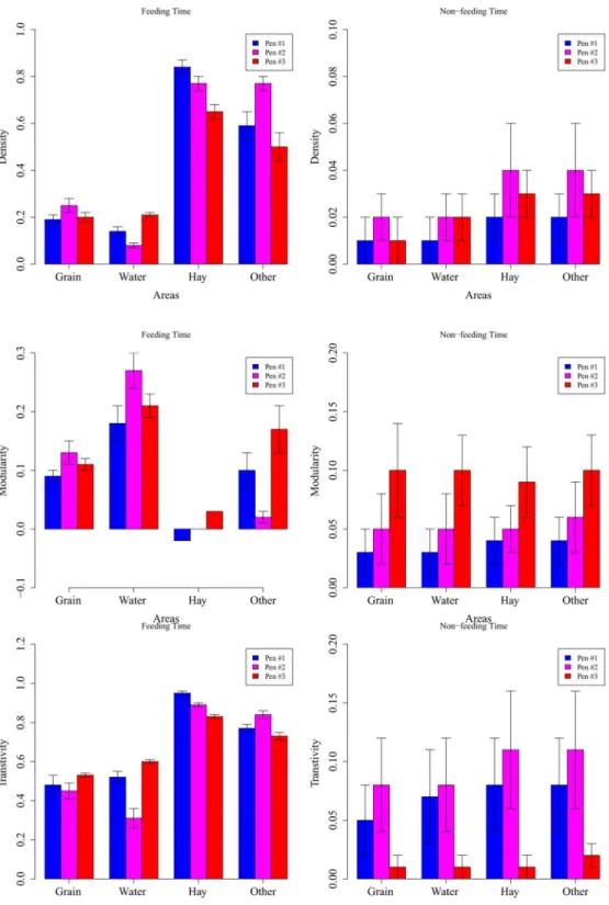
Next, we show three important network measurements (density, modularity, and transitivi-ty, covering levels from the global network structure to dyadic interactions) in different time periods (feeding time were during 8AM-9AM and 2PM-3PM, shortened as 8AM and 2PM thereafter, and non-feeding time were all the other time periods in a day) and in different areas (grain, water, hay, and other pen floor) to explicitly demonstrate the spatial-temporal heteroge-neity (Fig 3). The network density measures at a global network structure level and can be ap-proximated as the number of total contacts. It is not surprising that network density is much higher during feeding time than non-feeding time (Fig 3, first row), as supported by the time series plot inFig 1. Interestingly, the cattle have more contacts around hay than grain even dur-ing feeddur-ing time. This can be explained by the fact that the food supply at the grain is limited and feeding behavior usually only lasts for 15–20 minutes according to our observation31. However the cattle spend significantly longer time (about 45–60 minutes) at hay after feeding to ruminate, and during rumination calves tend to gather together. For the grouping and clus-tering of the networks, results reveal very low modularity value (almost 0) around hay during feeding time, which indicates almost all cattle have some connection with others (Fig 3, 3rd row, left panel). This is very distinct from around the grain, water, and hay during feeding time, and from all areas during non-feeding time.
During feeding time, water area has the largest modularity value (0.18–0.27,Fig 3, 3rdrow). Although the modularity values indicate cattle have some connection with others at hay during feeding time (-0.02–0.03), it is then revealed by the transitivity values that they actually divide into more stable subgroups at hay during feeding time (0.83–0.95,Fig 3, 4throw, left panel). This paradoxical result can be explained by the fact that during feeding time, the cattle tend to cluster into several subgroups and these subgroups are not isolated around hay (i.e. different subgroups Fig 2. Network Structure with Potential Clustering Examples at Different Time and Different Area.
Note: from top to bottom: networks around grain, hay, water, and complete network in the pen. Left: networks aggregated during 8–9AM on Aug. 11. Right: networks aggregated during 8–9PM on Aug. 11. Different colors
indicate potential clustering (subgraph) based on the analysis inRwithstatnetpackage. The thickest line in each network corresponds to the largest number of contacts for that particular area in one hour, thus not directly comparable between different networks. Networks in grain, hay, and water show strong spatial-temporal heterogeneity and distinctive clustering pattern, but such heterogeneity diminishes when aggregated to the complete networks.
Fig 3. Network Structure Characteristics (density, modularity, and transitivity) at Different Time and Different Area.Note: Subfigures are for network structure characteristics: density, modularity and transitivity values, respectively. Left: feeding time (between 8AM-9AM and 2PM-3PM); right: non-feeding time (other time periods). Note all the network characteristics differ significantly between feeding and non-feeding time (left vs right panel in each sub-figure). Spatial heterogeneity (different areas) does not have significant impact during non-feeding time but substantially alter network characteristics during feeding time.
are connected by some“bridge”vertices/individuals). Such a network shows low modularity (i.e. vertices are more or less connected) but high transitivity (i.e. the vertices form distinctive sub-groups). The transitivity values are not substantially different among different areas during non-feeding time. Pen #3 has almost the same transitivity values as pen #1 and pen #2 during non-feeding time, but it yields a smaller transitivity than other pens during non-feeding time. Such pen-level difference can be explained by the fact that transitivity values are generally very low (<0.1) dur-ing non-feeddur-ing time and the pen-level difference is more identifiable.
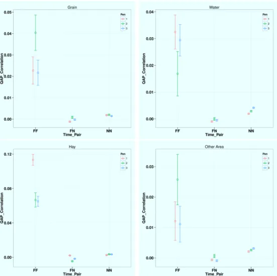
At the dyadic level, the correlations are much stronger (larger quadratic assignment proce-dure, QAP correlation values) between any two feeding time periods (FF) than between any two non-feeding time periods (NN) and between one feeding and one non-feeding time periods (FN), which indicates more stable and consistent dyadic interactions during feeding time at all four locations (seeFig 4). Thus feeding tends to promote and preserve the network structure. For
Fig 4. QAP Correlation Test Results for Different Time Period Pairs at Different Areas.Note: the four sub-figures are for grain, water, hay, and all the other areas, respectively.Findicates feeding time period (8– 9AM, 2–3PM) andNindicates non-feeding time periods. Within each subfigure (the same area) QAP is
significantly larger between two feeding time periods (FF) than between one feeding and one non-feeding time periods (FN) and between two non-feeding time periods (NN). Hay has the much larger QAP correlation during feeding time (FF, valued at about 0.1) than grain (0.03), water (0.02), and all the other area (0.02). Thus the contact network structure especially dyadic interaction is most consistent and stable during feeding time around hay.
different areas during feeding time, hay has significantly higher QAP correlation value (0.10) than grain (0.03), water (0.02), and all other pen floors (0.02), meaning cattle tend to choose their partners and interact with others more consistently around hay during feeding time.
Discussion
Our results clearly reveal that the cattle network has substantial spatial and temporal heteroge-neity. The network structure, from global characteristics to basic dyadic interactions, changes during different times of the day as well as in different areas. Most of the contacts (approximate-ly 60% of total contacts) happen during the feeding time (a total of 2 hours per day, which ac-counts for only 8% of total daily time). Interestingly, hay acac-counts for more direct contacts during feeding time than grain, as can be seen from the network density plot (Fig 2). It also co-incides with our previous finding that cattle spend significantly longer time around hay (about 2 hours per day) than around the grain bunk (about 1 hour per day, 31 Chen et al. 2013). These results show the possible correlation between direct animal-animal contacts and indirect ani-mal-environment contacts. However, the spatial-temporal heterogeneities in the cattle network diminish when the networks are aggregated at lower temporal (e.g. at daily level or above) and spatial (e.g. aggregated at entire pen) resolution. A major challenge to current studies of dynam-ic networks is lack of suffdynam-iciently resolved data, especially for wildlife studies [2,36–39]. Thus cattle (and other domestic animals) serve as an excellent example to study and understand real-time evolution of network structure and potentially shed light on wildlife studies, especially the optimal observation strategy. For instance, researchers can observe animal social network dur-ing specific short period of time while preservdur-ing most of the network structure characteristics Except very specific behavioral interactions, many animal social networks are constructed based on the assumption that spatial proximity reflects social closeness. But this assumption may be incorrect because distance alone (and hence contact) does not necessarily reflect real social ties [3]. Adult cattle have approximately 2m flight distance (an animal will change nor-mal behavior and move if get closer than the flight distance) and young calves have snor-maller flight distance [29]. When a young calf is less than the threshold distance (0.3m in this study) from other calves, it does not necessarily imply the two calves are having some social interac-tion—they may be just randomly passing by each other. The results, especially QAP values, from our study show that the dyadic interaction is unstable and inconsistent during non-feed-ing time periods. Thus, we argue that the some of the contacts durnon-feed-ing non-feednon-feed-ing time are not real social interactions but perhaps just random contacts. During feeding time, social networks formed around hay are much more stable than at the grain bunk. We suggest that during feed-ing time, the cattle need to compete with others for food in the grain bunk thus cannot always eat with an intentionally chosen partner. On the other hand, after feeding the cattle can go with their partner freely to the hay for feeding. Thus the contacts around the grain bunk are facilitat-ed by fefacilitat-eding activity but may not necessarily reflect social ties. It is only the contacts around the hay bunk during feeding time that may attribute to the real social ties. Thus based on the spatial and temporal heterogeneity in the social network, we can categorize the contacts into three types: social, random, and indirect-contact facilitated contact. Our study provides a po-tential way to infer the real social network based on the observed proximity network.
animal and environment and direct contact between animals can be highly synchronized and coupled (especially during feeding time). This enables future research on modeling multiple transmission pathways at the same time, explicitly investigating the relative importance of each transmission pathway (e.g. direct contact, foodborne, waterborne, etc.), and measuring the ef-fects of spatial-temporal heterogeneity with a realistic high-resolution social network.
Acknowledgments
We thank the comments and suggestions from Dr. Louis Gross, National Institute for Biologi-cal and MathematiBiologi-cal Synthesis (NIMBioS), for improvements of this manuscript. This work was conducted with partial funding provided at NIMBioS, an institute sponsored by the U.S. National Science Foundation, the U.S. Department of Homeland Security, and the U.S. Depart-ment of Agriculture through NSF Award # EF-0832858, with additional support from the Uni-versity of Tennessee, Knoxville.
Author Contributions
Conceived and designed the experiments: BW MS. Performed the experiments: BW MS. Ana-lyzed the data: SC. Contributed reagents/materials/analysis tools: SC AI. Wrote the paper: SC CL.
References
1. Croft DP, James R, Krause J. Exploring animal social networks. Princeton University Press; 2008.
2. Blonder B, Wey TW, Dornhaus A, Jame R, Sih A. Temporal dynamics and network analysis. Methods Ecol and Evol. 2012; 3: 958–972.
3. Pinter-Wollman N, Hobson EA, Smith JE, Edelman AJ, Shizuka D, de Silva S, et al. The dynamics of animal social networks: analytical, conceptual, and theoretical advances. Behav Ecol. 2014; 25: 242–
255.
4. Bansal S, Grenfell BT, Meyers LA. When individual behaviour matters: homogeneous and network models in epidemiology. R Soc Interface. 2007; 4: 879–891. PMID:17640863
5. Fefferman N, Ng K. How disease models in static networks can fail to approximate disease in dynamic networks. Phys Rev E. 2007; 76: 031919. PMID:17930283
6. Krackhardt D. Predicting with networks: nonparametric multiple regression analysis of dyadic data. Soc Net. 1988; 10: 359–381.
7. Fienberg SE, Wasserman S. Discussion of An Exponential Family of Probability Distributions for Direct-ed Graphs by Holland and Leinhardt. J Am Stat Assoc. 1981; 76: 54–57.
8. Robins G, Pattison P, Yalish Y, Lusher D. An introduction to exponential random graph (p*) models for social networks. Soc Net. 2007; 29: 173–191.
9. Hunter DR, Goodreau SM, Handcock MS. Goodness of Fit of Social Network Models. J Am Stat Assoc. 2008; 103: 248–258.
10. Newman MEJ. Modularity and community structure in networks. Proc Nat Acad Sci USA. 2006; 103: 8577–8582. PMID:16723398
11. Fortunato S. Community detection in graphs. Phys Rep. 2010; 286: 75–174.
12. Opsahl T, Panzarasa P. Clustering in Weighted Networks. Soc Net. 2009; 31: 155–163.
13. Faust K, Skvoretz J. Comparing networks across space and time, size, and species. Sociol Methodol. 2002; 32: 267–299.
14. Faust K. Very local structure in social networks. Sociol Methodol. 2007; 37: 209–256.
15. Henzi SP, Lusseau D, Weingrill T, van Schaik CP, Barrett L. Cyclicity in the structure of female baboon social networks. Behav Ecol Sociobiol. 2009; 63: 1015–1021.
16. Flack JC, Girvan M, de Waal FBM, Krakauer DC. Policing stabilizes construction of social niches in pri-mates. Nature. 2006; 439: 426–429. PMID:16437106
18. Ansmann IC, Parra GJ, Chilvers BL, Lanyon JM. Dolphins restructure social system after reduction of commercial fisheries. Anim Behav. 2012; 84: 575–581.
19. Cantor M, Wedekin LL, Guimaraes PR, Daura-Jorge FG, Rossi-Santos MR, Simoes-Lopes PC. Disen-tagling social networks from spatiotemporal dynamics: the temporal structure of a dolphin society. Anim Behav. 2012; 84: 644–651.
20. Holekamp KE, Smith JE, Strelioff CC, van Horn RC, Watts HE. Society, demography and genetic struc-ture in the spotted hyena. Mol Ecol. 2012; 21: 613–632. doi:10.1111/j.1365-294X.2011.05240.x
PMID:21880088
21. Blumstein DT, Wey TW, Tang KA. Test of the social cohesion hypothesis: interactive female marmots remain at home. Proc R Soc B. 2009; 276: 3007–3012. doi:10.1098/rspb.2009.0703PMID:19493901 22. McDonald DB. Predicting fate from early connectivity in a social network. Proc Nat Acad Sci USA.
2007; 104: 10910–10914. PMID:17576933
23. McDonald DB (2009) Young-boy networks without kin clusters in a lek-mating manakin. Behav Ecol Sociobiol 63: 1029–1034.
24. Croft DP, Krause J, James R. Social networks in guppy (Poecilia reticulata). Proc R Soc B. 2004; 271: 516–519.
25. Wilson ADM, Krause S, James R, Croft DP, Ramnarine IW, Borner KK, et al. Dynamic social networks in guppies (Poecilia reticulata). Behav Ecol Sociobiol. 2014; 68: 915–925.
26. Blonder B, Dornhaus A. Time-ordered networks reveal limitations to information flow in ant colonies. PLoS One. 2011; 6: e2029827.
27. Pinter-Wollman N, Wollman R, Guetz A, Holmes S, Gordon DM. The effect of individual variation on the structure and function of interaction networks in harvester ants. J R Soc Interface. 2011; 8: 1562–1573.
doi:10.1098/rsif.2011.0059PMID:21490001
28. Ilany A, Barocas A, Koren L, Kam M, Geffen E. Structural balance in the social networks of a wild mam-mal. Anim. Behav. 2013; 85, 1397–140529.
29. Philips C. Cattle behaviour and welfare. Blackwell Science, Oxford, UK; 2002.
30. Gygax L, Neisen G, Wechsler B. Socio-spatial relationships in dairy cows. Ethol. 2010; 116: 10–23. 31. Chen S, Sanderson MW, White BJ, Amrine DE, Lanzas C. Temporal-spatial heterogeneity in
animal-environment contact: implications for the exposure and transmission of pathogens. Sci Rep. 2013; 3: 3112. doi:10.1038/srep03112PMID:24177808
32. Chen S, White BJ, Sanderson MW, Amrine DE, Ilany A, Lanzas C. Highly dynamic animal contact net-work and implications on disease transmission. Sci Rep. 2014; 4: 4472. doi:10.1038/srep04472
PMID:24667241
33. Peletier MA, Westerhoff HV, Khlodenko BN. Control of spatially heterogeneous and time-varying cellu-lar reaction networks: a new summation law. J Theo Biol. 2003; 225: 477–487.
34. Peterson EE, ver Hoef JM, Isaak DJ, Falke JA, Fortin M, Jordan CE, et al. Modelling dendritic ecological networks in space: an integrated network perspective. Ecol Lett. 2013; 16: 707–719. doi:10.1111/ele. 12084PMID:23458322
35. Newman MEJ. Networks: An Introduction. Oxford University Press, New York, USA; 2010.
36. Holme P, Saramaki J. Temporal Networks. Phys Rep. 2013; 519: 97–125. 37. Holme P, Saramaki J. Temporal Networks. Springer-verlag, NY, USA; 2013.
38. Krause J, Krause S, Arlinghaus R, Psorakis I, Roberts S, Rutz C. Reality mining of animal social sys-tems. Trends Ecol. Evol. 2013; 28, 541–551. doi:10.1016/j.tree.2013.06.002PMID:23856617 39. Kurvers RH, Krause J, Croft DP, Wilson AD, Wolf M. The evolutionary and ecological consequences of
animal social networks: emerging issues. Trends Ecol Evol. 2014; doi:10.1016/j.tree.2014.04.002 40. Cortez MH, Weitz JS. Distinguishing between indirect and direct modes of transmission using