www.ann-geophys.net/29/1295/2011/ doi:10.5194/angeo-29-1295-2011
© Author(s) 2011. CC Attribution 3.0 License.
Annales
Geophysicae
Using Bayesian Model Averaging (BMA) to calibrate probabilistic
surface temperature forecasts over Iran
I. Soltanzadeh1, M. Azadi2, and G. A. Vakili2
1Institute of Geophysics, University of Tehran, Tehran, Iran
2Atmospheric Science & Meteorological Research Center (ASMERC), Tehran, Iran
Received: 25 October 2010 – Revised: 8 July 2011 – Accepted: 11 July 2011 – Published: 21 July 2011
Abstract. Using Bayesian Model Averaging (BMA), an at-tempt was made to obtain calibrated probabilistic numeri-cal forecasts of 2-m temperature over Iran. The ensemble employs three limited area models (WRF, MM5 and HRM), with WRF used with five different configurations. Initial and boundary conditions for MM5 and WRF are obtained from the National Centers for Environmental Prediction (NCEP) Global Forecast System (GFS) and for HRM the initial and boundary conditions come from analysis of Global Model Europe (GME) of the German Weather Service. The result-ing ensemble of seven members was run for a period of 6 months (from December 2008 to May 2009) over Iran. The 48-h raw ensemble outputs were calibrated using BMA tech-nique for 120 days using a 40 days training sample of fore-casts and relative verification data.
The calibrated probabilistic forecasts were assessed using rank histogram and attribute diagrams. Results showed that application of BMA improved the reliability of the raw en-semble. Using the weighted ensemble mean forecast as a de-terministic forecast it was found that the dede-terministic-style BMA forecasts performed usually better than the best mem-ber’s deterministic forecast.
Keywords. Meteorology and atmospheric dynamics (Mesoscale meteorology)
1 Introduction
Ensemble forecasting is a numerical prediction method that samples the uncertainties in initial conditions and model for-mulation. Thus, rather than producing a single deterministic forecast, multiple forecasts are produced by making small al-terations to either the initial conditions or the forecast model,
Correspondence to:I. Soltanzadeh ([email protected])
or both. Ensemble forecasts have been operationally im-plemented on the synoptic scale (Toth and Kalnay, 1993; Houtekamer and Derome, 1996; Molteni et al., 1996) and on the mesoscale (Stensrud et al., 1999; Wandishin et al., 2001; Grimit and Mass, 2002; Eckel and Mass, 2005). Despite their relatively high skill, they tend to be under-dispersive and thus uncalibrated, especially for weather quantities at the surface. In the last couple of years various statistical methods such as logistic regression (Wilks, 2006), Bayesian Model Averaging (Raftery et al., 2005), non-homogeneous Gaus-sian regression (Gneiting et al., 2005) and GausGaus-sian ensem-ble dressing (Roulston and Smith, 2003; Wang and Bishop, 2005), among others, have been developed for calibrating the raw ensemble forecasts.
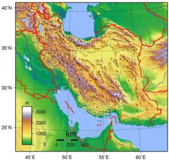
Fig. 1.Topography and Synoptic stations distribution over Iran.
suggest that statistically post-processed multi-model ensem-bles can outperform individual ensemble systems, even in cases in which one of the constituent systems is superior to the others. Beside the predictive PDF one can get a point or deterministic-style forecast by using just a weighted average of the individual forecasts in the ensemble.
Raftery et al. (2005) proposed and applied the BMA to surface temperature and mean sea level pressure forecasts of the University of Washington short-range ensemble with five members. They got calibrated and sharp predictive PDFs. This method has been used for post-processing the ensem-ble outputs for temperature, wind direction and precipitation in some other parts of the world with success. For example, Wilson et al. (2007) applied the BMA to calibrate surface temperature forecasts from the 16-member Canadian ensem-ble system. Assessment of the post-processed ensemensem-ble out-puts with around 40 days training period showed a good cal-ibration of the ensemble dispersion.
BMA was originally developed for weather quantities in which PDFs could be approximated by normal distributions, such as temperature and sea level pressure. Bao et al. (2010) extended and applied the BMA to 48-h forecasts of wind direction using von Mises densities as the component dis-tributions centered at the individually bias-corrected ensem-ble surface wind direction and could get consistent improve-ments in forecasts. Sloughter et al. (2007) used a mixture of a discrete component at zero and a gamma distribution as pre-dictive PDF for individual ensemble members and applied the BMA to daily 48-h forecasts of 24-h accumulated pre-cipitation in the North American Pacific Northwest in 2003– 2004 using the University of Washington mesoscale ensem-ble. They could get PDFs corresponding to probability of
precipitation forecasts that were much better calibrated com-pared to consensus voting of the ensemble members. The results of BMA were also better estimations of the probabil-ity of high-precipitation events than logistic regression on the cube root of the ensemble mean.
The present study aims at producing calibrated surface temperature forecasts at 299 meteorological stations scat-tered across Iran (Fig. 1) using a multi-model multi-analysis ensemble for the period from 15 December 2008 to the 11 June 2009. Predictive forecast PDFs’ performances are evaluated using reliability and ROC diagrams. Point or deterministic-style BMA forecasts are compared with de-terministic forecast of individual members using standard scores.
The paper is organized as follows: the BMA procedure is described briefly in Sect. 2, while the implementation details are presented in Sect. 3. Verification results are discussed in Sect. 4 and finally, conclusions and proposal for further works are drawn in Sect. 5.
2 Calibration method
Bayesian Model Averaging (BMA) was proposed by Raftery et al. (2005) as a statistical post-processing approach for combining different model forecasts and producing full pre-dictive PDFs from ensembles, subject to calibration and sharpness. In the following a brief description of the method is presented, but the reader is referred to Raftery et al. (2005) for full details. The BMA predictive PDF of the weather quantity to be forecast is a weighted average of PDFs de-fined around each individual bias-corrected ensemble mem-ber. The individual PDFs for the ensemble members need not to be Gaussian or even the same. In this study, as in Raftery et al. (2005), the weather quantity to be forecast,y, is temperature whose behavior can be estimated by a normal distribution. Hence a Gaussian distribution,hk(y|fk), is de-fined around each individual forecast,fk, conditional onfk being the best forecast in the ensemble. The BMA predictive PDF is then a conditional probability for a forecast quantity
ygivenKmodel forecastsf1, . . . ,fk, and is given by:
p(y|f1,...fk)=
XK
k=1wkgk(y|fk) (1) wherewkis the posterior probability of forecastkbeing the best one, and is based on forecastk’s relative performance over a training period. Thewk’s are nonnegative probabili-ties and their sum is equal to 1, that isPKk=1wk. Here K, the number of ensemble members, is equal to 7. gk(y|k)is a univariate normal PDF with mean fk=ak+bkfk, (bias-corrected forecast) that is a linear function of forecast fk, and standard deviationσ2assumed to be constant across en-semble members. This situation is denoted by:
Table 1.Ensemble members configuration.
Member Cumulus Planetary boundray layer Microphysic Long wave radiation Short wave radiation Surface layer Land surface Initial
name conditions
WRF1 Kain-Fritsch (new Eta) scheme
MRF scheme Kessler scheme RRTM scheme Dudhia scheme Monin-Obukhov scheme Noah land-surface Model GFS WRF2 Grell-Devenyiesemble scheme
MRF scheme Kessler scheme RRTM scheme Dudhia scheme Monin-Obukhov scheme Noah land-surface Model GFS WRF3 Betts-Miller-Janjic scheme
MRF scheme Kessler scheme RRTM scheme Dudhia scheme Monin-Obukhov scheme
Noah land-surface Model
GFS
WRF4 Kain-Fretsch Mellor-Yamada-Janjic Lin RRTM scheme Goddard Monin-Obukhov– Janic scheme
Noah GFS
WRF5 Grell-Devenyi ensem-ble
Mellor-Yamada-Janjic WSM3 RRTM scheme Dudhia scheme Eta similarity 5-layer thermal dif-fusion
GFS
MM5 Betts-Miller-Janjic scheme
Mellor-Yamada-Janjic Mixed phase CCM2 CCM2 Monin-Obukhov scheme
5-layer soil model GFS
HRM Mass flux (Tiedtke) Mellor-Yamada-Janjic Doms and Sch¨attler δ-2 stream radiation scheme Level-2 scheme and 7-layer soil model GME
Coefficientsak andbk in the mean of the individual PDFs vary with time and location and are estimated by a linear re-gression of observed temperature, y, on modelkforecasts,
fk, in the training period, for each time and location sepa-rately. This regression can be considered as a preliminary debiasing of the deterministic forecasts in the ensemble. The
Kweights or posterior probabilitieswk and varianceσ2are estimated using maximum likelihood (Fisher et al., 1922). For a fixed set of training data and underlying normal proba-bility model, the method of maximum likelihood selects val-ues of the model parameters that maximize the likelihood function, that is, the value of the parameter vector under which the observed data were most likely to have been ob-served. For both mathematical simplicity and numerical sta-bility, usually the log-likelihood function is used for maxi-mization rather the likelihood function itself. Usually, the maximum value of the log-likelihood function is evaluated using the expectation-maximization (EM) algorithm (Demp-ster et al., 1977; McLachlan and Krishnan, 1997). The BMA deterministic forecast also can be calculated by weighted av-eraging of theKdeterministic forecasts usingwkas weights, that is:
XK
k=1wk(akfk+bk) (3)
3 The ensemble system and data
Forecasts of the Weather Research and Forecasting (WRF: Skamarock et al., 2008) model with five different configu-rations, The fifth-generation Pennsylvania State University– National Center for Atmospheric Research Mesoscale Model (MM5: Dudhia, 1993; Grell et al., 1994) and High Resolu-tion Model (HRM: Majewski, 1991, Majewski and Schrodin, 1994) of the Deutscher Wetter Dienst (DWD) both with one configuration for 2-m temperature, 48-h in advance are used in this study to build a seven-member ensemble. The model settings are presented in Table 1. As seen in the table the main differences between different model setups
pertain to convective and boundary layer parameterization schemes. WRF and MM5 are used with non-hydrostatic op-tion whereas HRM is hydrostatic. The initial and boundary conditions come from the operational 12Z runs of the global forecasting system (GFS) of NCEP (National Center for En-vironmental Prediction) (Sela, 1980) for MM5 and WRF and of DWD’s global model (GME) for HRM models respec-tively. The integration period goes from 15 December 2008 to 11 June 2009.
The period of study includes spring and summer seasons. In the onset of spring, subtropical anticyclone migrates to northern latitudes and hence baroclinic mid-latitude systems are weakened over south and central part of Iran. During summer time the mid-latitude synoptic baroclinic systems enter Iran from west and north-west and influence the coun-try only in the north-west. The cold air associated with these systems, causes rapid temperature changes in the northern part of Iran. As we enter from spring to summer, the sub-tropical anticyclone becomes dominant over most part of the country and many places experience their maximum temper-ature during summer. In some places the tempertemper-ature ex-ceeds 50 and reaches even 55◦C. In the southern part of the country, there is an interaction between Iranian heat low and the Indian monsoon low that causes the convective systems to become dominant and play an important role in the tem-perature changes over these regions.
MM5 and WRF were run with two nested domains, with the larger domain covering the south-west middle east from 10◦ to 51◦ north and from 20◦ to 80◦east and the smaller domain covers Iran from 23◦ to 41◦north and from 42◦ to 65◦east. The spatial resolutions are 45 and 15-km for the coarser and finer domains, respectively. The inner domain in HRM considered here, covers from 25◦to 40◦north and from 43◦to 63◦east with spatial resolution of 14-km. Totally 1134 simulation have been performed and forecasts out to
Fig. 2. Comparison of training period length for surface tempera-ture: diagram of(a)MAE, RMSE,(b)CRPS, and(c)ME for from 10 to 65 days.
The data used in this study consist of 12Z observations of 2-m temperature at 299 irregularly spaced synoptic meteoro-logical stations scattered all over the country from 15 Decem-ber 2008 to the 11 June 2009 and corresponding 48-h fore-casts from the above mentioned seven members of the en-semble bi-linearly interpolated to the observation sites. The geographical distribution of the synoptic stations is presented in Fig. 1. UsingNdays as training period, the BMA predic-tive PDF, Eq. (1), and BMA deterministic forecast, Eq. (3), for the 2-m temperature were evaluated for each station site and the remaining days.
4 Training period
The sample of past days,N, used as training period, in esti-mating the unknown parameters (ak,bk,wk andσ) in Eq. (2) is a sliding training window, such that new coefficients are estimated for each day using the most recent N days as training period. In principle, length of the training period must be such that it does not lead to over-fitting.
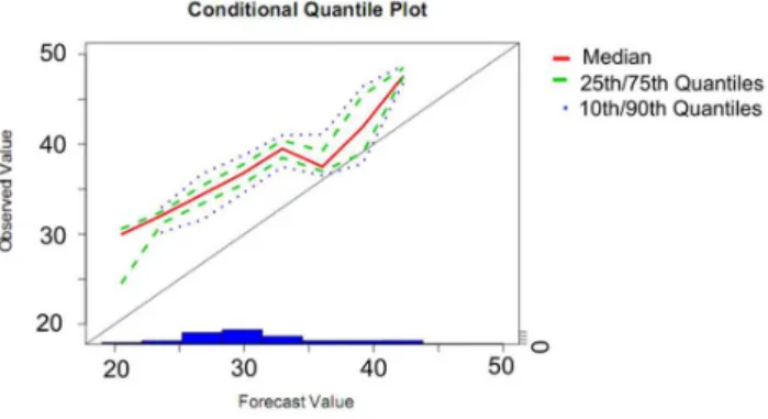
How-Fig. 3. Conditional Quantile Plot (CQP) diagram for MM5 2-m temperature forecasts.
ever, longer training periods increase statistical variability and shorter training periods make the forecast system to re-spond more quickly to changes in the model error patterns due to weather regime changes. It is clear that using short training periods have the advantage of data availability and ease of computations. A balance should be made in deter-mining the length of the training period. In this study, as in Raftery et al. (2005), some experiments were conducted with training period changing from 10 to 65-day. Figure 2 shows the mean absolute error (MAE), root mean squared er-ror (RMSE) and mean erer-ror (ME) of the BMA deterministic forecasts and the continuous rank probability score (CRPS) versus training days. Minimum errors can be seen on the figure around 20 and 40 days training period. But increas-ing the trainincreas-ing days beyond 40 does not change the results significantly and the error remains almost constant or even increases. So, a 40-day window was selected as the training period.
5 Results and discussion 5.1 Raw ensemble
Figure 3 presents an example of the conditional quantile plot (CQP) (Wilks, 2006) for 48-h temperature forecast of one member (member 6: MM5) in the ensemble for the period mentioned in Sect. 2. It is clear that deterministic forecasts, corresponding to the 7th ensemble member show a cold bias and thus a debiasing of the forecasts is needed. The CQPs related to other ensemble members (not shown here) show similar results, i.e. a cold bias.
Fig. 4.Rank histogram of the raw ensemble for 48-h surface tem-perature forecasts.
Fig. 5.Minimum Absolute Error (MAE) and maximum error for all ensemble members and calibrated BMA outputs.
Under-dispersion of the ensemble is reflected in the non-uniform shape of its rank histogram. As it is seen from the figure, the rank histogram for the raw ensemble is a sloped one, showing a consistent bias in the ensemble forecast. The ensemble members have under-forecast or cold bias, such that around 50 % of the times the observed temperature was greater than all the ensemble member values. This result is consistent with the results presented in Fig. 3. The under-dispersion for the raw ensemble has been reported in many other studies. The goal of post-processing is to correct for such known forecast errors, i.e. to construct a calibrated en-semble with statistical properties similar to the observations.
5.2 Deterministic BMA forecast
For comparing the deterministic BMA forecast (Eq. 3) with the deterministic forecast corresponding to the best member of the ensemble, the mean absolute error (MAE) and per-centage of successful forecasts (forecasts with less than 2◦C difference from the verifying observation) are considered. In terms of MAE, Fig. 5 shows that MAE of the deterministic forecasts of the seven members of the ensemble system are between 2.2 to 6.7◦C, while that of the BMA deterministic forecast is lower and around 2◦C.
Fig. 6.Histogram of percentage of acceptable forecast of raw data and BMA outputs for±2◦C error.
Table 2.Weights of two synoptic stations of Piranshahr and Noshahr in initialized at 12:00 UTC on 1 February and 1 May 2009, respectively.
HRM MM5 WRF5 WRF4 WRF3 WRF2 WRF1 Date Station
0.348 0.175 0.246 0.216 3.02×10⁻³ 7.1×10⁻⁶ 0.0112 20090401 Noshahr 0.20 0.170 0.399 0.212 0.0115 2.98×10⁻⁶ 6.8×10⁻³ 20090501 Piranshahr
Table 3.Performance scores for eight categories ranging from “equal to 0◦C” out to “above 30◦C” with 5◦C interval.
Freezing point 0 to 5 5 to 10 10 to 15 15 to 20 20 to 25 25 to 30 above 30
Brier Score (BS) 0.017 0.052 0.102 0.123 0.102 0.069 0.035 0.013
Brier score – baseline 0.024 0.076 0.158 0.188 0.162 0.124 0.063 0.027
Skill score 0.305 0.324 0.359 0.345 0.374 0.447 0.443 0.543
Reliability 0.002 0.002 0.001 0.000 0.002 0.001 0.002 0.003
Resolution 0.010 0.027 0.057 0.065 0.062 0.057 0.030 0.017
Uncertainty 0.024 0.076 0.158 0.188 0.162 0.124 0.063 0.027
Fig. 8.Probability Integral Transform (PIT) histogram of calibrated BMA outputs.
Percentage of the successful forecasts for seven members of the ensemble, shown in Fig. 6, ranged from 3.6 % to 56.5 % for the first and fifth members, respectively. This score for the BMA deterministic forecast is close to 62 % which is again better that those of all ensemble members. It is thus seen that the BMA deterministic forecast outperforms all other seven deterministic forecasts corresponding to the ensemble members.
5.3 Calibrated ensemble
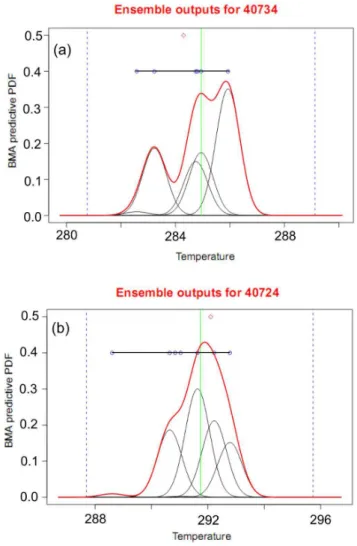
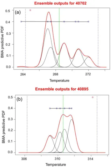
One main aim of the ensemble forecasting is to account for various uncertainties in the ensemble system for issuing probabilistic forecasts. Figure 7a and b shows two examples of the final predictive BMA for 48-h forecast of 2-m temper-ature valid at first February and first May 2009, along with
its seven normal PDF components issued for two synoptic stations of Piranshahr and Noshahr located in the west and north of the country. As is seen, the calibrated BMA PDF that is a weighted sum of its seven components, is a non-normal distribution. Table 2 shows the calculated weights given to each member of the ensemble. It is seen that for Noshahr, the weights in descending order are given to HRM, WRF5, WRF2 and MM5 members respectively, while for Piranshahr are given to WRF5, WRF4, HRM and MM5. As mentioned above, a higher weight given to a member means that member is more useful. But, as mentioned by Gneit-ing et al. (2005), low weight for a member does not mean necessarily a lower performance of that member. If there are colinearities between two (or more) ensemble members, then their informations are similar and one of them might be given low weight though this member alone might be skillful.
One important aim of applying the BMA technique is to obtain a well calibrated ensemble with reduced under-dispersion. The fact that the predictive PDFs are calibrated is reflected in the uniformity of the post-processed ensemble rank histogram for 48-h forecasts, presented in Fig. 8. As the figure shows, the BMA has been very successful in calibrat-ing the raw ensemble forecasts.
Fig. 9. Attribute diagrams for(a)raw ensemble and(b)BMA for “20 to 25◦C” interval. In this figure a horizontal “no resolution” line is drawn at the climatological frequency. A vertical line is also drawn for a forecasted probability at the observed frequency, a “per-fect reliability line” is also drawn with a slope of 1.
25◦C interval which indicates for most of probabilities raw ensemble has no skill. Attribute diagrams of BMA weighted mean for the same interval in Fig. 9b shows significant im-provement over the raw ensemble (Fig. 9a and b).
The ROC (Relative Operating Characteristic or Receiver Operating Characteristic) diagram is another discrimination-based graphical forecast verification display (Wilks, 2006). The ROC was first introduced into meteorology by Mason (1982), is a graphical plot of hits against false alarms, us-ing a set of increasus-ing probability thresholds. The area under the ROC curve is a measure of performance. An area equal to 1 implies perfect performance, while an area of 0.5 corre-sponds to random forecasts or to the climatological forecasts. Results from the calibrated ensemble for various threshold values, as those used for attribute diagrams, for 48-h temper-ature forecasts indicate that the ensemble exhibit good event discrimination (Fig. 10). It is seen that for warmer thresholds (greater than 20◦C) and freezing point, the ROC curve bows
Fig. 10.Relative operating characteristic (ROC) diagrams for eight temperature categories ranging from “equal to 0◦C” out to “above 30◦C” with 5◦C interval.
the most beyond the diagonal line and thus the ensemble for these thresholds shows more discriminating than others.
Figure 11 shows BMA predictive PDF for two extreme events one with minimum and another with maximum 2-m temperature. Minimum surface temperature during the study period happened on 2 January 2009 at Jolfa located in the north of Iran, while Nik-Shahr in the south-east of the coun-try experienced the maximum temperature record on 28 April 2009. In both cases, most of the ensemble members have not simulated the surface temperature; this is probably be-cause mesoscale models have difficulty in correctly forecast-ing extreme temperatures. BMA gave the highest weight to the member that had better surface temperature prediction, WRF5 (Fig. 11a), while for other case, minimum tempera-ture event, the best forecast of surface temperatempera-ture was given by MM5 and WRF5, for this case, MM5 underestimated the temperature and was assigned the least weight while WRF5 obtained the highest weight.
6 Conclusion
This paper describes the results of 48-h probabilistic surface temperature forecasts over Iran for the period of 15 Decem-ber 2008 to 11 June 2009 using Bayesian Model Averaging for calibration of the ensemble outputs. The ensemble sys-tem consists of the WRF model with five different configu-rations, MM5 and HRM both with one configuration. The initial and boundary conditions come from the operational 12Z runs of GFS for MM5 and WRF, and GME for HRM models respectively.
Fig. 11. Same as Fig. 7, but for(a)Jolfa on 2 January 2009 and
(b)Nik-Shahr on 28 April 2009.
Overall results showed that the BMA technique is al-most successful at removing al-most, but not all of the under-dispersion exhibited by the raw ensemble and thus attaining higher reliability in the probabilistic forecasts that could be used in an operational framework. Using the weighted en-semble mean forecast as a deterministic forecast it was found that the deterministic-style BMA forecasts performed almost always better than the best member’s deterministic forecast in the ensemble.
Acknowledgements. Financial support for this research is gratefully acknowledged from Khuzestan Water & Power Autority Co., Iran. The authors also appreciate the useful discussions and suggestions from D. Parhizkar from Atmospheric Science and Meteorological Research Center (ASMERC) and M. Khodadi from I. R. of Iran Meteorological Organization (IRIMO).
Topical Editor P. Drobinski thanks C. Santos and another anony-mous referee for their help in evaluating this paper.
References
Bao, L., Gneiting, T., Grimit, E. P., Guttorp, P., and Raftery, A. E.: Bias Correction and Bayesian Model Averaging for Ensemble Forecasts of Surface Wind Direction, Mon. Weather Rev., 138, 1811–1821, 2010.
Dempster, A., Laird, N., and Rubin, D.: Maximum likelihood from incomplete data via the EM algorithm, J. R. Stat. Soc., Series B, 39(1), 1–38, 1977.
Dudhia, J.: A nonhydrostatic version of the Penn State/NCAR mesoscale model: Validation tests and the simulation of an At-lantic cyclone and cold front, Mon. Weather Rev., 121, 1493– 1513, 1993.
Eckel, F. A. and Mass, C. F.: Aspects of effective mesoscale, short-range ensemble forecasting, Wea. Forecasting, 20, 328– 350, 2005.
Fisher, R. A., Thornton, H. G., and Mackenzie, W. A.: The accu-racy of the plating method of estimating the density of bacterial populations, CP22 in Bennett 1971, vol. 1., Annals of Applied Biology, 9, 325–359, 1922.
Gneiting, T., Raftery, A. E., Westveld, A. H., and Goldman, T.: Cal-ibrated probabilistic forecasting using ensemble Model Output Statistics and minimum CRPS estimation, Mon. Weather Rev., 133, 1098–1118, 2005.
Grell, G. A., Dudhia, J., and Stauffer, D. R.: A description of the fifth-generation Penn State/NCAR mesoscale model (MM5), NCAR Tech. NoteTN-398+STR, 122 pp., 1994.
Grimit, E. and Mass, C.: Initial results of a mesoscale short-range ensemble forecasting system over the Pacific Northwest, Weather Forecast., 17, 192–205, 2002.
Hamill, T. M.: Interpretation of rank histograms for verifying en-semble forecasts, Mon. Weather Rev., 129, 550–560, 2001. Hamill, T. M. and Colucci, S. J.: Verification of Eta–RSM
short-range ensemble forecasts, Mon. Weather Rev., 125, 1312–1327, 1997.
Hamill, T. M. and Colucci, S. J.: Evaluation of Eta–RSM ensem-ble probabilistic precipitation forecasts, Mon. Weather Rev., 126, 711–724, 1998.
Hersbach, H.: Decomposition of the Continuous Ranked Probabil-ity Score for Ensemble Prediction Systems, Weather Forecast., 15, 559–570, 2000.
Hou, D., Kalnay, E., and Droegemeier, K. K.: Objective verification of the SAMEX’98 ensemble forecasts, Mon. Weather Rev., 129, 73–91, 2001.
Houtekamer, P. L. and Derome, J.: The RPN ensemble predic-tionsystem. Proceedings, ECMWF Seminar on Predictability. Vol. II. ECMWF, 121–146, available from ECMWF, Shinfield Park,Reading, Berkshire RG2 9AX, United Kingdom, 1996. Majewski, D.: The Europa-Model of the DWD, ECMWF
Semi-nar on numerical methods in Atmospheric Science, 2, 147–191, 1991.
Majewski, D. and Schrodin, R.: Short description of Europa-Model (EM) and Deutschland Model (DM) of the DVD, Q. Bull, 1994. Mason, I. B.: A model for assessment of weather forecasts, Austral.
Met. Mag., 30, 291–303, 1982.
McLachlan, G. and Krishnan, T.: The EM algorithm and extensions. Wiley series in probability and statistics, John Wiley & Sons, 1997.
val-idation, Q. J. Roy. Meteorol. Soc., 122, 73–119, 1996.
Raftery, A. E., Gneiting, T., Balabdaoui, F., and Polakowski, M.: Using Bayesian model averaging to calibrate forecast ensembles, Mon. Weather Rev., 133, 1155–1174, 2005.
Roulston, M. S. and Smith, L. A.: Combining dynamical and statis-tical ensembles, Tellus, 55A, 16–30, 2003.
Sela, J. G.: Spectral Modeling at the National Meteorological Cen-ter, Mon. Weather Rev., 108, 1279–1292, 1980.
Skamarock, W. C., Klemp, J. B., Dudhia, J., Gill, D., Barker, D., Wang, W., and Powers, J. G.: A description of the Advanced Re-search WRF Version 3, NCAR Tech. Note NCAR/TN-475+STR, 2008.
Sloughter, J. M., Raftery, A. E., Gneiting, T., and Fraley, C.: Prob-abilistic quantitative precipitation forecasting using Bayesian model averaging, Mon. Weather Rev., 135, 3209–3220, 2007. Stensrud, D. J. and Yussouf, N.: Short-range ensemble predictions
of 2-m temperature and dewpoint temperature over New Eng-landm Mon. Weather Rev., 131, 2510–2524, 2003.
Stensrud, D. J., Brooks, H. E., Du, J., Tracton, M. S., and Rogers, E.: Using ensembles for short-range forecasting, Mon. Weather Rev., 127, 433–446, 1999.
Toth, Z. and Kalnay, E.: Ensemble forecasting at NMC: Thegener-ation of perturbThegener-ations, B. Am. Meteorol. Soc., 74, 2317–2330, 1993.
Wandishin, M. S., Mullen, S. L., Stensrud, D. J., and Brooks, H. E.: Evaluation of a short-range multimodel ensemble system, Mon. Weather Rev., 129, 729–747, 2001.
Wang, X. and Bishop, C. H.: Improvement of ensemble reliability with a new dressing kernel, Q. J. Roy. Meteorol. Soc., 131, 965– 986, 2005.
Wilks, D. S.: Statistical Methods in the Atmospheric Sciences, 2nd Edition, Academic Press, 627 pp., 2006.