Submitted9 December 2015 Accepted 2 February 2016 Published29 February 2016 Corresponding author Benjamin H. Letcher, [email protected]
Academic editor Jack Stanford
Additional Information and Declarations can be found on page 21
DOI10.7717/peerj.1727 Distributed under
Creative Commons Public Domain Dedication
OPEN ACCESS
A hierarchical model of daily stream
temperature using air-water temperature
synchronization, autocorrelation, and
time lags
Benjamin H. Letcher1, Daniel J. Hocking1, Kyle O’Neil1, Andrew R. Whiteley2,
Keith H. Nislow3and Matthew J. O’Donnell1
1S.O. Conte Anadromous Fish Research Center, US Geological Survey/Leetown Science Center, Turners Falls,
USA
2Department of Environmental Conservation, University of Massachusetts, Amherst, USA 3Northern Research Station, USDA Forest Service, University of Massachusetts, Amherst, MA, USA
ABSTRACT
Water temperature is a primary driver of stream ecosystems and commonly forms the basis of stream classifications. Robust models of stream temperature are critical as the climate changes, but estimating daily stream temperature poses several important challenges. We developed a statistical model that accounts for many challenges that can make stream temperature estimation difficult. Our model identifies the yearly period when air and water temperature are synchronized, accommodates hysteresis, incorporates time lags, deals with missing data and autocorrelation and can include
external drivers. In a small stream network, the model performed well (RMSE=
0.59◦C), identified a clear warming trend (0.63 ◦C decade−1) and a widening of the
synchronized period (29 d decade−1). We also carefully evaluated how missing data
influenced predictions. Missing data within a year had a small effect on performance
(∼0.05% average drop in RMSE with 10% fewer days with data). Missing all data for a
year decreased performance (∼0.6 ◦C jump in RMSE), but this decrease was moderated
when data were available from other streams in the network.
SubjectsConservation Biology, Ecology, Environmental Sciences
Keywords Stream temperature, Ecology, Air temperature, Statistical model, Climate change
INTRODUCTION
Accurate stream temperature predictions are increasingly important as human impacts
on streams and on the climate accelerate stream temperature change (Kaushal et al.,
2010;Rice & Jastram, 2015). Human activities influence stream temperatures directly
via increased water withdrawals, altered channel engineering and dam operation (Poole
& Berman, 2001) and indirectly by altering landscape features (e.g., riparian cover) and by affecting air temperatures at broad spatial scales via climate change (Hayhoe et al., 2007;Huntington et al., 2009). Understanding how stream temperatures are changing over time and space and the ability to forecast future temperatures are important because
stream temperatures directly influence stream ecosystems (Quinn et al., 1994;Wenger et
for managing streams and their watersheds (e.g.,Beauchene et al., 2014). Altered stream temperatures are likely to have profound effects on the abundance and distribution of stream biota (Isaak & Rieman, 2013;Eby et al., 2014), especially coldwater, ectothermic species because many physiological and demographic rates are temperature-dependent (Fry, 1971;Elliott & Elliott, 2010;Letcher et al., 2015).
The general importance of stream temperature has prompted the development of a number of models for stream temperature (e.g.,Mohseni, Stefan & Erickson, 1998;
Caissie, El-Jabi & Satish, 2001;Hague & Patterson, 2014;Sun et al., 2014;Li et al., 2014). Stream temperature models vary along several important gradients, including model type (physical-statistical), temporal resolution (daily-yearly) and spatial resolution (local-broad spatial coverage). As with all models of complex systems, tradeoffs among these gradients usually limit models to highly-detailed, local models (Brown, 1969;Kim & Chapra, 1997;Younus, Hondzo & Engel, 2000) or simple, general models (e.g.,Crisp & Howson, 1982). The detailed, local models typically produce good accuracy (RMSE
∼1.0 ◦C) but may not predict temperatures well outside of the local area, while the
simple models generate moderate to poor accuracy (RMSE∼1.5–3.0 ◦C) across a broad
spatial range. Models that aggregate over longer time intervals generally perform better (Stefan & Preud’homme, 1993;Pilgrim, Fang & Stefan, 1998;Webb, Clack & Walling, 2003;
Morrill, Bales & Conklin, 2005), but even hourly models can perform well (Kanno, Vokoun & Letcher, 2014). A careful consideration of six key temperature modeling issues may provide the basis for the development of effective daily stream temperature models of medium complexity.
First, the relationship between air temperature and stream temperature is non-linear at high and low air temperatures (Mohseni, Stefan & Erickson, 1998), but for different reasons. At high air temperatures, evaporative cooling slows warming of stream water, while at low air temperatures, air temperatures can dip well below the water temperature freezing limit (Caissie, 2006;Webb et al., 2008). Air and water temperatures are no longer
synchronized when air temperatures are near and below 0 ◦C, which can generate a poor
relationship between air and stream temperatures and heterogeneity of variance across temperatures. Many simple statistical models use a non-linear model to describe the relationship between air and stream temperature (Mohseni, Stefan & Erickson, 1998;Webb, Clack & Walling, 2003;Kanno, Vokoun & Letcher, 2013). Others use a linear model and limit analysis to the summer (Hilderbrand, Kashiwagi & Prochaska, 2014) or to the ice-free period of the year (Stefan & Preud’homme, 1993;Erickson & Stefan, 2000), in an attempt to avoid the non-linear portions of the air-water temperature relationship. Time series (Caissie, El-Jabi & St-Hilaire, 1998;Caissie, El-Jabi & Satish, 2001;Benyahya et al., 2007) or non-parametric models (Benyahya et al., 2008;Li et al., 2014) of stream temperature trends over time that include air temperature as a predictor as well as local, physical models (e.g.,Sinokrot & Stefan, 1993) can accommodate the non-linearity.
of cool snow melt or rain water in the spring (Lisi et al., 2015) which depresses spring stream temperature/air temperature relationships relative to fall stream temperature/air temperature relationships (Webb & Nobilis, 1997).Mohseni, Stefan & Erickson (1998)
observed that 43% of their study streams exhibited hysteresis; they addressed hysteresis by fitting separate non-linear curves to the rising and falling seasonal temperatures. Time series models with non-symmetric seasonal functions account for hysteresis by default (e.g.,Li et al., 2014).
Third, due to thermal inertia, stream temperature does not respond instantaneously to changes in air temperature. Including lags in air temperature effects can improve estimates for models with short time scales (Benyahya et al., 2008;Webb, Stewardson & Koster, 2010). The effects of time lags increase with stream depth (Stefan & Preud’homme, 1993) and stream flow (Smith & Lavis, 1975;Webb, Clack & Walling, 2003). Time lags are a key component of time series modeling (Shumway & Stoffer, 2006).
Fourth, while the amount of stream temperature data available worldwide is increasing very rapidly (Webb et al., 2008), many sites have incomplete data. Very few study regions have a complete matrix of sample sites and years: data may be missing for an entire year at a site or may be incomplete within a year. Incomplete within-year data will have variable effects on estimation depending on the extent and timing of the missing data. Effects of missing data will also depend on model type. For simple linear models, within-year missing data may not have a large effect on estimation because of the linear relationship between stream and air temperature. For non-linear models, missing data could have dramatic effects on estimation as missing data fail to ‘anchor’ the curve. Other modeling
approaches, such as time series models , machine learning models (DeWeber & Wagner,
2014), and models with varying coefficients (Li et al., 2014) may be less sensitive to missing data. In general, hierarchical models with random effects across space (sites, stream networks or regions) and time (months, seasons, or years) can accommodate missing data as they ‘borrow information’ across units (Wagner, Hayes & Bremigan, 2006;
Gelman & Hill, 2006).
Fifth, spatial and temporal autocorrelation can cause estimation problems (Caissie, 2006;Benyahya et al., 2007;Hague & Patterson, 2014). Autocorrelation occurs when data points in space or time are not independent, i.e., close points are similar or dissimilar to each other simply because they are close. For example, downstream temperatures can be similar to upstream temperatures because water flows downstream or today’s temperature can be similar to yesterday’s temperature due to the combination of high heat capacity of water, low density and heat transfer from air, and conduction of heat from surrounding environment (i.e., thermal inertia) (Caissie, El-Jabi & St-Hilaire, 1998;
Isaak et al., 2014). This is a very common issue in estimation and a variety of time series
models can accommodate temporal autocorrelation (Shumway & Stoffer, 2006) and some
newer approaches are now available to deal with spatial autocorrelation (Peterson & Ver Hoef, 2010;Rushworth et al., 2015).
Finally, air temperature is not the only important predictor of stream temperature (Webb, 1996;Caissie, 2006). Many regression-based models have evaluated effects of
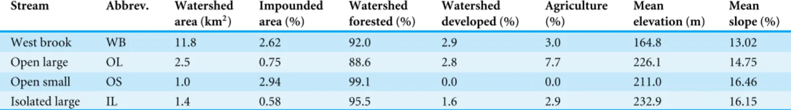
Table 1 Landscape variables for the four study streams (Fig. 1).
Stream Abbrev. Watershed area (km2)
Impounded area (%) Watershed forested (%) Watershed developed (%) Agriculture (%) Mean elevation (m) Mean slope (%)
West brook WB 11.8 2.62 92.0 2.9 3.0 164.8 13.02
Open large OL 2.5 0.75 88.6 2.8 7.7 226.1 14.75
Open small OS 1.0 2.94 99.1 0.0 0.0 211.0 16.46
Isolated large IL 1.4 0.58 95.5 1.6 2.9 232.9 16.15
Isaak & Hubert, 2001;Hill, Hawkins & Carlisle, 2013). Important landscape drivers typically include topography, riparian cover, impervious surface, and stream depth (Poole & Berman, 2001) and environmental drivers often include stream flow, snow melt, groundwater input, and humidity (Taylor et al., 2013;Lisi et al., 2015;Snyder, Hitt & Young, 2015). It is generally straightforward to incorporate external drivers beyond air temperature into most classes of stream temperature models (Hague & Patterson, 2014).
Here, we develop a model for mean daily stream temperature that improves accuracy of statistical models by addressing most of the issues listed above. To avoid fitting a relationship between stream and air temperature when there is none (e.g., winter), we develop a metric that limits estimation to the days of the year that daily stream temper-ature and daily air tempertemper-ature are synchronized (roughly spring to fall). This metric is flexible among years and sites. To address hysteresis, we estimate a non-symmetrical trend across the synchronized days with a hierarchical structure to accommodate missing data. We also add an autoregressive term to the model to deal with temporal autocorrelation and we estimate spatial covariance to accommodate spatial autocorrelation. Because data presented here are spatially constrained to four sites in a small network, we do not include landscape variables in the model. The two environmental drivers in the model are air temperature and stream flow. In addition to presenting the model, we analyze trends in estimates over time and conduct a detailed missing observations analysis.
METHODS
Study area
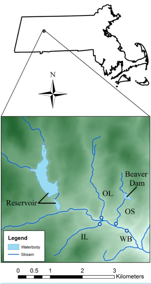
The study site was located in western Massachusetts, USA (42◦25′N; 72◦39′W,Fig. 1)
and consisted of a third-order mainstem (West Brook, WB) and three second-order tributaries (Open large, OL; Open small, OS; Isolated large, IL) (Fig. 1andTable 1). A dense canopy of mixed hardwood with some hemlocks provides cover throughout the
watershed. Watershed area above our study area is 11.8 km2and landuse in the area is
limited residential with some farming. The study is in an area of low to moderate relief,
with altitude ranging from to 100 m to 250 m (Fig. 1). Average stream width of the WB
is 4.5 m and is between 1–3 m for the tributaries. Water is stored in two of the streams; a drinking water reservoir is upstream of the WB, and a large beaver dam complex is above OS (Fig. 1). OL and IL were free-flowing during the course of the study.
We deployed temperature loggers (±0.1 C; Optic StowAway and Hobo Pro V2, Onset
Computer Corporation, Pocasset, MA, USA, and±0.05 C; Barologger, Solinst Canada
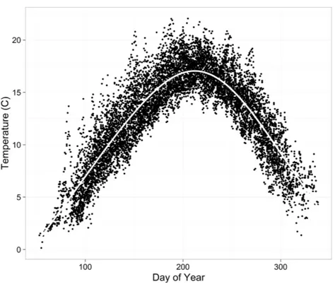
Figure 2 Water temperature data (daily means) from all sites and years overlain by a spline (white line).
Stream temperature data are available athttp://db.ecosheds.org. All loggers recorded data every two hours throughout the year. The logger in the WB was deployed 1998–2013 and the loggers in the tributaries were out from 2002 to 2013. We do not have continuous
air temperature measurements from 2002 to 2013 (Table 1), so we used mean daily air
temperature estimates for our study area from Daymet (http://daymet.ornl.gov/). For
the years that we do have West Brook air temperature data (2008–2013), the relationship between West Brook and Daymet air temperatures was strong (p-value < 10−16,r2=
0.91), suggesting that Daymet air temperatures are a good data source for the study site.
Stream flow was estimated using a flow extension model (Nielsen, 1999) based on data
from a nearby (∼10 km) USGS stream gage (Mill River, Northampton, MA, USA). See
Xu, Letcher & Nislow (2010)for details.
Statistical analysis Descriptive statistics
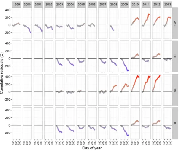
As a coarse comparison of daily water temperatures, we calculated correlations among sites. We also explored patterns in water temperature over time and among sites by
comparing cumulative residuals from a spline fit to all the data (function gam() inR,
Fig. 2). We calculated residuals for each water temperature data point and then developed empirical cumulative curves over days of the year for each year and site combination.
Breakpoints
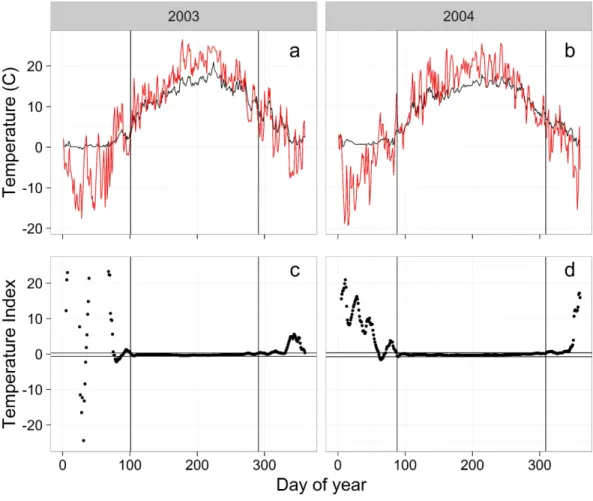
Figure 3 Examples of raw air (red) and water (black) temperatures from the WB (A, B) and the tem-perature index (C, D) used to calculate the temtem-perature breakpoints (vertical lines).Horizontal lines in (C) and (D) are the 99% confidence intervals of the temperature index for day of year 125–275. Vertical axes on (C) and (D) are truncated to−20–20.
lower water temperatures in the winter are bounded near 0 ◦C while air temperatures
are not. This means that water and air temperatures can become decoupled when air temperatures are cold resulting in only a weak relationship, at best, between water and air temperature. In contrast, as air temperatures warm in the spring and before they get
too cold in the autumn, daily water and air temperatures can be synchronized (Figs. 3A
and3B), suggesting the possibility of a strong relationship between daily water and air temperature during the synchronized portion of each year.
The key to the approach is identifying a breakpoint in the spring when daily water and daily air temperature become synchronized and a breakpoint in the autumn when daily temperatures become desynchronized. To identify the synchronization breakpoints
we calculated a simple index (waterT−airT)/waterT (waterT > 0), where waterT was
mean daily water temperature and airT was mean daily air temperature (Fig. 3). This
temperature index (tempIndex) approaches 0 when water and air temperature are
similar and is very different from 0 when temperatures diverge (Figs. 3Cand3D). While
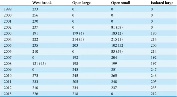
Table 2 Number of synchronized days with stream temperature data for each combination of year and site.Numbers in parentheses represent the percentage of days with missing data within the synchronized period.
West brook Open large Open small Isolated large
1999 233 0 0 0
2000 256 0 0 0
2001 230 0 0 0
2002 237 0 81 (58) 0
2003 191 179 (4) 183 (2) 180
2004 222 214 (3) 215 (1) 214
2005 235 203 102 (52) 200
2006 210 0 83 (59) 214
2007 0 192 204 192
2008 121 (45) 198 199 197
2009 0 243 251 247
2010 273 245 265 246
2011 233 205 248 205
2012 210 234 237 235
2013 226 218 0 212
providing the opportunity to identify the beginning and end (breakpoints) of the flat period.
To identify the spring and autumn breakpoints, we used a runs analysis that deter-mined the first (spring) and last (autumn) day of the year that the tempIndex was con-sistently within the flat period (Figs. 3Cand3D). We established the range of tempIndex values that comprised the flat period by calculating the 99.9% confidence interval (CI) for tempIndex using the middle 150 days of the year (late April to mid-September). The middle 150 days of the year were always within the flat period based on visual observation of tempIndex plots. Separate CI values were calculated for each year and stream. For the breakpoint estimation, we used a moving average for tempIndex with a centered 10-day window to help stabilize tempIndex values near the breakpoints. Temperatures were considered synchronized when 10 consecutive days of the moving average fell within the 99.9% CI. Beginning on day 1 and moving towards day 150, the first time 10 consecutive days were synchronized was used as the spring breakpoint and we moved from the end of the year to day 150 to establish the fall breakpoint. Numbers of days in the synchronized
period for each stream and year are shown inTable 2.
We evaluated trends in fall and spring breakpoints by running three linear models with
breakpoint day of the year as the dependent variable and year alone or year+stream
or year * stream as independent variables. We estimated AIC to determine the most parsimonious model.
Water temperature model description
linear autoregressive model with a cubic trend across days within a year and covariation among sites. We fit the model using a Bayesian approach.
Observed water temperature (ts,d,y) for each site (s;s1=WB,s2=OL,s3=OS,s4=IL),
day of year (d) and year (y) was assumed to derive from a normal distribution with mean
µs,d,y and standard deviationsd(residual model error):
ts,d,y∼N(µs,d,y,sd). (1)
We used a non-informative uniform prior [0, 10] forsd. We modeled the mean with a
linear trend (ωs,d,y) adjusted by an AR(1) autoregressive coefficient (δs) on the residual
error from the previous day:
µs,d,y=ωs,d,y+δs(ts,d−1,y−ωs,d−1,y). (2)
We placed a hierarchical structure onδs:
δs∼N(µδs,sdδ)T(−1,1) (3)
where site-specificδswere drawn from a truncated normal distribution with mean
µδsand standard deviationsdδ. Values forδswere truncated to keep them within the
admissible range for a correlation. Priors for the mean and standard deviation were non-informative;µδs∼U(−1,1), andsdδ∼U(0,2) (an upper limit of 2 forsdδis non-informative for the truncated data).
When observed temperature data were not available for the previous day (beginning of a series or following a break in the series) we modeled the mean without the autoregres-sive component:
µs,d,y=ωs,d,y. (4)
We modeled the linear component with a combination of fixed and random effects:
ωs,d,y=α+β1Ts,d,y+β2Ts,d−1,y+β3Ts,d−2,y+β4Fs,d,y+β5Ts,d,y·Fs,d,y+β6:8s
+β9:11s·Ts,d,y+Yy (5)
whereαis the overall intercept, theβare the coefficients for the fixed effects (T is mean daily air temperature,F is mean daily stream flow,sis site) andYy represents
random effects among years. Priors for theβ1:11were independent and non-informative,
N(0,100).
Yyrepresented random effect temporal trends (cubic) across years where:
Yy=αy+β12,yDs,y,d+β13,yD2s,y,d+β14,yD3s,y,d. (6)
For convenience, this equation can be written in matrix notation as
whereX is a data matrix withlcolumns (l=4; the number of year-level predictors) with
the first column a vector of 1’s for the intercept and By is they×lmatrix of year-level
regression coefficients. Priors for the mean were non-informative, with
By∼MVN(Ml,6) (8)
whereMl=(µα,µβ12,µβ13,µβ14) is a vector of lengthl, representing the mean of the
distribution of intercept and slopes. Thel×lcovariance matrix is represented by6where
the variance of each regression coefficient is on the diagonal and the covariance on the
off-diagonals. The hyperprior for the means were non-informative withµα,=0 and
µβ12,µβ13,µβ14∼N(0,100). Standard deviation priors were also non-informative and
were drawn from an inv-Wishart distribution:
6∼inv−wish(diag(l)l+1). (9)
Parameter estimation
We used the program JAGS (http://mcmc-jags.sourceforge.net) to code the model and to
draw posterior samples of the parameters (see Supplemental Information for JAGS code). We called JAGS from R (3.1.2) using the package ‘rjags’ (V 3-14). We ran three chains with 1,000 burn-in and 2,500 evaluation iterations. Chains were thinned to keep every fifth iteration. We checked convergence using the ‘potential scale reduction factor’ (Brooks & Gelman, 1998) from the ‘coda’ package in R (Plummer et al., 2006) and also assessed chains visually.
Model assessment
Goodness of fit and prediction
We assessed goodness of fit in two ways. First, we compared observed and predicted values for the complete dataset. Second, we ran a series of cross validation tests where we randomly left out a portion of the water temperature data, estimated parameters with the remaining (training) data and compared predictions of the left out (testing) data to original values. This involved leave-p-out cross-validation where we randomly left out a proportion (p) of the data, wherep=0, 0.05, 0.1, 0.2, 0.3, 0.4, 0.5, 0.6, 0.7, 0.8. We ran
10 replicates for each value ofp. For each condition, we calculated the root mean square
error (RMSE) of the residuals for the training and the test data sets.
Missing data
We also ran a series of tests to ask how the quantity, timing, and location of missing data influenced model performance (estimation and prediction). These tests can be used to help understand performance and to help design monitoring strategies. This set of analyses differed from the leave-p-out cross-validation (above) because data were not left out randomly. Rather, consecutive days of data were left out, either within a year or across streams, reflecting the character of missing field data.
complete data and then conducted nine sets of runs where we left out data 15·d days from
the beginning and 15·ddays from the end of each time series (whered=1–9), generating
shorter time series by 30 days for each scenario.
When: We assessed how changing the timing of missing data affected predictions by shifting the window of available data from the beginning to the end of the synchronized period. To do this, we left out data for all but 30 consecutive days at a time for 13 non-overlapping scenarios with scenario one starting at day of year 70 and scenario 13 starting at day of year 310.
Where: To evaluate how well the model predicted stream temperatures when data were missing from one or more streams, we ran the above analyses leaving out data yearly from all streams or just the West Brook. For years with data just from the West Brook (1999–2002), we removed all data a year at a time. For years with data from the tributaries and the West Brook (2003–2013), we either removed all the data for each year (all four streams) or just the data from the West Brook for each year. Removing all the data for a given year tests how well the model predictions work when there are no data for the year (but there are data for other years), while removing data for just the West Brook tests how well predictions work when data are missing for a stream (but there are data for other streams and years).
For all tests, we compared RMSE of the residuals for the test (left out) data to the RMSE of the residuals of the full training set (base case).
RESULTS
Descriptive statistics
Evaluation of the descriptive statistics suggested that water temperatures were similar for OL and IL and for WB and OS and that the streams appear to be warming over the duration of the study. Correlations of daily water temperatures among the four sites were all between 0.96 and 0.97, except for the correlation between OL and IL (0.99). Patterns in the cumulative water temperature residuals were generally similar for WB and OS, with cooler years in the beginning of the time series and warmer years later (Fig. 4). OS demonstrated the warmest temperatures, especially in 2010–2012. Patterns were remarkably similar between OL and IL, also demonstrating generally cooler temperatures earlier in the data time series (Fig. 4). Monthly distributions of water temperature were highly variable across years and streams (Fig. S1).
Parameter estimation
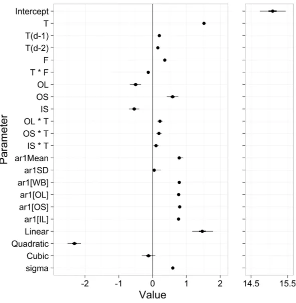
Potential scale reduction factor (R-hat) values for all parameters were less than 1.01, indicating good convergence (Brooks & Gelman, 1998). Parameter estimates gave an overall mean of 15.1, with strong air temperature effects (1.52 unlagged, 0.20 lagged 1 day, 0.15 lagged 2 days), a positive effect of stream flow (0.36), and strong site differences (OL
= −0.50, OS=0.59, IL= −0.54) (Fig. 5andTable S1). The autoregressive mean equaled
0.79 and there was little variation in the autoregressive terms among sites (Fig. 5). The
Figure 4 Cumulative residuals from the spline inFig. 2for each site and year combination.Curves on or near the horizontal line indicate ‘typical’ years whereas curves above the line indicate warm years and below the line indicate cool years.
Table 3 Root mean square error (RMSE,◦C) for various scenarios described in the text.The scenarios
involved a training dataset and a test dataset (data left out).
Scenario RMSE train Test streams RMSE test RMSE difference
All data 0.59±0.09 – – –
30% data randomly left out 0.69±0.003 All 0.86±0.010 0.17 For each year, West Brook left out 0.59±0.09 West brook 1.07±0.26 0.48 For each year, all streams left out 0.59±0.09 All 1.16±0.35 0.57
Model assessment: goodness of fit and prediction
Using the full dataset, predicted values were very similar to observed values (Fig. S2). The slope of the relationship was 0.99 (s.e.=0.0064) with an intercept of 0.15 (s.e.=0.089) and anR2of 0.98. Overall RMSE was 0.59±0.09 (Table 3). For the cross-validation tests
where we randomly left out 30% of the data, the RMSE increased to 0.69±0.003 for the
training data and to 0.86±0.010 for the test data (Table 3).
Figure 5 Parameter estimates from the stream temperature model.‘T’ stands for temperature, ‘F’ stands for flow, and OL, OS, IL are streams. The first 12 rows represent theβxinEq. (5). ‘ar1[x]’ are theδx
fromEq. (3), and the ‘Linear’, ‘Quadratic’ and Cubic’ parameters are theµYxfromEq. (7). ‘sigma’ is the residual standard deviation fromEq. (1).
proportion of data left out (r2=0.98;Fig. S3). RMSE for the training data set was largely
insensitive to the proportion of data left out and had a mean value of 0.86 (s.d.=0.016,
Fig. S3).
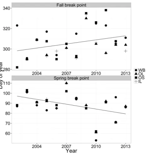
Break point trends
Break points appear to be getting later in the year in the fall and earlier in the year in the spring (Fig. 6). In the fall,1AIC values for the linear models were all within two
so we selected the simplest model (year only). In the spring, the1AIC value for the
Figure 6 Fall and spring breakpoints across years for the four streams.
year explained only 10% (fall) or 19% (spring) of the variation in the relationship. The parameter estimates indicated that breakpoints are 16 days earlier in the spring and 13 days later per decade in the fall, generating an estimated widening of the breakpoint window of 29 days per decade.
Trends in cubic functions
Predicted mean water temperatures based on the cubic function (Eq. (7)) varied among
years (Fig. S4), mirroring the general trend in the raw data (Fig. 2). Yearly maximum
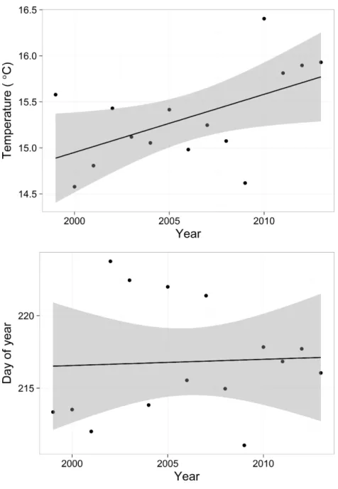
water temperature (white dots inFig. S4) increased over the course of the study (F=5.34, df =1,13,p-value=0.037,R2=0.24), with an estimated decadal increase of 0.63 ◦C (Fig. 7, above). In contrast, the day of year of the temperature maximum did not change over the course of the study (F=0.030,df =1,13,p-value=0.86) (Fig. 7, below).
Missing data: quantity
Figure 7 Predicted maximum temperature for each year (yaxis value of dot inFig. S4) and predicted
day of the maximum temperature (xaxis value of dot inFig. S4). Shadows represent 95% confidence
bands.
Missing data: when
The timing of data availability had a threshold effect on RMSE, with relatively high and variable RMSE before day 160 and consistent lower RMSE after day 160 (triangles in
Fig. 9).
Missing data: where
Compared to the base case (all data included), leaving data out of the estimation one year
at a time resulted in a mean increase in RMSE of 0.48 ◦C when just the WB data were left
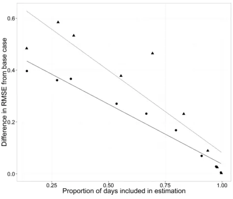
Figure 8 Root mean square error (RMSE) difference from the base case (all data included) for the WB for the cross-validation analyses changing the proportion of days included in estimation.Estimation data included either no data from any of the streams for each year (triangles, dashed line) or data from the three other streams but no data for the WB for each year (circles, solid line).
As the amount of data was increased on either side of the median date, RMSE increased less from the base case when data were available from the other three streams than when data were not available for any of the streams. The slope of the relationship between the proportion of days included in the training data and the difference in mean RMSE was
−0.46 when just the WB data were left out and the slope was−0.63 (s.e.=0.20) when data
from all streams were left out (Fig. 8). The slopes suggest either a 0.046 or a 0.063 decrease in RMSE with a 10% increase in days included in the estimation.
When data were available for only 30 days, but the 30-day window of availability varied across the year, the presence of data from the other streams eliminated the variability in
RMSE across scenarios (compare circles to triangles inFig. 9). The resulting increase in
RMSE was about 0.38 across 30-day window scenarios when data were present from other streams.
DISCUSSION
We present a statistical model that accounts for many issues that can make stream temperature estimation difficult. Our model limits analysis to days when air and water temperature are synchronized, accommodates hysteresis, incorporates time lags, can deal with missing data and autocorrelation and can include external drivers. The result is quite
low bias with complete data (RMSE=0.59 ◦C), and bias remains low (RMSE < 1 ◦C)
Figure 9 Root mean square error (RMSE) difference from the base case (all data included) for the WB for the cross-validation analyses changing the starting day of a non-overlapping 30-d moving window.
Estimation data included either no data from any of the streams for each year (triangles) or data from the three other streams but no data for the WB for each year (circles, solid line).
A key feature of our model is a flexible way to identify the portion of days spring-to-fall when daily stream and air temperatures are synchronized. The air-water temperature relationship breaks down during the winter, primarily, due to phase change thermodynamics, insulating ice cover, snow melt, and other physical processes. Previous researchers have omitted modeling winter temperatures or focused solely on summer temperatures (e.g., Kanno, Vokoun & Letcher, 2014;DeWeber & Wagner, 2014;Snyder, Hitt & Young, 2015). However, defining the ‘‘winter’’ period that causes deviations in the air-water relationship depends on the conditions in a specific year and location; therefore, just excluding the winter months based on calendar dates (21 December–20 March in the northern hemisphere) is an imprecise cutoff with the potential to bias the model and the resulting inference. For example, just as the amount of snow and duration of ice cover differs at 40◦ and 45◦latitude, the physical properties that affect the air-water
relationship vary annually and from one location to another depending on the exact landscape characteristics of the site, even when compared to nearby locations (Lisi et al.,
2015). Additionally, taking the opposite approach and limiting analyses to the summer
Modeling the synchronized period of the year also provides additional information about the spring and fall breakpoints and the duration between them. Despite considerable random annual variation, we found that air-water relationships were getting synchronized earlier in the spring and remaining synchronized later in the fall. This resulted in a 29 days per decade expansion in the synchronized period of the year or 44 days over the 15-year study period. This has implications for the growing season (e.g., algal growth, primary productivity, nutrient cycling), which affects invertebrate (Ward & Stanford, 1982) and vertebrate growth and development (Neuheimer & Taggart, 2007;Venturelli et al., 2010). Growing seasons worldwide have been expanding about 10–20 days over the last few
decades (Linderholm, 2006), which is slower than the expansion in the synchronized period
we observed. The relationship between plant-based growing season estimates and the width of the synchronized period is currently unknown, but further model development could help identify links between the width of the synchronized period and other growing-season metrics.
Hysteresis is another challenge when modeling stream temperature (Webb & Nobilis,
1997). We allowed for the potential differences in seasonal warming and cooling with
a cubic effect of day of the year on water temperature (Figs. 2 andS4). This can be
understood as the average expected water temperature on any day of the year during the synchronized period. Then the effects of air temperature, flow, and site can be thought of as moving the water temperature away from this mean expectation. We also allow this cubic effect to vary randomly by year. This has two major benefits. First, it allows
the idiosyncratic seasonal temperature patterns to vary annually (Fig. S4). Otherwise
it would be very difficult to have a parametric model describing the effects of a warm, wet spring followed by a cold summer or three moderately cool weeks followed by one extremely hot week in the autumn. The second benefit is, by having a random year effect, the pattern of hysteresis is variable and can be well-described when sufficient data are available, while in years with little data the predictions move towards the mean across years. This borrowing effect allows for good predictions even in years with minimal data. An alternative to the parametric cubic function is a non-parametric smoothed function, but it can be challenging to estimate hierarchical effects for smoothed functions.Li et al. (2014)present a stream temperature model with time-varying smoothed functions which allows parameter estimates to vary over time. The time varying coefficients can account for variation in the air-water temperature relationship that is not included in the model.
RMSE estimates (∼1 ◦C) from the time-varying coefficient model are low and similar to
the estimate from our model (0.59 ◦C).
Using the cubic function also provides information on the smoothed annual peak temperature and the date of the peak water temperature. We estimated that the peak
temperature increased at a rate of 0.63 ◦C per decade, or 0.94 ◦C over the course of
15 years. The stream temperature warming rate is within the range of rates identified in
rivers and streams across the US (0.07–0.77 ◦C per decade,
Kaushal et al., 2010), three-fold faster than the rate identified using simple linear models in the Chesapeake Bay watershed (0.28 ◦C per decade,Rice & Jastram, 2015) and twice as fast as warming of lake surface
temperature, the day of the year that the peak temperature was reached did not change during the study. This decoupling between the value of the peak and the day of the peak suggests that increased peak temperatures are not a result of a change in the timing of maximum temperatures, but rather are driven primarily by increased air temperatures.
Our hierarchical approach to modeling handles years and sites with varying amounts of incomplete data. A hierarchical model can accommodate missing data for one year and site by ‘borrowing’ information from other years and sites (Bolker et al., 2009). We evaluated how missing data influenced prediction bias across years and sites. When data for a single year and all sites were left out, bias (increase in RMSE) was higher (+0.57) than when just
the West Brook data were left out (+0.48), demonstrating how data from nearby streams
can inform estimates. It will be important in the future to identify the strength of the spatial decay function to understand how close sites (on the network) should be to allow effective information sharing.
We also evaluated how missing data within years influenced predictions. First, we added data from the middle of the year in both directions and found that a 10% increase in data resulted in approximately a 10% improvement in RMSE. Clearly, more data during the synchronized period will provide better predictions, but predictions can still be reasonable with limited data during the year. This may be especially true when data from more nearby streams are available, as stream temperature monitoring becomes increasingly common. Second, we evaluated how data availability during the year affected predictions by retaining 30 days of data and shifting the window of availability across the year. When data were available from the other three streams, WB predictions with missing data were insensitive to the timing of available data (consistent 0.38 increase in RMSE). However, when data from the other three streams were not available, predictions were poorer when data were only available early in the year compared to late in the year. When data are available from nearby streams, the local data can help define the annual cubic pattern in the model, but when they are not available the higher variability in daily stream temperature in the spring compared to the autumn likely results in some years with cubic patterns that are a poor fit to autumn stream temperatures.
We used a simple autoregressive term to model the temporal autocorrelation in the residuals. This is critical in a regression-based daily temperature model because the error
at time step iis likely to be correlated with the error at time i+1 due to some small
temporal variation not accounted for by the regression parameters. Any autocorrelation or patterning in the residuals violates the assumptions of a linear regression model. This is a classic problem in time series analysis (Shumway & Stoffer, 2006). In our model, the AR1 term adequately corrected for temporal autocorrelation such that the resulting residuals displayed homogeneity and were normally distributed. No additional lagging or moving average was needed in this case, but it would be easy to add these additional ARIMA
parameters to the model if necessary. The estimate of 0.79±0.05 (mean±s.d.,Table S1)
for the autoregressive term indicates strong effect of the previous day’s residual on stream temperature.
affect the air-water temperature relationship (Caissie, 2006;Sun et al., 2014). We found that the effect of air temperature was reduced as stream flow increased (significant negative
coefficient;Table S1). This corresponds to our expectations because a larger volume of
water will require more energy to heat and at high flows the streams are generally deeper resulting in a lower relative surface area in contact with the air. Additionally, higher flow is often a result of surface and ground water inputs originating over the previous days and weeks and therefore less influenced by the current air temperature. Here, flow was our only external variable. Our model structure can easily accommodate additional factors such as forest cover, agriculture, impervious surfaces, impoundments, and ground water when these data are available and vary over the streams of interest. Incorporating groundwater data at broad spatial scales, however, remains a substantial challenge due to a lack of a consistent, accurate data layer. The model could also easily be extended to model daily minimum (Hughes, Subba Rao & Subba Rao, 2007) or maximum (Caissie, El-Jabi & Satish, 2001;Li et al., 2014) stream temperature in addition to the daily mean modeled here.
Local variation of environmental drivers at very small spatial scales can have a strong influence on stream temperatures. For example, ground water input can moderate air
temperature effects in the summer and winter (Poole & Berman, 2001;Kanno, Vokoun
& Letcher, 2014; Westhoff & Paukert, 2014; Snyder, Hitt & Young, 2015). We did not model groundwater effects because we lack information on the spatial distribution of groundwater inputs in our small system, but we did observe marked differences in
water temperature across streams (Fig. 4). Water temperatures in the WB and OS were
considerably warmer than temperatures in OL and IL. Stream-specific intercepts reflect
the raw stream temperature data, with a range of 1 ◦C across streams (stream-specific
parameters inTable S1). The most likely explanation for the temperature differences is the presence of upstream impoundments (Webb & Walling, 1996;Dripps & Granger, 2013); the warmer streams have either an upstream reservoir with a surface release (WB) or a beaver impoundment (OS). The cooler streams do not have any impounded water. Even small temperature differences among streams can have important consequences for production and phenology of stream biota (Quinn et al., 1994;Miller et al., 2011;Wheeler et al., 2014;
a year. The structure of our model is flexible enough that a data time series even as short as 10 days can contribute important information.
ADDITIONAL INFORMATION AND DECLARATIONS
Funding
Funding was provided by the USFWS North Atlantic Conservation Cooperative and the USGS Northeastern Climate Science Center. The funders had no role in study design, data collection and analysis, decision to publish, or preparation of the manuscript.
Grant Disclosures
The following grant information was disclosed by the authors:
USFWS North Atlantic Conservation Cooperative and the USGS Northeastern Climate Science Center.
Competing Interests
Benjamin H. Letcher is an Academic Editor for PeerJ.
Author Contributions
• Benjamin H. Letcher conceived and designed the experiments, performed the
experiments, analyzed the data, contributed reagents/materials/analysis tools, wrote the paper, prepared figures and/or tables, reviewed drafts of the paper.
• Daniel J. Hocking analyzed the data, contributed reagents/materials/analysis tools, wrote
the paper, reviewed drafts of the paper.
• Kyle O’Neil reviewed drafts of the paper, and analyzed and collected data.
• Andrew R. Whiteley and Matthew J. O’Donnell performed the experiments, reviewed
drafts of the paper.
• Keith H. Nislow conceived and designed the experiments, performed the experiments,
reviewed drafts of the paper.
Data Availability
The following information was supplied regarding data availability: Stream temperature data are available in the temperature database at: ecosheds.org.
Supplemental Information
Supplemental information for this article can be found online athttp://dx.doi.org/10.7717/
peerj.1727#supplemental-information.
REFERENCES
Beauchene M, Becker M, Bellucci CJ, Hagstrom N, Kanno Y. 2014.Summer thermal
thresholds of fish community transitions in connecticut streams.North American
Benyahya L, Caissie D, St-Hilaire A, Ouarda TBM, Bobée B. 2007.A review of
statis-tical water temperature models.Canadian Water Resources Journal32:179–192
DOI 10.4296/cwrj3203179.
Benyahya L, St-Hilaire A, Ouarda TBMJ, Bobée B, Dumas J. 2008.Comparison of
non-parametric and non-parametric water temperature models on the Nivelle River, France. Hydrological Sciences Journal53:640–655 DOI 10.1623/hysj.53.3.640.
Bolker BM, Brooks ME, Clark CJ, Geange SW, Poulsen JR, Stevens MHH, White J-SS.
2009.Generalized linear mixed models: a practical guide for ecology and evolution.
Trends in Ecology & Evolution24:127–135DOI 10.1016/j.tree.2008.10.008.
Brooks S, Gelman A. 1998.General methods for monitoring convergence of iterative
simulations.Journal of Computational and Graphical Statistics7:434–455.
Brown GW. 1969.Predicting temperatures of small streams.Water Resources Research
5:68–75DOI 10.1029/WR005i001p00068.
Caissie D. 2006.The thermal regime of rivers: a review.Freshwater Biology51:1389–1406
DOI 10.1111/j.1365-2427.2006.01597.x.
Caissie D, El-Jabi N, Satish MG. 2001.Modelling of maximum daily water temperatures
in a small stream.Journal of Hydrology251:14–28
DOI 10.1016/S0022-1694(01)00427-9.
Caissie D, El-Jabi N, St-Hilaire A. 1998.Stochastic modelling of water temperatures in
a small stream using air to water relations.Canadian Journal of Civil Engineering
25:250–260DOI 10.1139/l97-091.
Crisp DT, Howson G. 1982.Effect of air temperature upon mean water temperature
in streams in the north Pennines and English Lake District.Freshwater Biology
12:359–367DOI 10.1111/j.1365-2427.1982.tb00629.x.
DeWeber JT, Wagner T. 2014.A regional neural network ensemble for predicting
mean daily river water temperature.Journal of Hydrology517:187–200
DOI 10.1016/j.jhydrol.2014.05.035.
Dripps W, Granger SR. 2013.The impact of artificially impounded, residential
head-water lakes on downstream head-water temperature.Environmental Earth Sciences
68:2399–2407DOI 10.1007/s12665-012-1924-4.
Eby L, Helmy O, Holsinger LM, Young MK. 2014.Evidence of climate-induced range
contractions in bull trout salvelinus confluentus in a rocky mountain watershed, USA.PLoS ONE9:e98812DOI 10.1371/journal.pone.0098812.
Elliott JM, Elliott JA. 2010.Temperature requirements of Atlantic salmon Salmo salar,
brown trout Salmo trutta and Arctic charr Salvelinus alpinus: predicting the effects of climate change.Journal of Fish Biology 44:1–25
DOI 10.1111/j.1095-8649.2010.02762.x.
Erickson TR, Stefan HG. 2000.Linear air/water temperature correlations for streams
during open water periods.Journal of Hydrologic Engineering 5:317–321
DOI 10.1061/(ASCE)1084-0699(2000)5:3(317).
Fry F. 1971. The effect of environmental factors on the physiology of fish. In:Fish
Gelman A, Hill J. 2006.Data analysis using regression and multilevel/hierarchical models. Cambridge: Cambridge University Press, 695 pp.
Hague MJ, Patterson DA. 2014.Evaluation of statistical river temperature forecast
models for fisheries management.North American Journal of Fisheries Management
34:132–146DOI 10.1080/02755947.2013.847879.
Hawkins CP, Hogue JN, Decker LM, Feminella JW. 1997.Channel morphology, water
temperature, and assemblage structure of stream insects.Journal of the North
American Benthological Society116:728–749DOI 10.2307/1468167.
Hayhoe K, Wake CP, Huntington TG, Luo L, Schwartz MD, Sheffield J, Wood E,
Anderson B, Bradbury J, DeGaetano A, Troy TJ, Wolfe D. 2007.Past and future
changes in climate and hydrological indicators in the US Northeast.Climate
Dynamics28:381–407DOI 10.1007/s00382-006-0187-8.
Hilderbrand RH, Kashiwagi MT, Prochaska AP. 2014.Regional and local scale modeling
of stream temperatures and spatio-temporal variation in thermal sensitivities. Environmental Management54:14–22DOI 10.1007/s00267-014-0272-4.
Hill RA, Hawkins CP, Carlisle DM. 2013.Predicting thermal reference conditions for
USA streams and rivers.Freshwater Science32:39–55DOI 10.1899/12-009.1.
Hughes GL, Subba Rao S, Subba Rao T. 2007.Statistical analysis and time-series models
for minimum/maximum temperatures in the Antarctic Peninsula.Proceedings of
the Royal Society A: Mathematical, Physical and Engineering Sciences463:241–259
DOI 10.1098/rspa.2006.1766.
Huntington TG, Richardson AD, McGuire KJ, Hayhoe K. 2009.Climate and
hydrolog-ical changes in the northeastern United States: recent trends and implications for
forested and aquatic ecosystems.Canadian Journal of Forest Research39:199–212
DOI 10.1139/X08-116.
Isaak DJ, Hubert WA. 2001.A hypothesis about factors that affect maximum summer
stream temperatures across montane landscapes.Journal of the American Water
Resources Association37:351–366DOI 10.1111/j.1752-1688.2001.tb00974.x. Isaak DJ, Peterson EE, Ver Hoef JM, Wenger SJ, Falke JA, Torgersen CE, Sowder C,
Steel EA, Fortin M-J, Jordan CE, Ruesch AS, Som N, Monestiez P. 2014.
Appli-cations of spatial statistical network models to stream data.Wiley Interdisciplinary Reviews: Water 1:277–294DOI 10.1002/wat2.1023.
Isaak DJ, Rieman BE. 2013.Stream isotherm shifts from climate change and implications
for distributions of ectothermic organisms.Global Change Biology19:742–751.
Kanno Y, Vokoun JC, Letcher BH. 2014.Paired stream-air temperature measurements
reveal fine-scale thermal heterogeneity within headwater brook trout stream
networks.River Research and Applications30:745–755 DOI 10.1002/rra.2677.
Kaushal SS, Likens GE, Jaworski NA, Pace ML, Sides AM, Seekell D, Belt KT, Secor
DH, Wingate RL. 2010.Rising stream and river temperatures in the United States.
Frontiers in Ecology and the Environment 8:461–466DOI 10.1890/090037.
Kim K, Chapra S. 1997.Temperature model for highly transient shallow streams.Journal
Letcher BH, Schueller P, Bassar RD, Nislow KH, Coombs JA, Sakrejda K, Morrissey M,
Sigourney DB, Whiteley AR, O’Donnell MJ, Dubreuil TL. 2015.Robust estimates
of environmental effects on population vital rates: an integrated capture-recapture model of seasonal brook trout growth, survival and movement in a stream network. Journal of Animal Ecology84:337–352DOI 10.1111/1365-2656.12308.
Li H, Deng X, Kim D-Y, Smith EP. 2014.Modeling maximum daily temperature using
a varying coefficient regression model.Water Resources Research50:3073–3087
DOI 10.1002/2013WR014243.
Linderholm HW. 2006.Growing season changes in the last century.Agricultural and
Forest Meteorology 137:1–14DOI 10.1016/j.agrformet.2006.03.006.
Lisi PJ, Schindler DE, Cline TJ, Scheuerell MD, Walsh PB. 2015.Watershed
geo-morphology and snowmelt control stream thermal sensitivity to air temperature. Geophysical Research Letters42:3380–3388DOI 10.1002/2015GL064083.
Miller MR, Brunelli JP, Wheeler PA, Liu S, Rexroad CE, Palti Y, Doe CQ, Thorgaard
GH. 2011.A conserved haplotype controls parallel adaptation in geographically
distant salmonid populations.Molecular Ecology21:237–249
DOI 10.1111/j.1365-294X.2011.05305.x.
Mohseni O, Stefan HG, Erickson TR. 1998.A nonlinear regression model for weekly
stream temperatures.Water Resources Research34:2685–2692
DOI 10.1029/98WR01877.
Morrill JC, Bales RC, Conklin MH. 2005.Estimating stream temperature from air
tem-perature: implications for future water quality.Journal of Environmental
Engineering-Asce131:139–146DOI 10.1061/(ASCE)0733-9372(2005)131:1(139).
Neuheimer AB, Taggart CT. 2007.The growing degree-day and fish size-at-age: the
overlooked metric.Canadian Journal of Fisheries and Aquatic Sciences64:375–385
DOI 10.1139/f07-003.
Nielsen JP. 1999.Record Extension and Streamflow Statistics for the Pleasant River,
Maine. US Department of the Interior, US Geological Survey Information Services. Available athttp:// me.water.usgs.gov/ reports/ finalreport.pdf.
O’Reilly CM, Sharma S, Gray DK, Hampton SE, Read JS, Rowley RJ, Schneider P, Lenters JD, McIntyre PB, Kraemer BM, Weyhenmeyer GA, Straile D, Dong B, Adrian R, Allan MG, Anneville O, Arvola L, Austin J, Bailey JL, Baron JS, Brookes JD, de Eyto E, Dokulil MT, Hamilton DP, Havens K, Hetherington AL, Higgins SN, Hook S, Izmest’eva LR, Joehnk KD, Kangur K, Kasprzak P, Kumagai M, Kuusisto E, Leshkevich G, Livingstone DM, MacIntyre S, May L, Melack JM, Mueller-Navarra DC, Naumenko M, Noges P, Noges T, North RP, Plisnier P-D, Rigosi A, Rimmer A, Rogora M, Rudstam LG, Rusak JA, Salmaso N, Samal NR, Schindler DW, Schladow SG, Schmid M, Schmidt SR, Silow E, Soylu ME, Teubner
K, Verburg P, Voutilainen A, Watkinson AJ, Williamson CE, Zhang G. 2015.Rapid
and highly variable warming of lake surface waters around the globe.Geophysical
Research Letters42(10):773–781.
Peterson EE, Ver Hoef JM. 2010.A mixed-model moving-average approach to
Pilgrim JM, Fang X, Stefan HG. 1998.Stream temperature correlations with air
tempera-tures in minnesota: implications for climate warming.Journal of the American Water
Resources Association34:1109–1121DOI 10.1111/j.1752-1688.1998.tb04158.x.
Plummer M, Nest N, Cowles K, Vines K. 2006.CODA: convergence diagnosis and
output analysis for MCMC.R News6:7–11.
Poole GC, Berman CH. 2001.An ecological perspective on in-stream temperature:
natural heat dynamics and mechanisms of human-caused thermal degradation.
Environmental Management27:787–802 DOI 10.1007/s002670010188.
Quinn J, Steele G, Hickey C, Vickers M. 1994.Upper thermal tolerances of twelve
NewZealand stream invertrbrate species.New Zealand Journal of Marine and
Freshwater Reserach28:391–397DOI 10.1080/00288330.1994.9516629.
Rice KC, Jastram JD. 2015.Rising air and stream-water temperatures in Chesapeake Bay
region, USA.Climatic Change128(1):127–138.
Rushworth AM, Peterson EE, Ver Hoef JM, Bowman AW. 2015.Validation and
comparison of geostatistical and spline models for spatial stream networks.
Environ-metrics26(5):327–338DOI 10.1002/env.2340.
Shumway RH, Stoffer DS. 2006.Time series analysis and its applications: with R examples.
3rd edition. New York: Springer Science+Business Media.
Sinokrot BA, Stefan HG. 1993.Stream temperature dynamics: measurements and
modeling.Water Resources Research29:2299–2312DOI 10.1029/93WR00540.
Smith K, Lavis M. 1975.Environmental influences on the temperature of a small upland
stream.Oikos26:228–236DOI 10.2307/3543713.
Snyder C, Hitt N, Young J. 2015.Accounting for groundwater in stream fish
ther-mal habitat responses to climate change.Ecological Applications25:1397–1419
DOI 10.1890/14-1354.1.
Stefan HG, Preud’homme EB. 1993.Stream temperature estimation from air
tempera-ture.Water Resources Bulletin29:27–45DOI 10.1111/j.1752-1688.1993.tb01502.x.
Sun N, Yearsley J, Voisin N, Lettenmaier DP. 2014.A spatially distributed model for the
assessment of land use impacts on stream temperature in small urban watersheds. Hydrological Processes2345:2331–2345DOI 10.1002/hyp.10363.
Taylor RG, Scanlon B, Doll P, Rodell M, Van Beek R, Wada Y, Longuevergne L, Leblanc M, Famiglietti JS, Edmunds M, Konikow L, Green TR, Chen J, Taniguchi M, Bierkens MFP, MacDonald A, Fan Y, Maxwell RM, Yechieli Y, Gurdak
JJ, Allen DM, Shamsudduha M, Hiscock K, Yeh PJ-F, Holman I, Treidel H.
2013.Ground water and climate change.Nature Climate Change3:322–329
DOI 10.1038/nclimate1744.
Venturelli PA, Lester NP, Marshall TR, Shuter BJ. 2010.Consistent patterns of maturity
and density-dependent growth among populations of walleye (Sander vitreus):
application of the growing degree-day metric.Canadian Journal of Fisheries and
Aquatic Sciences67:1057–1067DOI 10.1139/F10-041.
Wagner T, Hayes DB, Bremigan MT. 2006.Accounting for multilevel data structures in
fisheries data using mixed models.Fisheries31:180–187
Ward J V, Stanford JA. 1982.Thermal responses in the evolutionary ecology of aquatic
insects.Annual Review of Entomology27:97–117
DOI 10.1146/annurev.en.27.010182.000525.
Webb B. 1996.Trends in stream and river temperature.Hydrological Processes
10:205–226
DOI 10.1002/(SICI)1099-1085(199602)10:2<205::AID-HYP358>3.0.CO;2-1.
Webb BW, Clack PD, Walling DE. 2003.Water-air temperature relationships in a
Devon river system and the role of flow.Hydrological Processes17:3069–3084
DOI 10.1002/hyp.1280.
Webb BW, Hannah DM, Moore RD, Brown LE, Nobilis F. 2008.Recent advances
in stream and river temperature research.Hydrological Processes22:902–918
DOI 10.1002/hyp.6994.
Webb BW, Nobilis F. 1997.A long term perspective on the nature of the air-water
temperature relationship: a case study.Hydroogical Processes.11:137–147
DOI 10.1002/(SICI)1099-1085(199702)11:2<137::AID-HYP405>3.0.CO;2-2.
Webb JA, Stewardson MJ, Koster WM. 2010.Detecting ecological responses to flow
variation using Bayesian hierarchical models.Freshwater Biology55:108–126
DOI 10.1111/j.1365-2427.2009.02205.x.
Webb B, Walling D. 1996.Long-term variability in the thermal impact of river
im-poundment and regulation.Applied Geography 16:211–223
DOI 10.1016/0143-6228(96)00007-0.
Wenger SJ, Isaak DJ, Luce CH, Neville HM, Fausch KD, Dunham JB, Dauwalter DC,
Young MK, Elsner MM, Rieman BE, Hamlet AF, Williams JE. 2011.Flow regime,
temperature, and biotic interactions drive differential declines of trout species under climate change.Proceedings of the National Academy of Sciences of the United States of America108(34):14175–14180DOI 10.1073/pnas.1103097108.
Westhoff JT, Paukert CP. 2014.Climate change simulations predict altered biotic
response in a thermally heterogeneous stream system.PLoS ONE9:e111438
DOI 10.1371/journal.pone.0111438.
Wheeler CA, Bettaso JB, Ashton DT, Welsh HH. 2014.Effects of water temperature on
breeding phenology, growth, and metamorphosis of foothill yellow-legged frogs (Rana boylii): a case study of the regulated mainstem and unregulated tributaries of California’s trinity river.River Research and Applications31(10):1276–1286
DOI 10.1002/rra.2820.
Xu CL, Letcher BH, Nislow KH. 2010.Context-specific influence of water
tempera-ture on brook trout growth rates in the field.Freshwater Ecology55:2342–2369
DOI 10.1111/j.1365-2427.2010.02430.x.
Younus M, Hondzo M, Engel B. 2000.Stream temperature dynamics in upland
agricultural watersheds.Journal of Environmental Engineering126(6):618–628