Evaluating performances of simplified physically based models for landslide susceptibility

(1)

HESSD

12, 13217–13256, 2015

Evaluating performances of simplified physically

based models

G. Formetta et al.

Title Page

Abstract Introduction

Conclusions References

Tables Figures

◭ ◮

Back Close

Full Screen / Esc

Printer-friendly Version Interactive Discussion

Discussion

P

a

per

|

Discussion

P

a

per

|

Discussion

P

a

per

|

Discussion

P

a

per

|

Hydrol. Earth Syst. Sci. Discuss., 12, 13217–13256, 2015 www.hydrol-earth-syst-sci-discuss.net/12/13217/2015/ doi:10.5194/hessd-12-13217-2015

This discussion paper is/has been under review for the journal Hydrology and Earth System Sciences (HESS). Please refer to the corresponding final paper in HESS if available.

Evaluating performances of simplified

physically based models for landslide

susceptibility

G. Formetta, G. Capparelli, and P. Versace

University of Calabria, Dipartimento di Ingegneria Informatica, Modellistica, Elettronica e Sistemistica Ponte Pietro Bucci, cubo 41/b, 87036 Rende, Italy

Received: 23 October 2015 – Accepted: 29 November 2015 – Published: 16 December 2015 Correspondence to: G. Formetta ([email protected])

(2)

HESSD

12, 13217–13256, 2015

based models

G. Formetta et al.

Title Page

Tables Figures

◭ ◮

Back Close

Full Screen / Esc

Discussion

P

a

per

|

Discussion

P

a

per

|

Discussion

P

a

per

|

Discussion

P

a

per

Abstract

Rainfall induced shallow landslides cause loss of life and significant damages involving private and public properties, transportation system, etc. Prediction of shallow land-slides susceptible locations is a complex task that involves many disciplines: hydrol-ogy, geotechnical science, geomorpholhydrol-ogy, and statistics. Usually to accomplish this

5

task two main approaches are used: statistical or physically based model. Reliable models’ applications involve: automatic parameters calibration, objective quantification of the quality of susceptibility maps, model sensitivity analysis. This paper presents

a methodology to systemically and objectively calibrate, verify and compare different

models and different models performances indicators in order to individuate and

even-10

tually select the models whose behaviors are more reliable for a certain case study. The procedure was implemented in package of models for landslide susceptibility analysis and integrated in the NewAge-JGrass hydrological model. The package in-cludes three simplified physically based models for landslides susceptibility analysis (M1, M2, and M3) and a component for models verifications. It computes eight

good-15

ness of fit indices by comparing pixel-by-pixel model results and measurements data. Moreover, the package integration in NewAge-JGrass allows the use of other compo-nents such as geographic information system tools to manage inputs-output processes, and automatic calibration algorithms to estimate model parameters.

The system was applied for a case study in Calabria (Italy) along the Salerno-Reggio

20

(3)

HESSD

12, 13217–13256, 2015

based models

G. Formetta et al.

Title Page

Tables Figures

◭ ◮

Back Close

Full Screen / Esc

Discussion

P

a

per

|

Discussion

P

a

per

|

Discussion

P

a

per

|

Discussion

P

a

per

|

1 Introduction

Landslides are one of major worldwide dangerous geo-hazards and constitute a seri-ous menace the public safety causing human and economic loss (Park, 2011). Geo-environmental factors such as geology, land-use, vegetation, climate, increasing pop-ulation may increase the landslides occurrence (Sidle and Ochiai, 2006). Landslide

5

susceptibility assessment, i.e. the likelihood of a landslide occurring in an area on the basis of local terrain conditions (Brabb, 1984), is not only a crucial aspect for an ac-curate landslide hazard quantification but also a fundamental tools for the environment preservation and a responsible urban planning (Cascini et al., 2005).

During the last decades many methods for landslide susceptibility mapping were

10

developed and they can be grouped in two main branches: qualitative and quantitative methods (Glade and Crozier, 2005; Corominas et al., 2014 and references therein).

Qualitative methods, based on field campaigns and on the basis of expert knowl-edge and experience, are subjective but necessary to validate quantitative methods results. Quantitative methods include statistical and physically based methods.

Statis-15

tical methods (e.g. Naranjo et al., 1994; Chung et al., 1995; Guzzetti et al., 1999; Catani et al., 2005) use different approaches such as multivariate analysis, discriminant anal-ysis, random forest to link instability factors (such as geology, soils, slope, curvature, and aspect) and past and present landslides.

Deterministic models (e.g. Montgomery and Dietrich, 1994; Lu and Godt, 2008,

20

2013; Borga et al., 2002; Simoni et al., 2008; Capparelli and Versace, 2011) syn-thetize the interaction between hydrology, geomorphology, and soil mechanics in or-der to physically unor-derstand and predict landslides triggering location and timing. In general, they include a hydrological and a slope stability component. The hydrological

component simulates infiltration and groundwater flow processes with different degree

25

(4)

HESSD

12, 13217–13256, 2015

based models

G. Formetta et al.

Title Page

Tables Figures

◭ ◮

Back Close

Full Screen / Esc

Discussion

P

a

per

|

Discussion

P

a

per

|

Discussion

P

a

per

|

Discussion

P

a

per

Results of a landslide susceptibility analysis strongly depend on the model hypoth-esis, parameters values, and parameters estimation method. Problems such as the evaluation landslide susceptibility model performance, the choice of the more accu-rate model, and the selection of the most performing method for parameter estimation are still opened. For these reason, a procedure that allows an objective comparisons

5

between different models and evaluation criteria aimed to the selection of the most

accurate models is needed.

Many efforts were devoted to the crucial problem of evaluating landslide

suscep-tibility models performances (e.g. Dietrich et al., 2001; Frattini et al., 2010; Guzzetti et al., 2006). Accurate discussions about the most common quantitative measures of

10

goodness of fit (GOF) between measured and modeled data are available in

Ben-net et al. (2013), Jolliffe and Stephenson, (2012), Beguería (2006), Brenning (2005)

and references therein. We summarized them in Appendix A. Wrong classifications in landslide susceptibility analysis involve not only risk of loss of life but also economic consequences. For example locations classified as stable increase their economical

15

value because no construction restriction will be applied, and vice-versa for locations classified as unstable.

In this work we propose an objective methodology for landslide susceptibility analy-sis that allows to select the most performing model based on a quantitative comparison and assessment of models prediction skills. The procedure is implemented in the open

20

source, GIS based hydrological model, denoted as NewAge-JGrass (Formetta et al., 2014) that uses the Object Modeling System (OMS, David et al., 2013) modeling frame-work.

OMS a Java based modeling framework that promotes the idea of programming by components and provides to the model developers many facilitates such as:

multi-25

threading, implicit parallelism, models interconnection, GIS based system.

(5)

HESSD

12, 13217–13256, 2015

based models

G. Formetta et al.

Title Page

Tables Figures

◭ ◮

Back Close

Full Screen / Esc

Discussion

P

a

per

|

Discussion

P

a

per

|

Discussion

P

a

per

|

Discussion

P

a

per

|

uDig-Spatial Toolbox (Worku et al., 2014, https://code.google.com/p/jgrasstools/wiki/ JGrassTools4udig) are used as visualization and input/out data management system.

The methodology for landslide susceptibility analysis (LSA) represents one model configuration into the more general NewAge-JGrass system. It includes two new mod-els specifically developed for this paper: mathematical components for landslide

sus-5

ceptibility mapping and procedures for landslides susceptibility model verification se-lection. Moreover LSA configuration uses two models already implemented in NewAge-JGrass: the geomorphological model set-up and the automatic calibration algorithms for model parameter estimation. All the models used in the LSA configuration are pre-sented in Fig. 1, encircled dashed red line.

10

For a generic landslide susceptibility component it is possible to estimate the model parameters that optimize a given GOF metric. To perform this step the user can choose between a set of GOF indices and a set of automatic calibration algorithms. Comparing the results obtained for di_fferent models and for di_fferent GOF metrics the user can select the most performing combination for is own case study.

15

The methodology, accurately presented in Sect. 2, was setup considering three dif-ferent landslide susceptibility models, eight GOF metrics, and one automatic calibration algorithm. The flexibility of the system allows to add more models, GOF metrics, and to use different calibration algorithms. Thus different LSA configurations can be real-ized depending on: the landslide susceptibility model, the calibration algorithm, and the

20

GOFs selected by the used.

Lastly, Sect. 3 presents a case study of landslide susceptibility mapping along the A3 Salerno-Reggio Calabria highway in Calabria, that illustrates the capability of the system.

2 Modeling framework

25

(6)

sys-HESSD

12, 13217–13256, 2015

based models

G. Formetta et al.

Title Page

Tables Figures

◭ ◮

Back Close

Full Screen / Esc

Discussion

P

a

per

|

Discussion

P

a

per

|

Discussion

P

a

per

|

Discussion

P

a

per

tem. It models the whole hydrological cycle: water balance, energy balance, snow melt-ing, etc. (Fig. 1). The system implements hydrological models, automatic calibration algorithms for model parameter optimization, and evaluation, and a GIS for input out-put visualization (Formetta et al., 2011, 2014). NewAge-JGrass is a component-based model: each hydrological process is described by a model (energy balance,

evapo-5

transpiration, run offproduction in Fig. 1); each model implement one or more

compo-nent(s) (considering for example the model evapotranspiration in Fig. 1, the user can

select between three different components: Penman–Monteith, Priestly–Taylor, and

Fao); each component can be linked to the others and executed at runtime,

build-ing a model configuration. Figure 1 offers a complete picture of the system and the

10

integration of the new LSA configuration encircled dashed red line. More precisely the LSA in the actual configuration includes two new models: a landslides susceptibility model and a model for model verification and selection. The first includes three com-ponents proposed in Montgomery and Dietrich (1994), Park et al. (2013), and Rosso et al. (2006), the latter includes the “Three steps verification procedure” (3SVP),

ac-15

curately presented in Sect. 2. Moreover LSA configuration includes other two models beforehand implemented in the NewAJGrass system: (i) the Horton Machine for ge-omorphological model setup that compute input maps such as slope, total contributing area and visualize model results, and (ii) the Particle Swarm for automatic calibration. Section 2.1 presents the landslide susceptibility model and Sect. 2.2 the model

selec-20

tion procedure (3SVP).

2.1 Landslide susceptibility models

The landslide susceptibility models implemented in NewAge-JGrass and presented in a preliminary application in Formetta et al. (2014) are: the Montgomery and Dietrich (1994) model (M1), the Park et al. (2013) model (M3) and the Rosso et al. (2008)

25

(7)

HESSD

12, 13217–13256, 2015

based models

G. Formetta et al.

Title Page

Tables Figures

◭ ◮

Back Close

Full Screen / Esc

Discussion

P

a

per

|

Discussion

P

a

per

|

Discussion

P

a

per

|

Discussion

P

a

per

|

FS= C×(1+e)

Gs+e×Sr+w×e×(1−Sr)

×γ_w×H×sinα×cosα

+

G_s+e×S_r−w×(1+e×S_r)

Gs+e×Sr+w×e×(1−Sr)

×

tanϕ′

tanα (1)

where FS [–] is the factor of safety,C=C′+Crootis the sum ofCroot, the root strength

[kN m−2] andC′

the effective soil cohesion [kN m−2], ϕ′

[–] is the internal soil friction

angle H is the soil depth [m], α [–] is the slope gradient γw [kN m

−3

] is the specific

5

weight of water andw=h/H [–] whereh[m] is the water table height above the failure

surface [m],Gs[–] is the specific gravity of soile[–] is the average void ratio andSr[–]

is the average degree of saturation.

The model M1 assumes hydrological steady-state, flow occurring in the direction parallel to the slope and neglect, cohesion, degree of soil saturation and void ratio. It

10

computesw as:

w= h

H =min

_Q

T ×

TCA

b×sinα, 1.0

(2)

whereT [L2T−1] is the soil transmissivity defined as the product of the soil depth and the saturated hydraulic conductivity,b[L] is the length of the contour line. Substituting

Eq. (2) in Eq. (1) the model is solved forQ/T assuming FS=1 and stable and unstable

15

sites are defined using threshold values on log(Q/T) (Montgomery and Dietrich, 1994).

The model M2 considers both soil properties (as degree of soil saturation and void ratio) and the soil cohesion as stabilizing factors. The model output is a map of safety factors (FS) for each pixel of the analyzed area.

The component (M3) considers both the e_ffects of rainfall intensity and duration on

20

the landslide triggering process. The term w depends on rainfall duration and it is

(8)

HESSD

12, 13217–13256, 2015

based models

G. Formetta et al.

Title Page Abstract Introduction Conclusions References Tables Figures ◭ ◮ ◭ ◮ Back Close

Full Screen / Esc

Printer-friendly Version Interactive Discussion Discussion P a per | Discussion P a per | Discussion P a per | Discussion P a per

et al., 2006) providing:

w=          Q

T ×b×TCAsinα× h

1−exp e+1

e×(1−Sr)×

t

T ×b×TCAsinα×H i

if_Tt × TCA

b×sinα×H≤ − e×(1−Sr)

1+e

×ln 1−T×b×sinα TCA×Q

1 if_Tt ×_b_×TCA

sinα×H >− e×(1−Sr)

1+e

×ln 1−T×b×sinα TCA×Q

. (3)

Each component has a user interface which specifies input and output. Model input are computed in the GIS uDig integrated in the NewAge-JGrass system by using the Horton Machine package for terrain analysis (Worku et al., 2014). Model output maps

5

are directly imported in the GIS and available for user’s visualization.

The models that we implemented present increasing degree of complexity on the theoretical assumptions for modeling landslide susceptibility. Moving from M1 to M2 soil cohesion and soil properties were considered, and moving from M2 to M3 rainfall of finite duration was used.

10

2.2 Automatic calibration and model verification procedure

In order to assess the models’ performance we developed model that computes the most used indices for assessing the quality of a landslide susceptibility map. These are based on pixel-by-pixel comparison between observed landslide map (OL) and predicted landslides (PL). They are binary maps with positive pixels corresponding to

15

“unstable” ones, and negative pixels that correspond to “stable” ones. Therefore, four types of outcomes are possible for each cell. A pixel is a true-positive (tp) if it is mapped as “unstable” both in OL and in PL, that is a correct alarm with well predicted landslide. A pixel is a true-negative (tn) if it is mapped as “stable” both in OL in PL, that correspond to a well predicted stable area. A pixel is a false-positive (fp) if it is mapped as

“unsta-20

(9)

HESSD

12, 13217–13256, 2015

based models

G. Formetta et al.

Title Page

Tables Figures

◭ ◮

Back Close

Full Screen / Esc

Discussion

P

a

per

|

Discussion

P

a

per

|

Discussion

P

a

per

|

Discussion

P

a

per

|

the performance of models that provides results assigned to one of two classes. ROC graph is widely used in many scientific fields such as medicine (Goodenough et al., 1974), biometrics (Pepe, 2003) and machine learning (Provost and Fawcett, 2001).

ROC graph is a Cartesian plane with the FPR on thex axis and TPR on they axis.

FPR is the ratio between false positive and the sum of false positive and true negative,

5

and TPR is the ratio between true positive and the sum of true positive and false neg-ative. They are defined in Table 1 and commented in Appendix A. The performance of a perfect model corresponds to the point P(0,1) on the ROC plane; points that fall on the bisector (black solid line, on the plots) are associated with models considered random: they predict stable or unstable cells with the same rate.

10

Eight GOF indices for quantification of model performances are implemented in the system. Table 1 shows their definition, range, and optimal values. A more accurate description of the indices is provided in Appendix A.

Automatic calibration algorithms implemented in NewAge-JGrass as OMS compo-nents can be used in order to tune model parameters for reproducing the actual

land-15

slide. This is possible because each model is an OMS component and can be linked to the calibration algorithms as it is, without rewriting or modifying their code. Three cal-ibration algorithms are embedded in the system core: Luca (Hay et al., 2006), a

step-wise algorithm based on shuffle complex evolution (Duan et al., 1992), Particle Swarm

Optimization (PSO), a genetic model presented in Kennedy and Eberhart (1995), and

20

DREAM (Vrugt et al., 2008) acronym of Differential Evolution Adaptive Metropolis. In

actual configuration we used Particle Swarm Optimization (PSO) algorithm to estimate model parameters optimal values.

During the calibration procedure the selected algorithm compares model output in term of binary map (stable or unstable pixel) with the actual landslide optimizing a

se-25

(10)

in-HESSD

12, 13217–13256, 2015

based models

G. Formetta et al.

Title Page

Tables Figures

◭ ◮

Back Close

Full Screen / Esc

Discussion

P

a

per

|

Discussion

P

a

per

|

Discussion

P

a

per

|

Discussion

P

a

per

dex selected in Table 1 becomes an OF when it is used as objective function of the automatic calibration algorithm.

In order to quantitatively analyze the model performances we implemented a three steps verification procedure (3SVP). Firstly we evaluated the performances of every single OF index for each model. We presented the results in the ROC plane in order

5

to asses what is (are) the OF index(es) whose optimization provides best model per-formances. Secondly, we verified if each OF metric has own information content or if it provides information analogous to other metrics (and unessential).

Lastly, for each model, the sensitivity of each optimal parameter set is tested by

perturbing optimal parameters and by evaluating their effects on the GOF.

10

3 Modeling framework application

The LSA presented in the paper is applied for the highway Salerno-Reggio Calabria in Calabria region (Italy), between Cosenza and Altilia. Section 3.1 describes the test-site; Sect. 3.2 describes the model parameters calibration and verification procedure; Sect. 3.3 presents the models performances correlations assessment; lastly, Sect. 3.4

15

presents the robustness analysis of the GOF indices used.

3.1 Site description

The test site was located in Calabria, Italy, along the Salerno-Reggio Calabria highway between Cosenza and Altilia municipalities, in the southern portion of the Crati basin (Fig. 2). The mean annual precipitation is about of 1200 mm, distributed on about 100

20

rainy days, and mean annual temperature of 16◦C. Rainfall peaks occur in the period

(11)

HESSD

12, 13217–13256, 2015

based models

G. Formetta et al.

Title Page

Tables Figures

◭ ◮

Back Close

Full Screen / Esc

Discussion

P

a

per

|

Discussion

P

a

per

|

Discussion

P

a

per

|

Discussion

P

a

per

|

In the study area the topographic elevation has an average value of around 450 m a.s.l., with a maximum value of 730 m a.s.l. Slope gradients, computed from 10 m resolution digital elevation model, range from 0 to 55◦, while its average is about 26◦.

The Crati Basin is a Pleistocene-Holocene extensional basin filled by clastic marine and fluvial deposits (Vezzani, 1968; Colella et al., 1987; Fabbricatore et al., 2014). The

5

stratigraphic succession of the Crati Basin can be simply divided into two sedimen-tary units as suggested by Lanzafame and Tortorici (1986). The first unit is a Lower Pliocene succession of conglomerates and sanstones passing upward into silty clays (Lanzafame and Tortorici, 1986) second unit. This is a succession of clayey deposits grading upward into sandstones and conglomerates referred to Emilian and Sicilian,

10

respectively (Lanzafame and Tortorici, 1986), as also suggested by data provided by Young and Colella, 1988. Mass movements were analyzed from 2006 to 2013 by inte-grating aerial photography interpretation acquired in 2006, 1 : 5000 scale topographic maps analysis, and extensive field survey.

All the data were digitized and stored in GIS database (Conforti et al., 2014) and the

15

results was the map of occurred landslide presented in Fig. 2d. Digital elevation model, slope and total contributing area (TCA) maps are presented in Fig. 2a–c respectively. In order to perform model calibration and verification, the dataset of occurred landslides was divided in two parts one used for calibration (located in the bottom part of Fig. 2d) and one for validation (located in the upper part of the Fig. 2d).

20

3.2 Models calibration and verification

The three models presented in Sect. 2 were applied to predict landslide susceptibility for the study area. Models’ parameters were optimized using each GOF index pre-sented in Table 1 in order to fit landslides of the calibration group. Table 2 presents the list of the parameters that will be optimized specifying their initial range of variation,

25

and the parameter kept constant during the simulation and their value.

(12)

Opti-HESSD

12, 13217–13256, 2015

based models

G. Formetta et al.

Title Page

Tables Figures

◭ ◮

Back Close

Full Screen / Esc

Discussion

P

a

per

|

Discussion

P

a

per

|

Discussion

P

a

per

|

Discussion

P

a

per

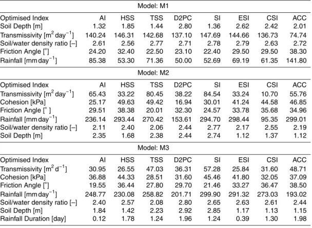
mal parameter sets are slightly different among the models and among the optimized

GOF indices for a fixed model. Moreover a compensation effect between parameter

values is evident: high values of friction angles are related to low cohesion values or high values of critical rainfall are related to high values of soil resistance

param-eters. Considering the model M1, transmissivity value (74 m2day−1) optimizing ACC

5

is much lower compared to the transmissivity values obtained optimizing the other in-dex (around 140 m2day−1). Similar behavior is observed for the optimal rainfall value which is 148 [mm day−1] optimizing ACC and around 70 [mm day−1] optimizing the other indices. Considering the model M2, the optimal transmissivity and rainfall values op-timizing CSI (10 [m2day−1] and 95 [mm day−1]), are much lower compared the values

10

obtained optimizing the other indices (around 50 [m2day−1] and 250 [mm day−1] in av-erage). For the model M3, instead, optimal parameters present the same order of mag-nitude for all optimized indices. This suggests that the variability of the optimal

param-eter values for model M1 and M2 could be due to compensate the e_ffects of important

physical processes neglected by those models.

15

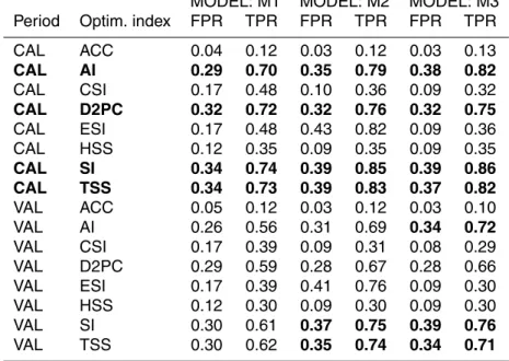
Executing the models using the eight optimal parameters set, true-positive-rates and false positive rates are computed by comparing model output and actual landslides for both calibration and verification dataset. Results were presented in Table 4, for all three models M1, M2 and M3. Those points were reported in the ROC plane in order to visualize in a unique graph the e_ffects of the optimised objective function on

20

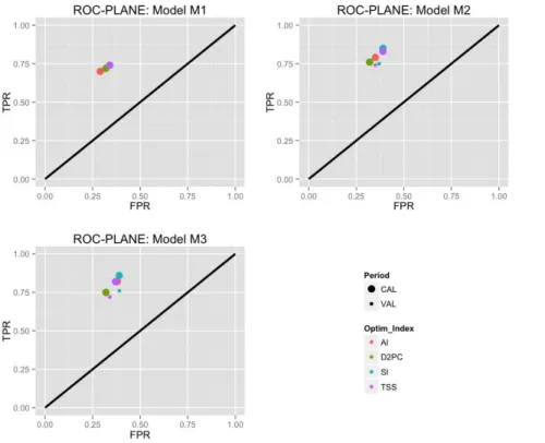
model performances. This procedure was repeated for the three models. ROC planes considering all the GOF indices and all three models are included in Figs. B1–B3 both for calibration and for verification period. For the model M2 and M3 is clear that ACC, HSS, and CSI provides the less performing models results. This is true also for model M1, even if, differently form M2 and M3, there is not a so clear separation between the

25

performances provided by ACC, HSS, and CSI and the remaining indices.

(13)

HESSD

12, 13217–13256, 2015

based models

G. Formetta et al.

Title Page

Tables Figures

◭ ◮

Back Close

Full Screen / Esc

Discussion

P

a

per

|

Discussion

P

a

per

|

Discussion

P

a

per

|

Discussion

P

a

per

|

was made in order to restrict the results’ comments only on the GOF indices that pro-vide acceptable model results and for the readability of graphs.

Figure 3 presents three ROC planes, one for each model, with the optimized GOF indices that provides FPR<0.4 and TPR>0.7. Results presented in Fig. 3 and Table 4 shows that: (i) optimization of AI, D2PC, SI and TSS allows to reach the best model

per-5

formance in the ROC plane, and this is verified for all three models, (ii) performances increase as model complexity increases: moving from M1 to M3 points in the ROC

plane approaches the perfect point (TPR=1, FPR=0), (iii) increasing model

complex-ity good model results are reached not only in calibration but also in validation dataset. In fact, moving from M1 to M2 soil cohesion and soil properties were considered, and

10

moving from M2 to M3 rainfall of finite duration was used.

The first step of the 3SVP procedure remarks that the optimization of AI, D2PC, SI, and TSS provides the best performances independently of the model we used.

3.3 Models performances correlations assessment

The second step of the procedure aims to verify the information content of each

opti-15

mized OF, checking if it is analogous to other metrics or it is peculiar of the optimized OF.

Executing a model using one of the eight parameters set (let’s assume, for example, the one obtained optimizing CSI) allows the computation of all the remaining GOF indices, that we indicate as CSICSI, ACCCSI, HSSCSI, TSSCSI, AICSI, SICSI, D2PCCSI, 20

ESI_CSI, both for calibration and for verification dataset. Let’s denote this vector with the

name MPCSI: the model performances (MP) vector computed using the parameters

set that optimize CSI. MPCSI has 16 elements, 8 for calibration and 8 for validation

dataset. Repeating the same procedure for all eight GOF indices it gives: MPACC,

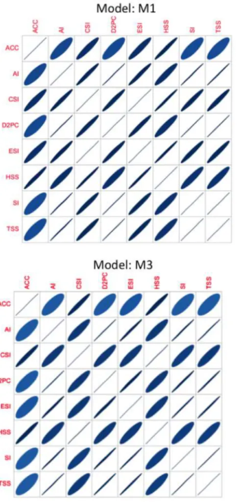
MPESI,MPSI,MPD2PC,MPTSS,MPAI,MPHS. Figure 4 presents the correlation plots 25

(Murdoch and Chow, 1996) between all MP vectors, for each model M1, M2 and M3.

The matrix is symmetric and gives a certain ellipse at intersection of rowi and column

(14)

HESSD

12, 13217–13256, 2015

based models

G. Formetta et al.

Title Page

Tables Figures

◭ ◮

Back Close

Full Screen / Esc

Discussion

P

a

per

|

Discussion

P

a

per

|

Discussion

P

a

per

|

Discussion

P

a

per

MPj vectors. The ellipse’s eccentricity is scaled according to the correlation value: the

more is prominent as the less the vector are correlated; if ellipse leans towards the right correlation is positive and if it leans to the left, it is negative.

All indices present a positive correlation among each other independent of the model

used. Moreover strong correlations between theMP vectors of AI, D2PC, SI and TSS

5

are evident in Fig. 4. This confirms that an optimization of AI, D2PC, SI and TSS provide quite similar model performances, and this is independent of the model used. On the other hand the remaining GOF indices give quite different information from the previous four indices, but they gave worse performances in first step analysis. Thus in the case study using one of the four best GOF can be enough for parameter estimation.

10

3.4 Models sensitivity assessment

In this step we focused the attention on the models M2 and M3 and we performed a parameter sensitivity analysis. Let’s assume to consider model M2 and the optimal parameter set computed by optimizing the Critical Success Index (CSI). Moreover let’s assume to consider the cohesion model parameter, the procedure evolves according

15

the following steps:

– The starting parameter values are the optimal values derived from the

optimiza-tion of the CSI index.

– All the parameters except the analyzed parameter (cohesion) were kept constant

and equal to the optimal parameter set.

20

– 1000 random values of the analyzed parameter (cohesion) were picked up from

(15)

HESSD

12, 13217–13256, 2015

based models

G. Formetta et al.

Title Page

Tables Figures

◭ ◮

Back Close

Full Screen / Esc

Discussion

P

a

per

|

Discussion

P

a

per

|

Discussion

P

a

per

|

Discussion

P

a

per

|

– 1000 values of the selected GOF index (CSI), computed by comparing model

outputs with measured data, were used to compute a boxplot of the parameterC

and optimized index CSI.

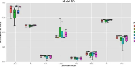
The procedure was repeated for each parameter and for each optimized index. Results where presented in Figs. 5 and 6 for model M2 and M3 respectively.

5

Each column of the figures represents one optimized index and has a number of boxplot equal to the number of model’s parameters (5 for M2 and 6 for M3). Each boxplot represents the range of variation of the optimized index due a certain model parameters change. The more narrow are the boxplot for a given optimized index the less sensitive is the model to that parameter. For both M2 and M3 the parameter set

10

obtained by optimizing AI and SI shows the less sensitive behavior for almost all pa-rameters. In this case a model parameter perturbation does not influence much the model performances. On the contrary, the models whit parameters obtained by opti-mizing ACC, TSS, and D2PC are the more sensitive to the parameters variations and this is reflected in much more evident changing of model performances.

15

3.5 Models selections and susceptibility maps

The selection of the more appropriate model for computing landslide susceptibility maps is based on what we learn forms the previous steps. In the first step we learn that (i) optimization of AI, D2PC, SI and TSS outperform the remaining indices and (ii) models M2 and M3 provides more accurate results compared to M1. The second

20

step suggests that overall models results obtained by optimizing AI, D2PC, SI and TSS are similar each others. Lastly, the third step show that models performance derived from the optimization of AI and SI are the less sensible to input variations compared to D2PC and TSS. This behavior could be due the formulation of AI and SI that gives much more weight to the true positive compared to D2PC and TSS.

25

(16)

HESSD

12, 13217–13256, 2015

based models

G. Formetta et al.

Title Page

Tables Figures

◭ ◮

Back Close

Full Screen / Esc

Discussion

P

a

per

|

Discussion

P

a

per

|

Discussion

P

a

per

|

Discussion

P

a

per

flat response changing the parameters value. A more sensitive couple model-optimal parameter set will in fact accommodates eventual parameters, input data, or measured data variations responding to these changes with a variation of model performance.

For this reason we used the combination the model M3 whit parameters obtained by optimizing D2PC for drawing the final susceptibility maps in Fig. 7. Categories of

5

landslides susceptibility from class 1 to 5 are assigned from low to high according FS values (e.g. Huang et al., 2007): Class 1 (FS<1.0), Class 2 (1.0<FS<1.2), Class 3 (1.2<FS<1.5), Class 4 (1.5<FS<2.0), Class 5 (FS>2).

4 Conclusions

The paper presents a procedure for landslides susceptibility models evaluation and

se-10

lection. It includes 3 steps: (i) model parameters calibration optimizing different GOF indices and models evaluation in the ROC plane, (ii) computation of degree of

similar-ities between different models performances obtained by optimizing all the considered

GOF index, (iii) evaluation of models sensitivity to parameters variations.

The procedure has been conceived like a model configuration of the hydrological

15

system NewAge-JGrass; it integrates: (i) three simplified physically based landslides susceptibility models, (ii) a package for model evaluations based on pixel-by-pixel com-parison of modeled and actual landslides maps, (iii) models parameters calibration al-gorithms, and (iv) the integration with uDig open-source geographic information system for model input-output maps management.

20

This procedure was applied in a test case on the Salerno-Reggio Calabria highway and the best model performances were provided by model M3 optimizing D2PC index. The system is open-source and available at (https://github.com/formeppe). It is in-tegrated according the Object Modeling System standards and this allow the user to easily integrate a generic landslide susceptibility model and use the complete

frame-25

(17)

HESSD

12, 13217–13256, 2015

based models

G. Formetta et al.

Title Page

Tables Figures

◭ ◮

Back Close

Full Screen / Esc

Discussion

P

a

per

|

Discussion

P

a

per

|

Discussion

P

a

per

|

Discussion

P

a

per

|

be improved by adding new landslide susceptibility models or different types of model

selection procedure.

Appendix A

A1 Critical Success Index (CSI)

CSI, Eq. (A1), is the number of correct detected lindslided pixels (tp), divided by the

5

sum of tp, fn and fp. CSI is also named threat score. It range between 0 and 1 and its best value is 1. It penalizes both fn and fp.

CSI= tp

tp+fp+fn (A1)

A2 Equitable Success Index (ESI)

ESI, Eq. (A2), contrarily to CSI, is able to take into account the true positives associated

10

with random chance (R). ESI ranges between−1/3 and 1. Value 1 indicates perfect

score.

ESI₌ tp−R

tp+fp+fn−R (A2)

R=(tp+fn)×(tp+fp)

tp+fn+fp+tn (A3)

A3 Success Index (SI)

15

(18)

HESSD

12, 13217–13256, 2015

based models

G. Formetta et al.

Title Page

Tables Figures

◭ ◮

Back Close

Full Screen / Esc

Discussion

P

a

per

|

Discussion

P

a

per

|

Discussion

P

a

per

|

Discussion

P

a

per

SI=1

2×

_tp

tp+fn+ tn fp+tn

=1

2×(TPR+specificity) (A4)

TPR= tp

tp₊fn (A5)

FPR= fp

fp+tn (A6)

A4 Distance to perfect classification (D2PC)

D2PC is defined in Eq. (A7). It measure the distance, in the plane FPR-TPR between

5

an ideal perfect point of coordinates (0,1) and the point of the tested model (FPR,TPR). D2PC ranges in 0–1 and its best value are 0.

D2PC=

q

(1−TPR)2+FPR2 (A7)

A5 Average Index (AI)

AI, Eq. (A8), is the average value between four different indices: (i) TPR, (ii) precision,

10

(iii) the ratio between successfully predicted stable pixels (tn) and the total number of

actual stable pixels (fp+tn) and (iv) the ratio between successfully predicted stable

pixels (tn) and the number of simulated stable cells (fn+tn).

AI=1

4

_tp

tp+fn+ tp tp+fp+

tn fp+tn+

tn fn+tn

(A8)

A6 Heidke Skill Score (HSS)

15

(19)

HESSD

12, 13217–13256, 2015

based models

G. Formetta et al.

Title Page

Tables Figures

◭ ◮

Back Close

Full Screen / Esc

Discussion

P

a

per

|

Discussion

P

a

per

|

Discussion

P

a

per

|

Discussion

P

a

per

|

Ma, the skill score formulation is expressed in Eq. (A9):

SS= Ma−Mc

Mopt−Mc

(A9)

where Mc is the control or reference model accuracy and Mopt is the perfect model

accuracy.

SS assumes positive and negative value, if the tested model is perfectMa=Moptand 5

SS=1, if the tested model is equal to the control model thanMa=Mcand SS=0.

The marginal probability of a predicted unstable pixel is (tp+fp)/nwherenis the total number of pixelsn=tp+fn+fp+tn. The marginal probability of a landslided unstable pixel is (tp+fn)/n.

The probability of a correct yes forecast by chance is: P1=(tp+fp)(tp+fn)/n2. The

10

probability of a correct no forecast by chance is: P2=(tn+fp)(tn+fn)/n2.

In the HSS, Eq. (A10), the control model is a model that forecast by chance:Mc=

P1+P2, the measure of accuracy is the Accuracy (ACC) defined in Eq. (A11), and the

Mopt=1.

HSS= 2×(tp×tn)−(fp×fn)

(tp+fn)×(fn+tn)₊(tp+fp)×(fp+tn) (A10)

15

ACC= tp+tn

tp+fn+fp+tn (A11)

The range of the HSS is−∞to 1. Negative values indicate that indicates that the model

provides no better results of a random model, 0 means no model skill, and a perfect model obtains a HSS of 1. HSS is also named as Cohen’s kappa.

A7 True Skill Statistic (TSS)

20

(20)

HESSD

12, 13217–13256, 2015

based models

G. Formetta et al.

Title Page

Tables Figures

◭ ◮

Back Close

Full Screen / Esc

Discussion

P

a

per

|

Discussion

P

a

per

|

Discussion

P

a

per

|

Discussion

P

a

per

−1 and 1 and its best value is 1. TSS equal −1 indicates that the model provides no

better results of a random model. A TSS equal 0 indicates an indiscriminate model. TSS measures the ability of the model to distinguish between landslided and non-landslided pixels. If the number of tn is large the false alarm value is relatively over-whelmed. If tn is large, as happens in landslides maps, FPR tends to zero and TSS

5

tends to TPR. A problem of TSS is that it threats the hit rate and the false alarm rate equally, irrespective of their likely differing consequences.

TSS=(tp×tn)−(fp×fn)

(tp+fn)×(fp+tn) =TPR−FPR (A12)

TSS is similar to Heidke, except the constraint on the reference forecasts is that they are constrained to be unbiased.

10

Acknowledgements. This research was funded by PON Project No. 01_01503 “Integrated Sys-tems for Hydrogeological Risk Monitoring, Early Warning and Mitigation Along the Main Life-lines”, CUP B31H11000370005, in the framework of the National Operational Program for “Re-search and Competitiveness” 2007–2013.

References 15

Abera, W., Antonello, A., Franceschi, S., Formetta, G., and Rigon, R.: “The uDig Spatial Toolbox for hydro-geomorphic analysis”, in: Geomorphological Techniques, v. 4, n. 1, 1– 19, available at: http://www.geomorphology.org.uk/sites/default/files/geom_tech_chapters/2. 4.1_GISToolbox.pdf (last access: December 2015), 2014.

Baum, R., Savage, W., and Godt, J.: TRIGRS, a Fortran Program for Transient Rainfall

Infil-20

tration and Grid-Based Regional Slope-Stability Analysis, US Geological Survey Open Re-port 424, US Geological Survey, Golden, CO, 61 pp., 2002.

Beguería, S.: Validation and evaluation of predictive models in hazard assessment and risk management, Nat. Hazards, 37, 315–329, 2006.

Bennett, N. D., Croke, B. F., Guariso, G., Guillaume, J. H., Hamilton, S. H., Jakeman, A. J.,

25

(21)

HESSD

12, 13217–13256, 2015

based models

G. Formetta et al.

Title Page

Tables Figures

◭ ◮

Back Close

Full Screen / Esc

Discussion

P

a

per

|

Discussion

P

a

per

|

Discussion

P

a

per

|

Discussion

P

a

per

|

Borga, M., Dalla Fontana, G., and Cazorzi, F.: Analysis of topographic and climatic control on rainfall-triggered shallow landsliding using a quasi-dynamic wetness index, J. Hydrol., 268, 56–71, 2002.

Brabb, E. E.: Innovative approaches to landslide hazard and risk mapping, in: Proceedings of the 4th International Symposium on Landslides, 16–21 September, Toronto, Ontario,

5

Canada, Canadian Geotechnical Society, Toronto, Ontario, Canada, 1, 307–324, 1984. Brown, C. D. and Davis, H. T.: Receiver operating characteristics curves and related decision

measures: a tutorial, Chemometr. Intell. Lab., 80, 24–38, 2006.

Capparelli, G. and Versace, P.: FLaIR and SUSHI: two mathematical models for early warning of landslides induced by rainfall, Landslides, 8, 67–79, 2011.

10

Capparelli, G., Iaquinta, P., Iovine, G. G. R., Terranova, O. G., and Versace, P.: Modelling the rainfall-induced mobilization of a large slope movement in northern Calabria, Nat. Hazards, 61, 247–256, 2012.

Cascini, L., Bonnard, C., Corominas, J., Jibson, R., and Montero-Olarte, J.: Landslide hazard and risk zoning for urban planning and development, in: Landslide Risk Management, Taylor

15

and Francis, London, 199–235, 2005.

Catani, F., Casagli, N., Ermini, L., Righini, G., and Menduni, G.: Landslide hazard and risk mapping at catchment scale in the Arno River basin, Landslides, 2, 329–342, 2005.

Chung, C.-J. F., Fabbri, A. G. and van Westen, C. J.: Multivariate regression analysis for land-slide hazard zonation, in: Geographical Information Systems in Assessing Natural Hazards,

20

edited by: Carrara, A. and Guzzetti, F., Kluwer Academic Publishers, Dordrecht, 107–34, 1995.

Colella, A., De Boer, P. L., and Nio, S. D.: Sedimentology of a marine intermontane Pleistocene Gilbert-type fan-delta complex in the Crati Basin, Calabria, southern Italy, Sedimentology, 34, 721–736, 1987.

25

Conforti, M., Aucelli, P. P. C., Robustelli, G., and Scarciglia, F.: Geomorphology and GIS analysis for mapping gully erosion susceptibility in the Turbolo Stream catchment (Northern Calabria, Italy), Nat. Hazards, 56, 881–898, 2011.

Conforti, M., Pascale, S., Robustelli, G., and Sdao, F.: Evaluation of prediction capability of the artificial neural networks for mapping landslide susceptibility in the Turbolo River catchment

30

(22)

HESSD

12, 13217–13256, 2015

based models

G. Formetta et al.

Title Page

Tables Figures

◭ ◮

Back Close

Full Screen / Esc

Discussion

P

a

per

|

Discussion

P

a

per

|

Discussion

P

a

per

|

Discussion

P

a

per

Corominas, J., Van Westen, C., Frattini, P., Cascini, L., Malet, J. P., Fotopoulou, S., Catani, F., Van Den Eeckhaut, M., Mavrouli, O., Agliardi, F., and Pitilakis, K.: Recommendations for the quantitative analysis of landslide risk, B. Eng. Geol. Environ., 73, 209–263, 2014.

David, O., Ascough II, J. C., Lloyd, W., Green, T. R., Rojas, K. W., Leavesley, G. H., and Ahuja, L. R.: A software engineering perspective on environmental modeling framework

de-5

sign: the Object Modeling System, Environ. Modell. Softw., 39, 201–213, 2013.

Dietrich, W. E., Bellugi, D., and Real De Asua, R.: Validation of the Shallow Landslide Model, SHALSTAB, for forest management, in: Land Use and Watersheds: Human Influence on Hydrology and Geomorphology in Urban and Forest Areas, edited by: Wigmosta, M. S. and Burges, S. J., American Geophysical Union, Washington, D.C., doi:10.1029/WS002p0195,

10

2001.

Duan, Q., Sorooshian, S., and Gupta, V.: Effective and efficient global optimization for concep-tual rainfall–runo_ffmodels, Water Resour. Res., 28, 1015–1031, 1992.

Duncan, J. M. and Wright, S. G.: Soil Strength and Slope Stability, John Wiley, New Jersey, 297 pp., 2005.

15

Fabbricatore, D., Robustelli, G., and Muto, F.: Facies analysis and depositional architecture of shelf-type deltas in the Crati Basin (Calabrian Arc, south Italy), Boll. Soc. Geol. Ital., 133, 131–148, 2014.

Formetta, G., Mantilla, R., Franceschi, S., Antonello, A., and Rigon, R.: The JGrass-NewAge system for forecasting and managing the hydrological budgets at the basin scale: models of

20

flow generation and propagation/routing, Geosci. Model Dev., 4, 943–955, doi:10.5194/gmd-4-943-2011, 2011.

Formetta, G., Antonello, A., Franceschi, S., David, O., and Rigon, R.: Hydrological modelling with components: a GIS-based open-source framework, Environ. Modell. Softw., 55, 190– 200, 2014.

25

Formetta, G., Capparelli, G., Rigon, R., and Versace, P.: Physically based landslide suscepti-bility models with different degree of complexity: calibration and verification, in: International Environmental Modelling and Software Society (iEMSs), 7th Intl. Congress on Env. Mod-elling and Software, San Diego, CA, USA, edited by: Ames, D. P., Quinn, N. W. T., and Rizzoli, A. E., available at: http://www.iemss.org/society/index.php/iemss-2014-proceedings,

30

last access: December 2015.

(23)

HESSD

12, 13217–13256, 2015

based models

G. Formetta et al.

Title Page

Tables Figures

◭ ◮

Back Close

Full Screen / Esc

Discussion

P

a

per

|

Discussion

P

a

per

|

Discussion

P

a

per

|

Discussion

P

a

per

|

Glade, T. and Crozier, M. J.: A review of scale dependency in landslide hazard and risk analysis, Landslide Hazard Risk, 3, 75–138, 2005.

Goodenough, D. J., Rossmann, K., and Lusted, L. B.: Radiographic applications of receiver operating characteristic (ROC) analysis, Radiology, 110, 89–95, 1974.

Grahm, J.: Methods of slope stability analysis, in: Slope Instability, edited by: Brunsden, D. and

5

Prior, D. B., Wiley, New York, 171–215, 1984.

Guzzetti, F., Reichenbach, P., Ardizzone, F., Cardinali, M., and Galli, M.: Estimating the quality of landslide susceptibility models, Geomorphology, 81, 166–184, 2006.

Hay, L. E., Leavesley, G. H., Clark, M. P., Markstrom, S. L., Viger, R. J., and Umemoto, M.: Step-wise, multiple-objective calibration of a hydrologic model for a snowmelt-dominated basin, J.

10

Am. Water Resour. As., 42, 877–890, 2006.

Huang, J.-C., Kao, S.-J., Hsu, M.-L., and Liu, Y.-A.: Influence of Specific Contributing Area algorithms on slope failure prediction in landslide modeling, Nat. Hazards Earth Syst. Sci., 7, 781–792, doi:10.5194/nhess-7-781-2007, 2007.

Hutchinson, J. N.: Keynote paper: landslide hazard assessment, in: Landslides, edited by: Bell,

15

D. H., Balkema, Rotterdam, 1805–1841, 1995.

Iovine, G. G. R., Lollino, P., Gariano, S. L., and Terranova, O. G.: Coupling limit equilibrium anal-yses and real-time monitoring to refine a landslide surveillance system in Calabria (south-ern Italy), Nat. Hazards Earth Syst. Sci., 10, 2341–2354, doi:10.5194/nhess-10-2341-2010, 2010.

20

Iverson R. M.: Landslide triggering by rain infiltration, Water Resour. Res., 36, 1897–1910, 2000.

Jolliffe, I. T. and Stephenson, D. B. (Eds.): Forecast Verification: a Practitioner’s Guide in Atmo-spheric Science, John Wiley and Sons, Exeter, UK, 2012.

Kennedy, J. and Eberhart, R.: Particle swarm optimization, in: Proceedings of IEEE

Interna-25

tional Conference on Neural Networks, Vol. 4, Perth, WA, 1995.

Lanzafame, G. and Tortorici, L.: La tettonica recente del Fiume Crati (Calabria), Geogr. Fis. Din. Quat., 4, 11–21, 1984.

Lee, S., Chwae, U., and Min, K.: Landslide susceptibility mapping by correlation between to-pography and geological structure: the Janghung area, Korea, Geomorphology, 46, 149–162,

30

2002.

(24)

HESSD

12, 13217–13256, 2015

based models

G. Formetta et al.

Title Page

Tables Figures

◭ ◮

Back Close

Full Screen / Esc

Discussion

P

a

per

|

Discussion

P

a

per

|

Discussion

P

a

per

|

Discussion

P

a

per

Montgomery, D. R. and Dietrich, W. E.: A physically based model for the topographic control on shallow landsliding, Water Resour. Res., 30, 1153–1171, 1994.

Murdoch, D. J. and Chow, E. D.: A graphical display of large correlation matrices, Am. Stat., 50, 178–180, 1996.

Naranjo, J. L., van Westen, C. J., and Soeters, R.: Evaluating the use of training areas in

5

bivariate statistical landslide hazard analysis: a case study in Colombia, ITC J., 3, 292–300, 1994.

Park, H. J., Lee, J. H., and Woo, I.: Assessment of rainfall-induced shallow landslide suscepti-bility using a GIS-based probabilistic approach, Eng. Geol., 161, 1–15, 2013.

Park, N. W.: Application of Dempster–Shafer theory of evidence to GIS-based landslide

sus-10

ceptibility analysis, Environ. Earth Sci., 62, 367–376, 2011.

Pepe, M. S.: The Statistical Evaluation of Medical Tests for Classification and Prediction, Oxford University Press, New York, 2003.

Petschko, H., Brenning, A., Bell, R., Goetz, J., and Glade, T.: Assessing the quality of landslide susceptibility maps – case study Lower Austria, Nat. Hazards Earth Syst. Sci., 14, 95–118,

15

doi:10.5194/nhess-14-95-2014, 2014.

Provost, F. and Fawcett, T.: Robust classification for imprecise environments, Mach. Learn., 42, 203–231, 2001.

Rosso, R., Rulli, M. C., and Vannucchi, G.: A physically based model for the hydrologic con-trol on shallow landsliding, Water Resour. Res., 42, W06410, doi:10.1029/2005WR004369,

20

2006.

Sidle, R. C. and Ochiai, H.: Landslides: Processes, Prediction, and Land Use, Vol. 18, American Geophysical Union, Washington, D.C., 2006.

Simoni, S., Zanotti, F., Bertoldi, G., and Rigon, R.:: Modeling the probability of occurrence of shallow landslides and channelized debris flows using GEOtop-FS, Hydrol. Process., 22,

25

532–545, 2008.

Varnes, D. J. and IAEG Commission on Landslides and other Mass Movements, Landslide Hazard Zonation: a Review of Principles and Practice, UNESCO Press, Paris, 63 pp., 1984. Vezzani, L.: I terreni plio-pleistocenici del basso Crati (Cosenza), Atti dell’Accademia Gioenia

di Scienze Naturali di Catania, 6, 28–84, 1968.

30

(25)

HESSD

12, 13217–13256, 2015

based models

G. Formetta et al.

Title Page

Tables Figures

◭ ◮

Back Close

Full Screen / Esc

Discussion

P

a

per

|

Discussion

P

a

per

|

Discussion

P

a

per

|

Discussion

P

a

per

|

Wu, W. and Sidle, R. C.: A distributed slope stability model for steep forested basins, Water Resour. Res., 31, 2097–2110, doi:10.1029/95WR01136, 1995.

Young, J. and Colella, A.: Calcarenous nannofossils from the Crati Basin, in: Fan Deltas-Excursion Guidebook, edited by: Colella, A., Università della Calabria, Cosenza, Italy, 79–96, 1988.

(26)

HESSD

12, 13217–13256, 2015

based models

G. Formetta et al.

Title Page

Tables Figures

◭ ◮

Back Close

Full Screen / Esc

Discussion

P

a

per

|

Discussion

P

a

per

|

Discussion

P

a

per

|

Discussion

P

a

per

Table 1.Indices of goodness of fit for comparison between actual and predicted landslide.

Name Definition Range Optimal value

Critical success index (CSI) CSI= _tp+fp+fntp [0,1] 1.0

Equitable success index (ESI) ESI=_tp+fp+fntp−R−R R=

(tp+fn)×(tp+fp)

tp+fn+fp+tn [−1/3, 1] 1.0

Success Index (SI) SI=1₂×

_tp tp+fn+

tn fp+tn

[0,1] 1.0

Distance to perfect D2PC=

q

(1−TPR)2+FPR2 [0,1] 0.0

classification (D2PC) TPR=tptp+fn FPR=

fp fp+tn

Average Index (AI) AI=1

4 _tp

tp+fn+ tp tp+fp+

tn fp+tn+

tn fn+tn

[0,1] 1.0

True skill statistic (TSS) TSS=(tp×tn)−(fp×fn)

(tp+fn)×(fp+tn) [−1, 1] 1.0

Heidke skill score (HSS) HSS= 2×(tp×tn)−(fp×fn)

(tp+fn)×(fn+tn)+(tp+fp)×(fp+tn) [−∞, 1] 1.0

(27)

HESSD

12, 13217–13256, 2015

based models

G. Formetta et al.

Title Page

Tables Figures

◭ ◮

Back Close

Full Screen / Esc

Discussion

P

a

per

|

Discussion

P

a

per

|

Discussion

P

a

per

|

Discussion

P

a

per

|

Table 2.Optimised models’ parameters values.

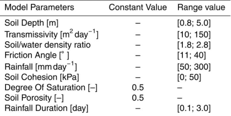
Model Parameters Constant Value Range value

(28)

HESSD

12, 13217–13256, 2015

based models

G. Formetta et al.

Title Page

Tables Figures

◭ ◮

Back Close

Full Screen / Esc

Discussion

P

a

per

|

Discussion

P

a

per

|

Discussion

P

a

per

|

Discussion

P

a

per

Table 3.Optimal parameter sets output of the optimization procedure of each GOF indices in turn. Results were presented for each model (M1, M2 and M3).

Model: M1

Optimised Index AI HSS TSS D2PC SI ESI CSI ACC

Soil Depth [m] 1.32 1.85 1.44 2.80 1.36 2.62 2.42 2.01

Transmissivity [m2day−1

] 140.24 146.31 142.68 137.10 147.69 144.66 136.73 74.74

Soil/water density ratio [–] 2.61 2.56 2.77 2.71 2.78 2.79 2.63 2.72

Friction Angle [◦

] 24.20 32.40 22.50 23.10 22.40 29.50 29.50 38.30

Rainfall [mm day−1_] _85.38 _53.30 _71.36 _50.00 _52.69 _69.19 _61.35 _141.80

Model: M2

Transmissivity [m2day−1] 65.43 33.22 80.45 38.22 84.54 33.24 10.70 55.76

Cohesion [kPa] 25.17 49.63 49.42 16.94 30.01 41.24 44.58 46.85

Friction Angle [◦

] 29.51 38.38 20.01 32.30 24.57 33.78 35.68 34.96

Rainfall [mm day−1

] 236.14 293.44 270.42 153.61 294.70 298.44 95.35 299.01

Soil Depth [m] 2.35 1.68 2.38 2.44 2.74 1.12 1.37 1.12

Model: M3

Transmissivity [m2d−1

] 30.95 26.55 47.03 36.31 57.28 25.84 31.60 48.71

Cohesion [kPa] 36.88 44.33 28.51 31.60 45.46 41.80 32.05 37.09

Friction Angle [◦

] 19.55 36.44 27.80 29.70 21.46 33.27 36.47 38.50

Rainfall [mm day−1_] _248.77 _230.08 _258.82 _201.71 _299.90 _291.32 _273.03 _193.02

Soil Depth [m] 1.84 1.42 2.23 2.92 2.85 1.17 1.13 1.15

(29)

HESSD

12, 13217–13256, 2015

based models

G. Formetta et al.

Title Page

Tables Figures

◭ ◮

Back Close

Full Screen / Esc

Discussion

P

a

per

|

Discussion

P

a

per

|

Discussion

P

a

per

|

Discussion

P

a

per

|

Table 4.Results in term of true-positive rate (TPR) and false-positive rate (FPR), for each model (M1, M2 and M3), for each optimised GOF index and for both calibration and verification dataset. In bold the rows for which the condition FPR<0.4 and TPR>0.7 is verified.

MODEL: M1 MODEL: M2 MODEL: M3 Period Optim. index FPR TPR FPR TPR FPR TPR

CAL ACC 0.04 0.12 0.03 0.12 0.03 0.13

CAL AI 0.29 0.70 0.35 0.79 0.38 0.82

CAL CSI 0.17 0.48 0.10 0.36 0.09 0.32

CAL D2PC 0.32 0.72 0.32 0.76 0.32 0.75

CAL ESI 0.17 0.48 0.43 0.82 0.09 0.36 CAL HSS 0.12 0.35 0.09 0.35 0.09 0.35

CAL SI 0.34 0.74 0.39 0.85 0.39 0.86 CAL TSS 0.34 0.73 0.39 0.83 0.37 0.82

VAL ACC 0.05 0.12 0.03 0.12 0.03 0.10 VAL AI 0.26 0.56 0.31 0.69 0.34 0.72

VAL CSI 0.17 0.39 0.09 0.31 0.08 0.29 VAL D2PC 0.29 0.59 0.28 0.67 0.28 0.66 VAL ESI 0.17 0.39 0.41 0.76 0.09 0.30 VAL HSS 0.12 0.30 0.09 0.30 0.09 0.30 VAL SI 0.30 0.61 0.37 0.75 0.39 0.76

(30)

HESSD

12, 13217–13256, 2015

based models

G. Formetta et al.

Title Page

Tables Figures

◭ ◮

Back Close

Full Screen / Esc

Discussion

P

a

per

|

Discussion

P

a

per

|

Discussion

P

a

per

|

Discussion

P

a

per

Table A1.Acronyms table.

3SVP Three steps verification procedure

AI Average Index

CSI Critical success index

D2PC Distance to perfect classification

ESI Equitable success index

fn False negative

fp False positive

FPR False positive rate

FS Factor of safety

GIS Geogrphic informatic system

GOF Goodness of fit indices

HSS Heidke skill score

LSA Landslide susceptibility analysis

M1 Model for landslide susceptibility analysis proposed

in Montgomery and Dietrich (1994)

in Park et al. (2013)

in Rosso et al. (2006)

MP Model performances vector

OF Objective function

OL Observed landslide map

OMS Object modeling system

PL Predicted landslide map

PSO Particle Swarm optimization

ROC Receiver operating characteristic

SI Success index

TCA Total contributing area

tn True negative

tp True positive

TPR True positive rate

(31)

HESSD

12, 13217–13256, 2015

based models

G. Formetta et al.

Title Page

Tables Figures

◭ ◮

Back Close

Full Screen / Esc

Discussion

P

a

per

|

Discussion

P

a

per

|

Discussion

P

a

per

|

Discussion

P

a

per

|

(32)

HESSD

12, 13217–13256, 2015

based models

G. Formetta et al.

Title Page

Tables Figures

◭ ◮

Back Close

Full Screen / Esc

Discussion

P

a

per

|

Discussion

P

a

per

|

Discussion

P

a

per

|

Discussion

P

a

per

(33)

HESSD

12, 13217–13256, 2015

based models

G. Formetta et al.

Title Page

Tables Figures

◭ ◮

Back Close

Full Screen / Esc

Discussion

P

a

per

|

Discussion

P

a

per

|

Discussion

P

a

per

|

Discussion

P

a

per

|

(34)

HESSD

12, 13217–13256, 2015

based models

G. Formetta et al.

Title Page

Tables Figures

◭ ◮

Back Close

Full Screen / Esc

Discussion

P

a

per

|

Discussion

P

a

per

|

Discussion

P

a

per

|

Discussion

P

a

per