www.atmos-meas-tech.net/9/1369/2016/ doi:10.5194/amt-9-1369-2016
© Author(s) 2016. CC Attribution 3.0 License.
Profiling the PM
2
.
5
mass concentration vertical
distribution in the boundary layer
Zongming Tao1,2, Zhenzhu Wang2, Shijun Yang1, Huihui Shan1, Xiaomin Ma1, Hui Zhang1, Sugui Zhao1, Dong Liu2, Chenbo Xie2, and Yingjian Wang2,3
1New Star Institute of Applied Technology, Hefei, Anhui 230031, China
2Key Laboratory of Atmospheric Composition and Optical Radiation, Anhui Institute of Optics and Fine Mechanics, Chinese Academy of Sciences, Hefei, Anhui 230031, China
3University of Science and Technology of China, Hefei, Anhui 230031, China
Correspondence to:Zhenzhu Wang ([email protected])
Received: 16 September 2015 – Published in Atmos. Meas. Tech. Discuss.: 9 December 2015 Revised: 2 March 2016 – Accepted: 16 March 2016 – Published: 1 April 2016
Abstract. Fine particles (PM2.5) affect human life and ac-tivities directly; the detection of PM2.5 mass concentration profile is very essential due to its practical and scientific sig-nificance (such as the quantification of air quality and its variability as well as the assessment of improving air quality forecast). But so far, it has been difficult to detect PM2.5mass concentration profile. The proposed methodology to study the relationship between aerosol extinction coefficient and PM2.5mass concentration is described, which indicates that the PM2.5 mass concentration profile could be retrieved by combining a charge-coupled device (CCD) side-scatter lidar with a PM2.5sampling detector. When the relative humidity is less than 70 %, PM2.5, mass concentration is proportional to the aerosol extinction coefficient, and then the specific co-efficient can be calculated. Through this specific coco-efficient, aerosol extinction profile is converted to PM2.5mass concen-tration profile. Three cases of clean night (on 21 September 2014), pollutant night (on 17 March 2014), and heavy pollu-tant night (on 13 February 2015) are studied. The character-istics of PM2.5mass concentration profile at the near-ground level during the cases of these 3 nights in the western suburb of Hefei city were discussed. The PM2.5air pollutant concen-tration is comparatively large close to the surface and varies with time and altitude. The experiment results show that the CCD side-scatter lidar combined with a PM2.5detector is an effective and new method to explore pollutant mass concen-tration profile at the near-ground level.
1 Introduction
Atmospheric aerosol is defined as suspended particle in the air, and its size distributes from 0.001 to 100 µm in diame-ter in liquid or solid state. Fine particles (PM2.5) constitute a particular group of particle, whose size is less than 2.5 µm in diameter; it is an important part of aerosol. PM2.5are also called fine particles because of their small size. PM2.5is con-sidered to be the most serious pollutant in the urban areas all over the world due to its adverse health effects, including cardiovascular diseases, respiratory irritation, and pulmonary dysfunction (An et al., 2000; Mao et al., 2002; Xu et al., 2007). The PM2.5poses great health risks, compared to the coarse particle matter, because the increased surface areas have a high potential to adsorb or condense toxic air pollu-tants (An et al., 2000). Meanwhile PM2.5can degrade the at-mospheric visibility and affect traffic safety by the extinction effect. In recent years, a series of experiments or monitors about fine particle matter are researched in many mega cities in China by institutes (Mao et al., 2002; Che et al., 2015), and the results indicated that the PM2.5mass concentration was increased.
information for model evaluation, improvement, and devel-opment for the daily air quality forecast.
Currently, the direct detecting device for PM2.5is the parti-cle matter sampling monitor, which is mostly installed on the surface ground. Using the meteorological tower, only a few researchers fitted PM2.5monitors at different altitudes in Bei-jing and Tianjin to get the profile of PM2.5mass concentra-tion within 325 m (Wu et al., 2009; Yang et al., 2005). So it is difficult to obtain PM2.5mass concentration profile in a few kilometers. However, some important atmospheric processes (i.e. particle formation, transportation and mixing processes) take place predominantly at a higher altitude in the plane-tary boundary layer. Lidar, in principle, can provide the abil-ity to observe these processes where they occur. Backscat-tering lidar is a powerful tool to detect aerosol profile, and is widely used in atmospheric monitoring (Weitkamp, 2005; Winker et al., 2007; Bo et al., 2014; Wang et al., 2014b). But the common backscattering lidar system has a shortcoming in the lower hundreds of meters because of the geometric form factor (GFF) caused by the configuration of the trans-mitter divergence and receiver’s field of view (FOV) at the near range (Mao et al., 2012; Wang et al., 2015b). With the recently developed technique of the CCD side-scattering li-dar (Bernes et al., 2003; Tao et al., 2014a; Ma et al., 2014), the problem caused by the GFF could be solved. Moreover, the nearer range and the better spatial resolution could be obtained. So the siscattering lidar is very suitable for de-tecting aerosol spatial distribution in the boundary layer from the surface.
In this paper, the aerosol extinction coefficient profile is retrieved by our self-developed CCD side-scattering lidar, and PM2.5 mass concentration is measured simultaneously on the ground level by a particle matter monitor. Syncretiz-ing these two data sets measured at the same time and in the same place, the profile of PM2.5 mass concentration can be derived in the boundary layer. In Sect. 2, the instrumentation is introduced, and the methodology for extinction and PM2.5 profiles is shown in Sect. 3. Then the results are discussed in Sect. 4, followed by the summary and conclusion in the last Sect. 5.
2 Instruments
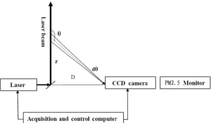
The measurement system consists of a CCD side-scattering lidar and a PM2.5mass monitor as shown in Fig. 1. The sub-system of side-scattering lidar consists of laser, CCD cam-era, geometric calibration, data acquisition and control com-puter. The light source is a Nd:YAG laser (Quantel Bril-liant) emitting laser pulses in 20 Hz at 532 nm wavelength. The side-scattering light is received by a CCD camera with 3352×2532 pixels. The exposed time is set as 5 min
accord-ing to the signal-to-noise ratio with a maximum relative er-ror of 1.5 % caused by noises (Ma et al., 2014), and there is an interference filter with 30 nm bandwidth in front of CCD lens. Through geometric calibration, the relationship
Figure 1.The diagram of the measurement system.
Table 1.The specifications of the C-lidar system.
Laser (Quantel Brilliant) Nd:YAG
Wavelength (nm) 532 Pulse energy (mJ) 200 Repetition rate (Hz) 20
Detector (SBIG) ST-8300M
Pixel array 3352×2532
Pixel size (µm) 5.4×5.4 A/D convecter (bits) 16
Wide-angle lens Walimexpro f/2.8 Lens focal length (mm) 14
CCD sensor Kodak KAF-8300
Quantum efficiency (532 nm) ∼55 %
Interference filter (Semrock corporation)
Bandwidth (nm) 25.6
Peak transmittance ∼95 %
between the pixels and the corresponding scattering lights in laser beam is determined. The computer acquires the CCD camera data and controls timing sequence between laser and CCD camera. PM2.5mass monitor works simultaneously and the output is the average PM2.5mass concentration through-out 1 hour. In Fig. 1;z is the detecting distance; D is the distance from CCD camera to laser beam;θis the scattering angle; dθis the FOV of one pixel. The detailed specifications of the CCD side-scattering lidar (C-lidar) are described in the previous work (Tao et al., 2014a) and shown in Table 1.
The PM2.5mass monitor, named Thermo Scientific TEOM 1405 Ambient Particulate Monitor, can carry out continu-ous measurement of ambient particulate concentrations with the resolution of 0.1 µg m3and the precision of±2.0 µg m3
3 Methodology
3.1 Retrieved method of aerosol extinction profile
The side-scattering lidar equation is expressed as (Tao et al., 2014b):
P (z, θ )=P0KA
D
β1(z, π )
f1(π )
f1(θ )+
β2(z, π )
f2(π )
f2(θ )
(1)
×exp −τ−τ/cos(π−θ ) dθ,
where P (z, θ ) is the received power at height z and scat-tering angle θ by a pixel, P0 is laser pulse energy, K is a system constant including the optical and electronic ef-ficiency, A is the area of CCD camera lens, D is the dis-tance from CCD camera to laser beam,β(z, π )is backscat-tering coefficient, andf (θ )is phase function. Subscripts “1” and “2” represent aerosol and molecule scattering, respec-tively. τ is optical depth,α(z)is extinction coefficient, and
τ =Rz
0(α1(z ′)+α
2(z′))dz′.
In general, for Eq. (1), there are six unknown variables, i.e. phase function, backscattering and extinction coefficients of aerosol and molecule. Three unknown variables for molecule are calculated through the standard molecular model by Rayleigh scatter theory. A prior assumption has to be given, i.e. lidar ratio (extinction-to-backscattering ratio) of aerosol, because of the principle of lidar equation. The value of 50 Sr is used as lidar ratio at 532 nm wavelength in our algo-rithm. The aerosol phase function is determined from a sky-radiometer (for example, a Prede POM-02 sky-sky-radiometer made in Japan). Then only one variable (the backscattering or extinction coefficient of aerosol) is left, which can be de-rived from Eq. (1) as follows.
In our experiment, vertical-pointing backscattering lidar (V-lidar) and C-lidar worked simultaneously. For V-lidar data processing, it is a traditional way to select the clear point about the tropopause as the reference point assumed to have minimum aerosol. The V-lidar signals and C-lidar signals have an overlap region around 1 km in height in our case. For C-lidar, the reference point is selected in this overlap re-gion. Aerosol backscatter coefficient value βc at the refer-ence point thus can be given from V-lidar retrieval. When the aerosol backscatter coefficient value at the scattering angle
θcas the reference point is known, according to Eq. (1), the backscattering or extinction coefficient of aerosol can be de-rived in our proposed numerical inversion method (Tao et al., 2014b). The validation experiments and error analysis are shown in the reference (Tao et al., 2015). When compar-ative experiments were performed, the C-lidar and V-lidar worked at the same position simultaneously, as well as an-other horizontal-pointing backscattering lidar (H-lidar). The result shown in the Fig. 2 of the reference (Tao et al., 2015) indicates a good agreement and the total relative error of ex-tinction coefficient is less than 18 % accordingly in the error propagation method and by the typical example.
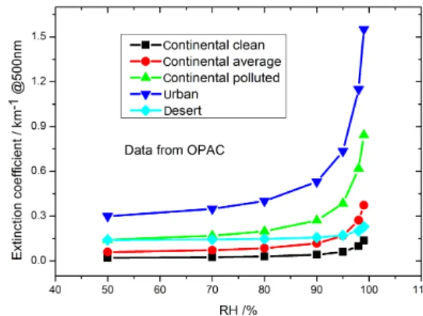
Figure 2.The relationship between aerosol extinction coefficient and atmospheric relative humidity (RH) for five types of aerosol.
3.2 Retrieved method of PM2.5profile
Some researchers (Pesch and Oderbolz, 2007; Sano et al., 2008; He et al., 2010; Cordero et al., 2012) studied the rela-tionship between the PM2.5mass concentration and aerosol optical depth by a review of statistics. The aerosol optical depth is the integral result of aerosol extinction to range, which may match the column PM2.5 mass concentration. However, the aerosol extinction and PM2.5mass concentra-tion both change along altitude. So the PM2.5mass concen-tration is closely related to the aerosol extinction in theory.
The aerosol size distributionn(r)is defined as
n(r)=dN
dr , (2)
where dN is the particle number concentration in radius in-terval range (r→r+dr).
Total particle matter mass concentrationCTotalcan be writ-ten as
CTotal= ∞ Z
0
ρ 4
3π r 3
n(r)dr, (3)
whereρis the aerosol mass density.
PM2.5mass concentrationCPM2.5can be written as
CPM2.5 = 2.5 µm
Z
0
ρ 4
3π r 3
n(r)dr. (4)
Aerosol extinction coefficientαcan be described as
α=
∞ Z
0
π r2Qextn(r)dr, (5)
whereQextis the factor of extinction efficiency.
are effective radius, i.e. the surface-area-weighted mean ra-dius as
reff= ∞ Z
0
r3n(r)dr/
∞ Z
0
r2n(r)dr. (6)
So, the relationship between aerosol extinction and total par-ticle mass concentration is determined (Li et al., 2013)
α=3Qext
4reffρ
CTotal. (7)
Using the ratio of total particle matter mass concentration to PM2.5mass concentration (η=CTotal/CPM2.5), finally we
got the following relationship:
α=3Qextη
4reffρ
CPM2.5=K×CPM2.5. (8)
Eq. (8) is the formula to convert aerosol extinction profile to PM2.5 mass concentration profile, whereK=34Qreffextρη is the specific coefficient.
In Eq. (8), the specific coefficient Kis related to aerosol size distribution, refractive index, and atmospheric relative humidity. In the planetary boundary layer (PBL), due to tur-bulence effect, the aerosol size distribution and refractive in-dex are assumed as to be reasonably uniform. When the rela-tive humidity is below 70 %, the aerosol hydrophilic growth could be negligible. So, the specific coefficient K could be considered as constant under the condition of less than 70 % relative humidity in the PBL; i.e. K is independent of alti-tude, though this assumption will lead to limitation.
In a measurement, the CCD side-scattering lidar and PM2.5monitor operate in the same place simultaneously. Af-ter the aerosol extinction coefficient value corresponding to the altitude of PM2.5monitor and PM2.5mass concentration value is selected, the specific coefficientKis determined by Eq. (8). Then use Eq. (8) again, and the PM2.5 mass con-centration profile could be derived from aerosol extinction coefficient profile and the specific coefficientK.
4 Results
Our CCD side-scattering lidar system has been set up since April 2013 at the SKYNET Hefei site. After that, the sys-tem operated to detect atmospheric aerosol during cloud-free night. In the following, three cases are shown to represent clean day, pollutant day, and heavy pollutant day, respec-tively. Before this, in order to verify the prior assumption, we investigated how the aerosol extinction coefficient is asso-ciated with the atmospheric relative humidity (RH) through numerical calculation. The selected aerosol types for the cal-culation are shown in Fig. 2. The parameters and components for Fig. 2 were from the Optical Properties of Aerosols and Clouds (OPAC) 3.1 software by Hess et al. (1998). As men-tioned in the previous literature (Wang et al., 2014a; 2015a),
the Hefei site is located in the east of China, which is pre-dominantly continental aerosol. The nearest urban influence is 15 km; therefore, the site is close enough to be influenced by local urban aerosols depending on wind direction. And in spring, dust aerosol from the northern/northwest regions of China may also affect this site (Zhou et al., 2002). So, five different aerosol types are considered in Fig. 2, and they are rarely reliant on RH when RH is less than 70 %.
4.1 Case I: Clean night
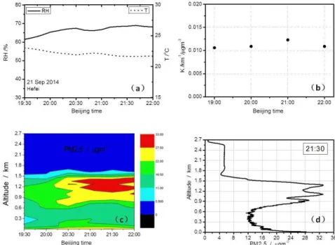
On 21 September 2014, it was clear at night, with northeast wind of not more than 3 m s−1near ground. The temperature ranges from 21.6 to 23.0◦C with a slight decreasing trend, and the RH increases from 61 to 69 % during the time span of 19:30–22:00 Beijing time (BT) as shown in Fig. 3a. The distanceDbetween laser beam and CCD camera is 34.34 m. Figure 3b plots the hourly mean value ofK varying from 0.011 to 0.012 km−1(µg m−3), which indicates an approxi-mately constant value during this experimental case. With the specific coefficientK and the aerosol extinction coefficient profile, PM2.5profile is given accordingly. Fig. 3c presents spatiotemporal distribution of PM2.5mass concentration for this case at the Hefei site. The PM2.5is almost enclosed be-low 1.5 km above ground level (a.g.l.) with a maximum value 33 µg m−3, indicating a clean night in Hefei. The floating layer of 0.6–1.5 km a.g.l. indicates a higher PM2.5, of which the value is more than that below 0.3 km a.g.l. near the Earth surface layer from Fig. 3c. The floating layer exists through-out the night due to a stable aerosol loading. There is a clean layer between the floating layer and the Earth surface layer. It is noted from Fig. 3d that the PM2.5value decreases from 28 µg m−3on the Earth surface to 12 µg m−3at 0.3 km a.g.l., and keeps at a certain value at 0.3–0.6 km a.g.l., and then in-creases to three sub-peaks of 29, 33, and 33 µg m−3 in the floating layer, respectively. The vertical distribution of PM2.5 at 21:30 BT measured at the Hefei site on 21 September 2014 depicts a rich structure.
4.2 Case II: Pollutant night
On 17 March 2014, it was also clear at night, with the south wind of not more than 3 m s−1 near the Earth surface. The temperature varies from 18.2 to 21.7◦C with a decreasing trend and the RH increases from 58 to 70 % during the time span of 19:30–24:00 BT as shown in Fig. 4a. The distanceD
between laser beam and CCD camera is 23.90 m.
Figure 3. (a)RH andT parameters with time,(b)Kvalue for each hour,(c)time series of PM2.5profile, and(d)vertical distribution of PM2.5at 21:30 BT measured at the Hefei site on 21 September 2014.
Figure 4. (a)RH andT parameters with time,(b)Kvalue for each hour,(c)time series of PM2.5profile, and(d)vertical distribution of PM2.5at 21:30 BT measured at the Hefei site on 17 March 2014.
below 1.8 km a.g.l. with a maximum value of 70 µg m−3, in-dicating a mild pollutant night in Hefei. Between 0.6 and 1.8 km a.g.l., the PM2.5value is almost constant, indicating a well-mixed layer. The maximum value of PM2.5lies near the Earth surface layer and forms a rather stable aerosol struc-ture, which will cause a hazy day with poor visibility.
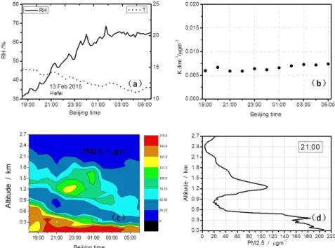
Figure 5. (a)RH andT parameters with time,(b)Kvalue for each hour,(c)time series of PM2.5profile, and(d)vertical distribution of PM2.5at 21:00 BT measured at the Hefei site on 13–14 February 2015.
4.3 Case III: Heavy pollutant night
On 13–14 February 2015, it was also cloud-free at night, with the northwest wind of not more than 3 m s−1 near the ground. The temperature varies from 10.7 to 9.1◦C with a decreasing trend and the RH increases speedily from 31 to 68 % during the time span of 18:30–02:00 BT, and then keeps around 65 % in the late period of 02:00–05:30 BT as shown in Fig. 5a. The distance D between laser beam and CCD camera is 19.40 m.
Figure 5b plots the hourly mean value ofKvarying from 0.006 to 0.007 km−1(µg m−3), which also indicates an ap-proximate constant value during this experimental case. But this value is quite different from that obtained from CASE I and CASE II probably due to the differences in aerosol size distribution and refractive index. The PM2.5 profile is calculated accordingly by the K value and the aerosol ex-tinction coefficient profile. At the meantime, the spatiotem-poral distribution of PM2.5 mass concentration for this case at the Hefei site is shown in Fig. 5c. The PM2.5 rises to 2.1 km a.g.l. with a maximum value 210 µg m−3, indicating a heavy pollutant night in Hefei. During the observation pe-riod, there are three distinct layers (i.e., the floating layer, the clean layer, and the Earth surface layer) with a gradual fall in height from the evening to the next morning. The typical height for the floating layer decreases from 1.2–1.8 to 0.5– 1.0 km a.g.l., and the peak value of PM2.5 for this layer is about 150 µg m−3. The PM2.5value for the fair layer in mid-dle part varies from 30 to 50 µg m−3. The top height of the Earth surface layer decreases from 0.9 km a.g.l. at 18:00 BT
to 0.3 km a.g.l. at 06:00 BT, which leads to a more stable structure. The maximum value of PM2.5 lies near the Earth surface layer, especially below 0.3 km a.g.l., where a high value region of PM2.5(i.e., 200 µg m−3exists all along from 20:00 to 04:00 BT, which will cause a heavy hazy day with worse visibility.
It is noticeable from Fig. 5d that the PM2.5 value takes on a sub-peak of 110 µg m−3 at 1.2 km a.g.l., and increases rapidly from 20 µg m−3 at 0.8 km a.g.l. to another sub-peak of 190 µg m−3 at 0.4 km a.g.l., then increases rapidly again to a peak of 210 µg m−3on the Earth surface. The vertical distribution of PM2.5at 21:00 BT measured at the Hefei site on 13–14 February 2015 forms a more stable and rich struc-ture.
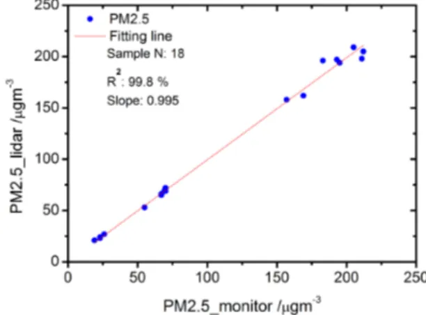
In order to validate the new method mentioned above, the comparison of surface PM2.5 measured by PM2.5 Monitor and C-Lidar is shown in Fig. 6. The values of PM2.5are ob-tained from the foregoing cases and the slope for the fitting line is 0.995 with a correlative coefficient of 99.8 %, which indicates a good agreement. So, the new method is effective to explore PM2.5profile at the near-ground level when RH is less than 70 %.
5 Summary and conclusion
Figure 6.Comparison of surface PM2.5obtained by PM2.5Monitor and C-Lidar.
1. Five types of aerosol from OPAC, prevailing at the Hefei site, are used to testify their extinction coefficient de-pending on RH, only to indicate seldom reliance on RH when RH is less than 70 %.
2. The specific coefficientK, which is related to aerosol size distribution, refractive index, and atmospheric rela-tive humidity, may contain a fixed value under the suit-able condition when RH is less than 70 %, though it may not be the same for each case. So, the PM2.5mass con-centration profile can be easily derived from vertical dis-tribution of extinction coefficient for aerosol.
3. The PM2.5 is always loading in the planet boundary layer with a multi-layered structure, indicating its com-plexity of the vertical distribution. And there is a higher lifting height under the heavy-pollution weather condi-tion, demonstrating that air pollution may break through near the surface into a higher altitude and join in further transportation.
4. The high value of PM2.5 remains near the ground and forms a stable structure, especially on hazy days, which will cause bad weather conditions, such as low visibil-ity.
5. Our new method for PM2.5 mass concentration profile is a useful approach for improving our understanding of air quality and the atmospheric environment, which can also provide critical information for the daily air quality forecast. Further investigation will be carried on in the near future when RH is larger than 70 %, including the potential variation of specific coefficientK.
Acknowledgements. This research is supported by the National Natural Science Foundation of China (Nos. 41175021, 41305022 and 41590870), the Ministry of Science and Technology of China (No. 2013CB955802). We also express our gratitude to
all the anonymous reviewers for their constructive and insightful comments.
Edited by: P. Xie
References
An, J., Zhang, R., and Han, Z.: Seasonal changes of total suspended particles in the air of 15 big cities in northern parts of China, Climatic and Environmental Research, 5, 25–29, 2000.
Bernes, J. E., Bronner, S., and Becket, R.: Boundary layer scattering measurements with a charge-coupled device camera lidar , Appl. Optics, 42, 2647–2652, 2003.
Bo, G., Liu, D., and Wu, D.: Two-wavelength lidar for ob-servation of aerosol optical and hygroscopic properties in fog and haze days, Chinese Journal of Lasers, 41, 0113001, doi:10.3788/cjl201441.0113001, 2014.
Che, H., Xia, X., Zhu, J., Wang, H. Wang, Y., Sun, J., Zhang, X., and Shi, G.: Aerosol optical properties under the condition of heavy haze over an urban site of Beijing, China, Environ. Sci. Pollut. R., 22, 1043–1053, doi:10.1007/s11356-014-3415-5, 2015. Cordero, L., Wu, Y., Gross, B. M., and Moshary, F.: Use of passive
and active ground and satellite remote sensing to monitor fine particulate pollutants on regional scales, Advance environmen-tal, chemical, and Biological sensing technologies IX, Proc. Of SPIE, 8366, 83660M, 2012.
He, X., Deng, Z., Li, C., Lau, A. K., Wang, M., Liu, X., and Mao, J.: Application of MIDIS AOD in surface PM10evaluation, Acta Scientiarum Naturalium Universitatis Pekinensis, 46, 178—184, 2010.
Hess, M., Koepke, P., and Schult, I.: Optical properties of aerosols and clouds: The software package OPAC, B. Am. Meteorol. Soc., 79, 831–844, 1998.
Li, Q., Li, C., Wang, Y., Lin, C., Yang, D., and Li, Y.: Retrieval on mass concentration of urban surface suspended particulate matter with lidar and satellite remote sensing, Acta Scientiarum Natu-ralium Universitatis Pekinensis, 49, 673—682, 2013.
Ma, X.,Tao, Z., and Ma, M.: The retrival of side-scatter lidar sig-nal based on CCD technique, Acta Optica Sinica, 34, 0201001, doi:10.3788/aos201434.0201001, 2014.
Mao, F., Gong, W., and Li, J.: Geometrical form factor calculation using Monte Carlo integration for lidar, Opt. Laser Technonol., 44, 907–912, 2012.
Mao, J., Zhang, J., and Wang, M.: Summary comment on research of atmospheric aerosol in China, Acta Meteorologica Sinica, 60, 625–634, 2002.
Pesch, M. and Oderbolz, D.: Calibrating a ground based backscatter lidar for continuous measurements of PM2.5, lidar technology, techniques, and measurements for atmospheric remote sensing III, Proc. Of SPIE, 6750, 67500K, 2007.
Sano, I., Mukai, M., Okada, Y., Mukai, S., Sugimoto, N., Matsui, I., Shimizu, A.: Improvement of PM2.5analysis by using AOT and lidar data Remote sensing of the atmospheric and clouds U, Proc. Of SPIE, 7152, 71520M, 2008.
Tao, Z., Liu, D., and Wang, Z.: Measurements of aerosol phase function and vertical backscattering coefficient using a charge-coupled device side-scatter lidar, Opt. Express, 22, 1127–1134, doi:10.1364/OE.22.001127, 2014b.
Tao, Z., Liu, D., Ma, X., Shi, B., Shan, H., and Zhao, M.: Verti-cal distribution of near-ground aerosol backscattering coefficient measured by a ccd side-scattering lidar, Appl. Phys. B, 120, 631– 635, 2015.
Wang, Z., Liu, D., Wang, Z., Wang, Y., Khatri, P., Zhou, J., Taka-mura, T., and Shi, G.: Seasonal characteristics of aerosol opti-cal properties at the SKYNET Hefei site (31.90◦N, 117.17◦E) from 2007 to 2013, J. Geophys. Res.-Atmos., 119, 6128–6139, doi:10.1002/2014JD021500, 2014a.
Wang, Z., Liu, D., and Cheng, Z.: Pattern recognition model for haze identification with atmospheric backscatter lidars, Chinese Journal of Lasers, 41, 1113001, doi:10.3788/cjl201441.1113001, 2014b.
Wang, Z., Liu, D., Wang, Y., Wang, Z., and Shi, G.: Diurnal aerosol variations do affect daily averaged radiative forcing under heavy aerosol loading observed in Hefei, China, Atmos. Meas. Tech., 8, 2901–2907, doi:10.5194/amt-8-2901-2015, 2015a.
Wang, Z., Tao, Z., Liu, D., Wu, D., Xie, C., and Wang, Y.: New experimental method for lidar overlap factor using a CCD side-scatter technique, Opt. Lett., 40, 1749–1752, 2015b.
Weitkamp, C.: Lidar: Range-Resolved Optical Remote Sensing of the Atmosphere, Springer, New York, USA, 2005.
Winker, D., Hunt, W., and McGill, M.: Initial performance of assessment of CALIOP, Geophys. Res. Lett., 34, L19803, doi:10.1029/2007GL030135, 2007.
Wu., Z., Liu, A., and Zhang, C.: Vertical distribution feature of PM2.5and effect of boundary layer in Tianjin, Urban Environ-ment & Urban Ecology, 22, 24–29, 2009.
Xu, J., Ding, G., and Yan, P.: Componential characteristics and sources identification of PM2.5 in Beijing, Journal of Applied Meteorological Science, 18, 645–654, 2007.
Yang, L., He, K., and Zhang, Q.: Vertical distributive characters of PM2.5at the ground layer in Autumn and Winter in Beijing, Re-search of Environmental Sciences, 18, 23–28, 2005.