www.atmos-chem-phys.net/15/11165/2015/ doi:10.5194/acp-15-11165-2015
© Author(s) 2015. CC Attribution 3.0 License.
Evaluation of regional background particulate matter concentration
based on vertical distribution characteristics
S. Han1,2, Y. Zhang1, J. Wu1, X. Zhang1, Y. Tian1, Y. Wang1, J. Ding1, W. Yan1, X. Bi1, G. Shi1, Z. Cai2, Q. Yao2, H. Huang2, and Y. Feng1
1State Environmental Protection Key Laboratory of Urban Ambient Air Particulate Matter Pollution Prevention and Control,
College of Environmental Science and Engineering, Nankai University, Tianjin, 300071, China
2Research Institute of Meteorological Science, Tianjin, 300074, China
Correspondence to:Y. Zhang (zhafox@126.com) and Y. Feng (fengyc@nankai.edu.cn) Received: 27 January 2015 – Published in Atmos. Chem. Phys. Discuss.: 27 May 2015 Revised: 15 September 2015 – Accepted: 18 September 2015 – Published: 7 October 2015
Abstract.Heavy regional particulate matter (PM) pollution in China has resulted in an important and urgent need for joint control actions among cities. It is advisable to improve the understanding of the regional background concentration of PM for the development of efficient and effective joint control policies. With the increase of height the influence of source emission on local air quality decreases with alti-tude, but the characteristics of regional pollution gradually become obvious. A method to estimate regional background PM concentration is proposed in this paper, based on the ver-tical characteristics of periodic variation in the atmospheric boundary layer structure and particle mass concentration, as well as the vertical distribution of particle size, chemical composition and pollution source apportionment. According to the method, the averaged regional background PM2.5
con-centration in July, August and September 2009, being ex-tracted from the original time series in Tianjin, was 40±20, 64±17 and 53±11 µg m−3, respectively.
1 Introduction
Atmospheric particulate matter (PM) has attracted consid-erable attention because it has been associated with many urban environmental problems, such as acid precipitation, decreasing visibility and climate change (Zeng and Hopke, 1989; Charlson et al., 1992; Schwartz et al., 1996; Chamei-des et al., 1999). PM has also been implicated in human mor-tality and morbidity (Dockery et al., 1993; Tie et al., 2009; Lagudu et al., 2011). Among the various sizes of atmospheric
PM, PM2.5(PM with aerodynamic diameter less than 2.5 µm)
is considered to be of great significance due to its links to human respiratory health (Englert, 2004), regional-scale air pollution (Husar et al., 1981; Chameides et al., 1999), and potential acid rain enhancement (Cao et al., 2013).
The combination of rapid industrialization and urbaniza-tion has resulted in considerable environmental problems throughout China, especially in the clusters of cities (Shao et al., 2006). The coexistence of numerous air pollutants with high concentrations and the complicated interactions among them leads to the formation of an air pollution complex (Shao et al., 2006; Zhu et al., 2011). One of the major pollutants is PM (Tie et al., 2006; Liu et al., 2011; Chen et al., 2012; Han et al., 2013). The origin of PM is complex. It involves both primary emissions as well as secondary particle produc-tion due to chemical reacproduc-tions in the atmosphere (Shi et al., 2011; Tian et al., 2013; Hu et al., 2013; Guo et al., 2013). With a lifetime of days to weeks in the lower atmosphere, PM2.5 can be transported thousands of kilometres (Hagler
et al., 2006). The trans-boundary transport of PM2.5and the
gaseous precursors has significant influence on the regional background PM level in the cluster of cities. In order to study the regional-scale PM pollution and develop efficient joint control policies, it is necessary to improve understanding of regional background PM concentration.
to-gether with those transported into an airshed from afar (the latter may be either natural or anthropogenic in origin)”. Background concentration in this paper is defined to include collective contributions from regional anthropogenic and nat-ural emissions and long-range transport.
Background concentrations are not constant because of meteorological variability, complexity of chemical reac-tions, as well as spatially and temporally varying emissions. Regional-scale PM pollution is associated with synoptic sce-narios that induce the transfer, accumulation and the forma-tion of pollutants at regional scales. Simply taking measure-ments at local scales is not well suited to adequately investi-gate the regional background concentration. There is always the possibility that the “air quality background monitoring station” is directly influenced by local emission sources and thus not truly representative of the background level (Tche-pel et al., 2010). That is to say, background concentration can hardly be measured directly, so it is critical to choose rep-resentative and appropriate values. Usually, by setting some restrictions to identify and remove the influence of local pol-lution, background concentration can be determined indi-rectly. There are several studies mentioning the methods for determining the background concentration. These methods can be classified into four categories. (1) The physical meth-ods identify the regional pollution process and local pollu-tion process via synoptic situapollu-tion, durapollu-tion of the synoptic system, consistency of vertical wind, atmospheric stability, particle size distribution, etc., and then the data of the “back-ground period” influenced by regional processes are selected (Pérez et al., 2008). (2) The chemical methods identify the regional process according to chemical composition in PM and synchronous observation of other pollutants, and then remove the data influenced by local processes (Menichini et al., 2007). (3) The statistical methods use discriminant analy-sis, cluster analysis and principal component analysis (PCA) to identify the data that characterize the regional background PM (Langford et al., 2009; Tchepel et al., 2010). (4) Nu-merical simulation methods use trajectory models and atmo-spheric dynamics–chemical coupled models to simulate the regional background pollution (Dreyer and Ebinghaus, 2009; Tchepel et al., 2010).
With the increase of height, the influence of source emis-sion on local air quality decreases with altitude, but the characteristics of regional pollution gradually become ob-vious. Influenced by atmospheric dynamics and thermal ef-fects, meteorological variables and pollutant measurements at different heights within the boundary layer could repre-sent different horizontal scales of pollution. Sites at near-ground height (5–10 m) are influenced extensively by human activities, and the data observed at these sites could represent the street scale. Impacts from local disturbance weaken with height gradually and observations at greater heights could represent larger horizontal scales. When the height increases to the top of the urban atmospheric boundary layer, obser-vations can represent urban scales. Heights above the urban
boundary layer could to some extent reflect the character-istics of regional scales. A tall tower is commonly used in observation of boundary layer meteorological, micrometeo-rological and atmospheric chemical variables, e.g. vertical profile and fluxes (Heintzenberg et al., 2008, 2013; Brown et al., 2013; Andreae et al., 2015). The footprint concept is capable of linking observed data collected at the differ-ent height levels of the tower to spatial context. The inte-gral beneath the footprint function expresses the total surface influence on the signal measured by the sensor at a height above the surface (Schmid, 2002; Ding et al., 2005; Foken and Nappo, 2008). Three main factors affect the size and shape of flux footprint: increase in measurement height, de-crease in surface roughness, and change in atmospheric sta-bility from unstable to stable leading to an increase in size of the footprint (https://en.wikipedia.org/wiki/Flux_footprint). Combined information from meteorological data and simul-taneous aerosol measurements at the different levels of the tower have made it possible to gain insights into the transport of aerosols and their vertical distributions which strongly de-pend on meteorological conditions, boundary layer dynam-ics and physiochemical processes (Guinot et al., 2006; Pal et al., 2014). In this paper, the periodic variation in the at-mospheric boundary layer structure and PM mass concen-trations, as well as the vertical distribution characteristics of particle size, chemical composition and pollution sources, were studied to characterize the regional pollution contribu-tion. On this basis, the height above which there is relatively less influence by local pollution emission can be determined and the regional background PM concentration can be ex-tracted from the observation data and estimated by mathe-matical methods.
2 Data sources and treatment 2.1 Observation site
The data used in this study were collected at a 255 m meteorological tower which is located at the atmospheric boundary layer observation station (WMO Id. No. 54517, 39◦04′29.4′′N, 117◦12′20.1′′E) in Tianjin, China, where there is a residential and traffic mixing area. There are no in-dustrial pollution sources near the site. Tianjin is adjacent to the BoHai Sea and situated in the eastern part of the Beijing– Tianjin–Hebei area, one of the most heavily polluted areas in China. Tianjin covers an area of 11 300 km2and has a
pop-ulation of 8 million. Due to rapid industrialization and ur-banization in recent years, air pollution has become a serious problem in this city.
2.2 Observation method and data treatment
averaged hourly. Three-dimensional ultrasonic anemometers (CAST-3D) were mounted at 40, 120 and 220 m to measure the turbulent fluxes. Hourly meteorological data (WMO Id. No. 54517) in the year of 2009 were used in this paper.
Mass concentrations of PM2.5 were measured using
ambient particulate monitor chemiluminescence (TEOMR-RP1400a) at four different heights (2, 40, 120, and 220 m) from 1 July to 30 September 2009. The monitor’s data out-put consists of 1 and 24 h average mass concentration up-dated every 10 min and on the hour, with the precision of
±1.5 µg m−3 (1 h avg) and
±0.5 µg m−3 (24 h avg)
respec-tively. The accuracy of mass measurement is±0.75 %. In order to study the vertical characteristics of PM chem-ical composition and sources, 24 h PM10 filter samples were
collected from local Beijing time 08:00 to 07:00 GMT+8:00 the next day using medium-volume PM10 samplers
(TH-150, Wuhan Tianhong Intelligence Instrumentation Facility) at the heights of 10, 40, 120, and 220 m from 24 August to 12 September 2009. The sampler has a system of automatic constant-flow control. Flow rate of sampling in this study is 100 L min−1, and the relative error of flow is less than 3 %.
At each height, PM10 filter samplings were equipped with
two samplers in parallel: one is for chemical analysis of inor-ganic composition on polypropylene filters (90 mm in diam-eter, Beijing Synthetic Fiber Research Institute, China) and the other is for organic composition analyses on quartz-fibre filters (90 mm in diameter, 2500QAT-UP, Pall Life Sciences). Before and after sampling, filters were conditioned for 48 h in darkened desiccators prior to gravimetric determina-tion. The filters were weighed on a electronic microbalance (AX205, Mettler-Toledo, LLC, with a±0.01 mg sensitivity) in a clean room under constant temperature (20±1◦) and RH (40±3 %). Samples were stored air-tight in a refrigerator at about 4◦before chemical analyses.
Elements (Si, Ti, Al, Mn, Ca, Mg, Na, K, Cu, Zn, Pb, Cr, Ni, Co, Fe, and V) were analysed by Inductively Coupled Plasma atomic emission spectroscopy (ICP 9000 (N+M) Thermo Electron Corporation, USA). Blank filters were pro-cessed simultaneously with sample filters. Ultrapure water, both unfiltered and filtered, and nitric acid were also anal-ysed. The average element values in the blanks were sub-tracted from those obtained for each sample filter; 10 % of total samples were analysed in duplicate to verify sample homogeneity. The precision and accuracy were checked by analysis of an intermediate calibration solution. Extraction efficiencies were evaluated by analysis of the certified refer-ence material from the National Research Center for CRM. The recovery value was between 85 and 110 %. Calibration check was performed to ensure a relative error of no more than 2 % for major elements and 5 % for trace elements.
Water-soluble ions (NH+
4, Cl−, NO−3, and SO24−) were
analysed by ion chromatography (DX-120, Dionex Ltd., USA) after extraction by deionized water. External calibra-tion was employed to quantify the ion concentracalibra-tions. A cal-ibration check with external standards was performed to
en-sure a relative error of no more than 10 %. The uncertainty contributions of the calibration curve, calibration solution and repetitive measurement for unknown sample were taken into account. The expanded uncertainty was 3.8 % with a coverage factor ofk=2.
The thermal optical carbon analyser (Desert Research In-stitute (DRI) Model 2001, Atmoslytic Inc., Calabasas, CA, USA) was used to measure organic carbon (OC) and ele-mental carbon (EC). The heating process can be found in the IMPROVE_A protocol (Chow et al., 2010, 2011; Cao et al., 2003). Field blank and lab blank were considered and all sampling concentrations were revised by blank concentra-tion. The uncertainty contributions of the calibration curve, calibration solution and repetitive measurement for unknown sample were taken into account. The expanded uncertainty was 7.6 % with a coverage factor ofk=2.
3 Vertical variation characteristics of urban boundary structure
3.1 Thermal and dynamic characteristics in surface layer
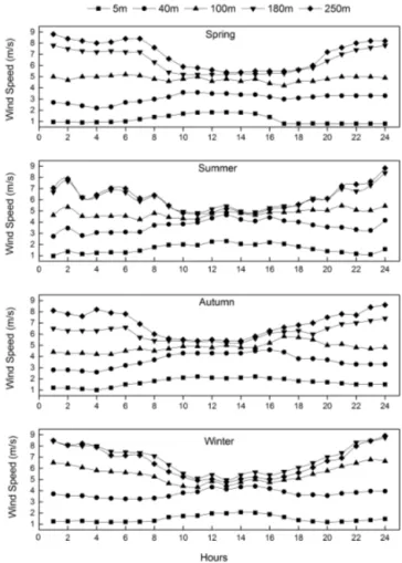
Surface layer has a remarkable effect on the diffusion of air pollutants. This layer is strongly affected by human be-haviour on the ground. Figure 1 presents the diurnal variation of averaged wind speed in four seasons at different heights in Tianjin. The four seasons were designated as March–May for spring, June–August for summer, September–November for autumn, and December–February for winter. Diurnal varia-tion patterns of wind speed were similar in each season. The wind speed is high in daytime and low at night below 100 m, whereas there is low wind speed in the daytime and high wind speed at night above 100 m.
Figure 2 shows the vertical profile of wind speed and tem-perature in low atmosphere under different stability. The gra-dient Richardson number (Ri) was used for classifying the atmospheric stability conditions:
Ri= g
T
"
1T √z
1z2lnzz21 +rd
#
×
"√
z1z2lnzz21 1u
#
, (1)
where1T =T2−T1,1u=u2−u1,T2andT1are the
mea-sured temperatures at the height ofz2andz1,T is the
av-eraged temperature in the layer between levelz2andz1,u2
andu1are the measured wind speed at levels z2 andz1,g
is the gravitational acceleration, andrd is the dry adiabatic
lapse rate. According to the values ofRi, three different con-ditions can be distinguished: Ri≥0.1 for stable condition,
−0.1<Ri<0.1 for neutral condition, andRi≤ −0.1 for un-stable condition.
tem-Figure 1.Diurnal variation of averaged wind speed in each season at different heights.
perature profile was observed over 100 m. Similarly, a small vertical gradient in wind speed was found over 150 m. 3.2 The height of nocturnal planetary boundary and
vertical variation of turbulent intensity
The height of the planetary boundary layer (PBL), indicating the range of pollutants diffused by thermal turbulence in the vertical direction (Kim et al., 2007; Lena and Desiato, 1999), can be calculated by wind and temperature profiles (Seibert et al., 2000; Han et al., 2009). Based on the temperature pro-file observed at the tower, the vertical gradient of temperature was calculated as
1T
1Z =
T (z+1)−T (z)
Z (z+1)−Z (z), (2)
whereT (z+1)andT (z)represent the measured tempera-tures at levelsz+1 andz, andZ (z+1)andZ (z)represent the altitudes at levelsz+1 andz. The height of the nocturnal planetary boundary layer (NPBL) is determined by the bot-tom of the inversion, i.e. the layer in which the temperature profile has a positive gradient. As shown in Fig. 3, the
sea-Figure 2.Vertical distribution profile of average wind speed and temperature in low atmosphere under different stability conditions.
sonal variation of the NPBL height is generally small, with seasonal averaged NPBL height ranging from 114 to 142 m. In this study, hourly averaged PM2.5 concentration
mea-surement and 24 h PM10 filter sampling were conducted at
four platforms. The heights of the first and second platform are inside the NPBL, the third platform is located at the top of the NPBL, and the fourth platform is generally outside the NPBL. Due to the dynamical stability of the NPBL, air pollutants in the surface layer are normally trapped inside the NPBL and rarely mix with the pollutants outside the NPBL. Very different distribution characterizations of PM were measured inside and outside the NPBL (see Sect. 4).
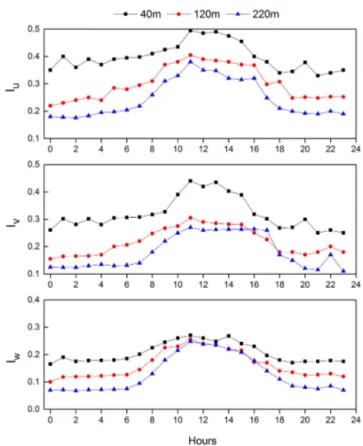
Based on the observation data from the three-dimensional ultrasonic anemometers, the turbulent intensity were calcu-lated. As a whole, the averaged diurnal variations of turbulent intensity in each season (Fig. S1 in the Supplement) were re-flecting the same trends. The diurnal peaks appeared later and turbulent intensity was slightly weaker in winter than in other seasons. Averaged diurnal variation of turbulent inten-sity at different heights during the year of 2009 is shown in Fig. 4. Three-dimensional components of turbulent intensity decreased with increase in height. From the height of 40 to 120 m, theu,v andwcomponents of turbulent intensity
re-duced by 27, 32 and 21 %, respectively. From 120 to 220 m, theu,vandwcomponents reduced by 12, 13 and 15 %, re-spectively. The descending trend is more obvious from 40 to 120 m than from 120 to 220 m. This indicates that there were full vertical and horizontal turbulence exchanges be-low 120 m of the tower, but relatively weaker exchanges over 120 m.
4 Vertical distribution of PM2.5mass concentration The diurnal variation of PM2.5 mass concentrations during
the period from 1 July to 30 September 2009 is shown in Fig. 5. The vertical variation patterns of PM2.5
re-Figure 3. Averaged NPBL height in each season (before dawn 01:00–07:00; at night: 19:00–24:00 GMT+8:00).
sulting from a combination of diurnal variations of emissions and PBL. After sunrise, the PBL height starts to rapidly in-crease, pollutants near the ground gradually diffuse upward and the PM2.5concentration near the surface gradually
de-creases. At noon, the mixing layer is fully developed with the averaged PBL height being about 1000–1200 m. Among these four platforms (2, 40, 120 and 220 m), PM2.5
concen-tration at 220 m is the highest during noon and afternoon. In contrast, after 18:00 GMT+8:00, the PBL height starts to rapidly decrease. The NPBL height generally ranges be-tween 100 and 150 m (Fig. 3). At the first and second plat-form (2, 40 m), the measured PM are normally inside of the NPBL. By contrast, the measurement platform at 220 m is generally outside the NPBL. Level 3 (120 m) is considered as being at the transition zone between the inside and outside of the NPBL. Due to the dynamical stability of the NPBL, the vertical mixing of pollutants between inside and outside of the NPBL is very weak. The surface emitted PM are nor-mally trapped inside the NPBL, leading to the difference in the amount of aerosols below and above the NPBL. Among these four platforms, PM2.5 concentration at 220 m during
the night is the lowest. This indicates that the observation value of 220 m at night is less affected by local sources of emission and is largely attributed to regional-scale pollution.
5 Vertical distributions of PM10concentration, composition and source apportionment
5.1 Vertical characteristics of PM10concentration As mentioned in Sect. 2.2, PM10 filter samples were
col-lected at the heights of 10, 40, 120 and 220 m. The daily con-centrations at each sampling height were 139±45, 121±43, 110±39 and 79±37 µg m−3, respectively. These
concentra-tions exhibited a general decreasing trend with the increase of height.
Figure 4.Averaged diurnal variation of three-dimensional compo-nents of turbulent intensity at different heights (longitudinal turbu-lent intensityIu, lateral turbulent intensityIv, vertical turbulent
in-tensityIw).
The height-to-height correlation coefficients of the varia-tion of PM10concentration were calculated and listed in
Ta-ble 1. All the pairwise correlation coefficients among 10, 40 and 120 m were higher than 0.9. However, the correlation co-efficients between 220 m and other heights were obviously low. These results suggest that the influences of local emis-sions and local meteorological diffusion conditions on PM10
concentrations are weaker at 220 m than at lower levels. 5.2 Vertical characteristics of PM10chemical
composition
Coefficient of divergence (CD) analysis (Wongphatarakul et al., 1998; Krudysz et al., 2009) was used in this study to as-sess vertical variability of chemical elements in PM10 filter
samples collected at four heights. The CD values provide information on the degree of uniformity between sampling sites and is defined as
CDj k=
v u u t 1
p
p
X
i=1
x
ij−xik
xij+xik
2
, (3)
wherexij is the average concentration of theith element at
Figure 5.Vertical diurnal variation of PM2.5mass concentrations
during the period from 1 July to 30 September 2009.
andpis the number of elements. When the species concen-trations at two sampling sites were similar to each other, the CD values would approach 0. On the other hand, as the two species concentrations diverge the CD value will approach 1 (Hwang et al., 2008).
The pair-wise CD values for four heights are shown in Ta-ble 2. The pair-wise CD values among 10, 40 and 120 m are lower than 0.2, illustrating that the element profiles of these three heights were similar to each other, while the CD val-ues between 220 m and the other three levels were obviously high. This may have resulted from the fact that chemical el-ements in the PM10 filter samples collected at 220 m were
mainly originated from regional-scale sources.
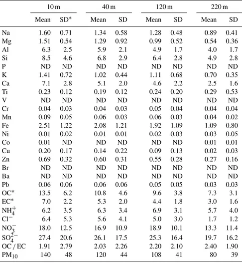
The concentration of chemical composition in ambient PM10filter samples collected at four heights are shown in
Ta-ble 3. Al, Si, Ca, OC, EC, Cl−, NO−
3 and SO24−have higher
concentration levels than other species. Al can be used as a source marker of coal combustion (Hopke, 1985); Al and Si are the markers of soil dust (Liu et al., 2003), Ca is mainly emitted from cement dust (Shi et al., 2009); EC can be iden-tified as vehicle exhaust emission (Li et al., 2004); Cl− is the marker for sea salt (Li et al., 2004); and NO−
3 and SO24−
are the markers of secondary nitrate and sulfate (Liu et al., 2003). Higher concentrations were found at lower sampling heights for almost all species (NO−
3 had the highest value at
120 m). Unlike the species concentration, the vertical distri-bution of species percentages (%) shows different patterns. Similar fraction levels were observed at the four heights for Al and Si. For Ca and EC, higher values were observed at lower sampling sites. The percentages of OC at 220 m were obviously higher than those at 120 m. This might imply that the influence of local sources on OC was weaker and the con-tributions from secondary and regional sources were larger at 220 m. The OC/EC ratios increased gradually from 10 to 220 m. This might be due to a relatively higher percentage of SOC in OC at higher heights as a result of the formation and regional transport of SOC (Strader et al., 1999). Simi-larly, the higher sampling sites obtained higher fractions (%)
Table 1.Height-to-height correlation coefficient of PM10 concen-tration.
10 m 40 m 120 m 220 m
10 m 1.0 40 m 0.96 1.0
120 m 0.91 0.94 1.0 220 m 0.72 0.76 0.85 1.0
Table 2.Pair-wise CD values at different heights.
10 m 40 m 120 m
40 m 0.10 120 m 0.15 0.11
220 m 0.33 0.30 0.59
for NO−
3 and SO24−(the highest percentage of NO−3 was
ob-served at 120 m). These trends suggest that the impact of pri-mary sources from the ground decreased with the increase of height, while the impact of secondary sources mainly influ-enced by regional sources becomes more prominent. 5.3 Vertical characteristics of PM10sources
In order to understand the vertical characteristics of PM10
sources, the chemical mass balance (CMB) model was ap-plied for source apportionment at all four sampling heights. The CMB model, a useful receptor model, has been exten-sively used to estimate source categories and contributions to the receptor based on the balance between sources and the receptor (Chow et al., 2007; Watson et al., 2008). Further de-tails of CMB can be found in the relative literature (Watson et al., 1984, 2002; USEPA, 2004). The data set of chemical composition in the PM10 samples during the measurement
period and the source profiles reported in our previous works (Bi et al., 2007) were used in the CMB modelling.
Six source categories (coal combustion, crustal dust, ce-ment dust, vehicle exhaust, secondary sulfate and secondary nitrate) and their source contributions (µg m−3)and
percent-age contributions (%) estimated by the CMB model are listed in Table 4. The estimated source contributions (µg m−3)of
Table 3.The concentration of chemical composition in ambient PM10at four height sampling sites (µg m−3).
10 m 40 m 120 m 220 m
Mean SD∗ Mean SD Mean SD Mean SD
Na 1.60 0.71 1.34 0.58 1.28 0.48 0.89 0.41 Mg 1.51 0.54 1.29 0.92 0.99 0.52 0.54 0.36 Al 6.3 2.5 5.9 2.1 4.9 1.7 4.0 1.7 Si 8.5 4.6 6.8 2.9 6.4 2.8 4.9 2.8 P ND ND ND ND ND ND ND ND K 1.41 0.72 1.02 0.44 1.11 0.68 0.70 0.35 Ca 7.1 2.8 5.1 2.0 4.6 2.2 2.5 1.6 Ti 0.23 0.12 0.19 0.12 0.24 0.20 0.29 0.53 V ND ND ND ND ND ND ND ND Cr 0.04 0.03 0.04 0.03 0.05 0.04 0.04 0.04 Mn 0.09 0.05 0.06 0.03 0.06 0.03 0.04 0.02 Fe 2.51 1.22 2.08 1.21 1.92 1.09 1.09 0.80 Ni 0.01 0.02 0.01 0.01 0.02 0.03 0.03 0.05 Co 0.01 ND ND ND ND ND 0.01 0.01 Cu 0.20 0.17 0.14 0.22 0.09 0.13 0.02 0.03 Zn 0.69 0.32 0.60 0.31 0.55 0.28 0.27 0.16 Br ND ND ND ND ND ND ND ND Ba ND ND ND ND ND ND ND ND Pb 0.06 0.06 0.06 0.06 0.05 0.05 0.03 0.03 OC∗ 13.5 6.2 10.8 4.6 9.6 3.8 7.3 3.1 EC∗ 7.0 2.2 5.3 2.0 4.4 1.8 3.0 1.6 NH+
4 6.2 3.5 6.3 3.4 6.9 3.1 5.7 4.0
Cl− 6.4 5.3 5.6 4.1 5.0 3.0 1.7 1.2 NO−
3 18.0 12.5 16.9 10.9 18.9 10.1 13.3 11.4
SO2−
4 27.4 20.6 26.1 17.5 25.3 16.4 19.7 16.2
OC/EC 1.91 2.79 2.03 2.26 2.20 2.10 2.40 1.90 PM10 140 48 120 44 108 41 80 39
∗SD: standard deviation; OC: organic carbon; EC: element carbon.
6 Vertical variation of periodicity for the time series of PM2.5concentrations
The periodic characteristics of particulate concentration and meteorological variables can reflect different scales of atmo-spheric processes. In this paper, the vertical variation period of PM2.5mass concentrations are analysed.
A time series of atmospheric pollutant concentration can be decomposed into baseline and short-term components. Using the filtering method, short-term fluctuations associ-ated with the influence of local-scale pollution and dispersion conditions can be extracted from the original measurements. After the removal of local-scale effects, the time series of pollutant concentrations can be reconstructed to reflect the regional-scale influence.
6.1 Filtering method
The wavelet transform can be used to analyse time series that contain nonstationary signals at many different frequencies. In this paper, we chose the Morlet wavelet which is exten-sively used in studies of climate change and turbulence power
spectrum analysis (Torrence and Compo, 1998). The normal-ization mother wavelet is
ψ0(η)=π−1/4eiω0ηe−η 2/2
, (4)
where η is the nondimensional time parameter and ω0 is
the nondimensional frequency. The wavelet filter time series over a set of scales can be calculated by
xn=
δj δt1/2 Cδψ0(0)
J
X
j=0
RWn sj
sj1/2
, (5)
whereδj is the spacing between the discrete scales, andδt
is the sampling interval.Sj is a set of scales related to the
frequencyω.Cδandψ0(0)are both constants:
ω=
ω0+
q 2+ω20
4π s . (6)
Table 4.Source contributions and percentage contributions at four different heights.
Coal Crustal Cement Vehicle Secondary Secondary TOT combustion dust dust exhaust sulfate nitrate
Contribution 10 m 17 16 14 20 34 23 140 (µg m−3) 40 m 16 13 10 17 33 21 120
120 m 14 12 8 15 32 24 108 220 m 12 9 4 12 25 17 80
Percentage 10 m 12 11 10 14 24 16 88 (%) 40 m 13 11 8 14 27 18 90 120 m 13 11 8 14 29 22 97 220 m 14 11 5 15 31 21 97
Table 5.Values of the parameters of the Morlet transform in this study.
Cδ ψ0 s0 δt δj ω0
0.776 π−1/4 2δt 2 0.25 6.0
Cδ=
δj δt1/2 ψ0(0)
J
X
j=0
RWδ sj
sj1/2
. (7)
According to the conservation of total energy under the wavelet transform and the equivalent of Parseval’s theorem for wavelet analysis, the variance of the time series is
σ2= δj δt CδN
N−1
X
n=0
J
X
j=0
Wn sj
2
sj
. (8)
Both Eqs. (7) and (8) should be used to check wavelet rou-tines for accuracy and to ensure that sufficiently small values ofs0andδj have been chosen. The values of the above
pa-rameters are given in Table 5.
As discussed above, the wavelet transform is essentially a bandpass filter. By summing over a subset of the scales in Eq. (5), a wavelet-filtered time series can be constructed as follows:
xn′ = δj δt 1/2 Cδψ0(0)
j2
X
j=j1
RWn sj
sj1/2
. (9)
This filter has a response function given by the sum of the wavelet functions between scalej1andj2.
6.2 Fluctuation spectrum analysis of PM2.5 concentration time series at different heights The fluctuation spectrum distribution of hourly mass con-centrations of PM2.5 on the ground and at the height of 2,
40, 120 and 220 m have been analysed in this paper. Miss-ing data in the time series were computed by interpolation.
Because of low proportions and unconcentrated distributions in the missing data, little human interference was applied to the spectral composition of the original time series. For bet-ter comparison, normalization (standard variance 1, mean 0) of the original time series was necessary prior to power spec-trum analysis.
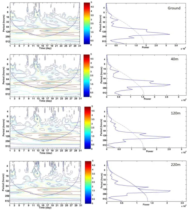
The local and global wavelet power spectrum contours for the time series of PM2.5concentrations at different heights
in August are shown in Fig. 6. Contours are expressed as log2 |Wn(s)|2
because of large magnitudes. The area inside the thick black solid line passes the red noise standard spec-tral test with the 5 % significance level. The area outside the blue dotted line was excluded from analysis because of poor reliability from the cone of influence, where edge effects be-come important. The global wavelet spectrumW2(s), which reflects characteristics of the pollutant concentration time se-ries in the frequency domain, was obtained by calculating the average of local wavelet spectra|Wn(s)|2over the entire
sampling time domain. The solid line is the global wave spec-trum for the corresponding time series. The dashed line is the 5 % significance level, the upper area of which passes the red noise standard spectral test at the 5 % significance level.
The global wavelet power spectrum of PM2.5mass
con-centration shows that fluctuations of 6–10 days (related to weather process and regional-scale pollution) are significant at each observation height, while fluctuations of 12–24 h (mainly concerned with the daily variation of atmospheric boundary layer and local pollution emissions by human ac-tivities) are significant only at ground level. For the fluctua-tions of PM2.5mass concentration, wave energy of 6–10-day
Figure 6.Local (left panels) and global (right panels) wavelet power spectrum of PM2.5mass concentration at different heights in
Au-gust 2009.
7 Determination of regional background concentration of particulate matter
Regional PM background concentration can hardly be sured directly. Original PM concentration time series mea-sured on the ground reflect a combination of influence from local pollution and regional-scale pollution. This study is ex-pected to establish an approach to characterize the regional pollution contribution and to evaluate regional background PM concentration levels. According to the above research concerning the vertical distribution characteristics of parti-cle size, chemical composition and pollution sources, the at-mospheric boundary layer structure, as well as the
fluctu-ation power spectrum analysis of particle mass concentra-tion, the measurement height (influenced relatively less by local pollution emission) was determined and impacts from local-scale pollution on the short-term fluctuations removed from the original PM concentration by wavelet transforma-tion. The nocturnal PM2.5 mass concentration time series
with the 6–10-day period at the observation height of 220 m was extracted to characterize the regional background con-centration, which is mainly associated with the regional-scale pollution within 102km of the measurement tower.
Time series of PM2.5hourly concentration before and
Figure 7.Time series of PM2.5hourly concentration before and after filtering.
observation errors etc., the original PM2.5concentration time
series exhibits a violent oscillation. Using wavelet transfor-mation, the nocturnal PM2.5mass concentration time series
with the 6–10-day period at the height of 220 m was extracted from the original time series. After the filtering, impacts from local-scale pollution and diffusion conditions on the short-term fluctuations were considered to be removed. Thus regional-scale pollution and synoptic-scale weather condi-tions were better represented in the remaining part compared with the original PM concentration time series.
The swings in the PM2.5 concentration data (shown in
Fig. 7) mainly resulted from several meteorological pro-cesses during the measurement. According to the mete-orological data set of the observation station (WMO Id. No. 54517), precipitation processes were recorded during the period of 22–24 July, with the amounts of rainfall ranging from 3.2 to 94.6 mm, followed by a rapid decrease in PM2.5
concentration on 25 July due to consequent cleaning of the air. Then, beginning on 26 July, mist paired with calm winds caused a build-up of PM2.5concentration until 29 July.
Simi-lar meteorological processes were reported during the period of 22–25 August, 4–9 and 20–25 September, which resulted in the cycle of cleaning and build-up of air pollutants.
According to the method proposed in this paper, in Tianjin, the averaged regional background PM2.5 concentrations in
July, August and September 2009 were 40±20, 64±17 and 53±11 µg m−3, respectively.
8 Summary and conclusions
Based on a 255 m meteorological tower, the vertical ther-modynamic and dynamic characteristics of the atmospheric boundary layer in Tianjin was observed. The atmospheric layer at 100–150 m is considered as a transition layer, the variation patterns of temperature and wind speed with height were different compared with the upper and lower layers. A weak vertical gradient in the temperature profile was ob-served over 100 m. Similarly, a small vertical gradient in wind speed was found over 150 m. The turbulent intensity decreased with increase in height and the descending trend is more obvious from 40 to 120 m than from 120 to 220 m, which indicates that there were full vertical and horizontal turbulence exchanges below 120 m of the tower, but rela-tively weaker exchanges over 120 m. Seasonal averaged noc-turnal planetary boundary layer height ranged from 114 to 142 m. The observation height of 220 m is just outside the NPBL, which indicates that the observation value of PM con-centration at 220 m at night is less affected by local primary sources near the ground and is largely the result of regional-scale pollution.
The vertical distribution of chemical composition in PM10
filter samples also suggests that the impact of primary sources near the ground decreased with height, whereas the impact of secondary sources mainly influenced by regional sources became more prominent. The vertical distribution of percentage was different for various species. Similar per-centage levels were observed at the four different heights for Al and Si. For the Ca and EC fractions, higher values were observed at lower sampling sites. The percentages of NO−
3, SO24− and OC, and the OC/EC ratios were
obvi-ously higher at higher sites. Source apportionment for am-bient PM10showed that the percentage contributions of
sec-ondary sources obviously increased with height, while the contribution of cement dust decreased with height. PM at higher height obtained more regional contributions, and to some extent it could reflect the characteristics of the regional scale.
The periodic characteristics of PM2.5mass concentration
can reflect different scales of atmospheric processes. In terms of the global wavelet power spectrum of PM2.5 mass
con-centration, fluctuations of 6–10 days, related to weather pro-cesses and regional-scale pollution, were significant at each observation height, while fluctuations with 12–24 h period, mainly concerned with the daily variation of atmospheric boundary layer and local pollution emissions by human ac-tivities in the surface layer, were significant only at ground level. In terms of the local power spectrum, a 12–24 h period can be observed in a few days on the ground. But with the increase of height, the power of the 12–24 h period became weaker – only 10–30 % of that on the ground.
According to the above research, the nocturnal PM2.5
mass concentration time series with the 6–10-day period at the measurement height of 220 m can be regarded as re-gional background concentration, mainly associated with the regional-scale pollution within 102km of the measurement
tower. Using wavelet transformation and filtering, the noctur-nal PM2.5mass concentration time series with the 6–10-day
period at the height of 220 m was extracted from the origi-nal time series. After removing the impacts from local-scale pollution and diffusion conditions on the short-term fluctu-ations, regional-scale pollution and synoptic-scale weather conditions were better represented in the remaining part com-pared with the original PM concentration time series. Ac-cording to the method proposed in this paper, in Tianjin, the averaged regional background PM2.5 concentrations in
July, August and September 2009 were 40±20, 64±17 and 53±11 µg m−3, respectively.
We have put forward a new method to estimate the regional background concentration of PM. Background PM concen-trations are not constant but vary with space and time. In fu-ture research, more analysis on the characteristics of the ur-ban boundary layer, vertical distribution of PM composition and source apportionment in different seasons and meteoro-logical conditions will be done, and background concentra-tion ranges of PM2.5for given time periods and
meteorolog-ical conditions will be obtained.
The Supplement related to this article is available online at doi:10.5194/acp-15-11165-2015-supplement.
Acknowledgements. This work was funded by the Tianjin Sci-ence and Technology Projects (14JCYBJC22200), the SciSci-ence and Technology Support Program (13ZCZDSF02100), and the National Natural Science Foundation of China (NSFC) under Grant No. 41205089 and No. 21207069. We also thank LetPub (www.letpub.com) for linguistic assistance during the preparation of the manuscript.
Edited by: M. Shao
References
measurements, Atmos. Chem. Phys. Discuss., 15, 11599–11726, doi:10.5194/acpd-15-11599-2015, 2015.
Bi, X., Feng, Y., Wu, J., Wang, Y., and Zhu, T.: Source apportion-ment of PM10in six cities of northern China, Atmos. Environ.,
41, 903–912, 2007.
Brown, S. S., Thornton, J. A., Keene, W. C., Pszenny, A. A. P., Sive, B. C., Dubé, W. P., Wagner, N. L., Young, C. J., Riedel, T. P., Roberts, J. M., VandenBoer, T. C., Bahreini, R., Öztürk, F., Middlebrook, A. M., Kim, S., Hübler, G., and Wolfe, D. E.: Nitrogen, Aerosol Composition, and Halogens on a Tall Tower (NACHTT): Overview of a wintertime air chemistry field study in the front range urban corridor of Colorado, J. Geophys. Res., 118, 8067–8085, doi:10.1002/jgrd.50537, 2013.
Cao, J. J., Lee, S. C., Ho, K. F., Zhang, X. Y., Zou, S. C., Fung, K., Chow, J. C., and Watson, J. G.: Characteristics of carbonaceous aerosol in Pearl River Delta Region, China during 2001 winter period, Atmos. Environ., 37, 1451–1460, 2003.
Cao, J. J., Tie, X. X., Dabberdt, W. F., Tang, J., Zhao, Z. Z., An, Z. S., Shen, Z. X., and Feng, Y. C.: On the potential high acid deposition in northeastern China, J. Geophys. Res., 118, 4834– 4846, doi:10.1002/jgrd.50381, 2013.
Chameides, W. L., Yu, H., Liu, S. C., Bergin, M., Zhou, X., Mearns, L., Wang, G., Kiang, C. S., Saylor, R. D., Luo, C., Huang, Y., Steiner, A.,and Giorgi, F.: Case study of the effects of atmo-spheric aerosols and regional haze on agriculture: an opportu-nity to enhance crop yields in China through emission controls, P. Natl. Acad. Sci., 96, 13626–13633, 1999.
Charlson, R. J., Schwartz, S. E., Hales, J. M., Cess, R. D., Coakley Jr., J. A., Hansen, J. E., and Hofmann, D. J.: Climate forcing by anthropogenic aerosols, Science, 255, 423–430, 1992.
Chen, J., Zhao, C. S., Ma, N., Liu, P. F., Göbel, T., Hallbauer, E., Deng, Z. Z., Ran, L., Xu, W. Y., Liang, Z., Liu, H. J., Yan, P., Zhou, X. J., and Wiedensohler, A.: A parameterization of low visibilities for hazy days in the North China Plain, Atmos. Chem. Phys., 12, 4935–4950, doi:10.5194/acp-12-4935-2012, 2012. Chow, J. C., Watson, J. G., Lowenthal, D. H., Chen, L. W. A.,
Zielinska, B., Mazzoleni, L. R., and Magliano, K. L.: Evalua-tion of organic markers for chemical mass balance source appor-tionment at the Fresno Supersite, Atmos. Chem. Phys., 7, 1741– 1754, doi:10.5194/acp-7-1741-2007, 2007.
Chow, J. C., Watson, J. G., Chen, L.-W. A., Rice, J., and Frank, N. H.: Quantification of PM2.5 organic carbon sampling arti-facts in US networks, Atmos. Chem. Phys., 10, 5223–5239, doi:10.5194/acp-10-5223-2010, 2010.
Chow, J. C., Watson, J. G., Robles, J., Wang, X. L., Chen, L. W. A., Trimble, D. L., Kohl, S. D., Tropp, R. J., and Fung, K. K.: Qual-ity assurance and qualQual-ity control for thermal/optical analysis of aerosol samples for organic and elemental carbon, Anal. Bioanal. Chem., 401, 3141–3152, doi:10.1007/s00216-011-5103-3, 2011. Ding, G., Chen, Z., Gao, Z., Yao, W., Li, Y., Cheng, X., Meng, Z., Yu, H., Wong, K., Wang, S., and Miao, Q.: The vertical struc-ture and its dynamic characteristics of PM10and PM2.5in lower
atmosphere in Beijing city, Sci. China Ser. D, 35, 31–44, 2005. Dockery, D. W., Pope, C. A., Xu, X. P., Spengler, J. D., Ware, J. H.,
Fay, M. E., Ferris Jr., B. G., and Speizer, F. E.: An association between air pollution and mortality in 6 United States cities, N. Engl. J. Med., 329, 1753–1759, 1993.
Dreyer, A. and Ebinghaus, R.: Poly fluorinated compounds in am-bient air from ship- and land-based measurements in northern Germany, Atmos. Environ., 43, 1527–1535, 2009.
Englert, N.: Fine particles and human health-a review of epidemio-logical studies, Toxicol. Lett., 149, 235–242, 2004.
Foken, T. and Nappo, C. J.: Micrometeorology, Springer, Berlin, 308 pp., 2008.
Gu, J. X., Bai, Z. P., Li, W. F., Wu, L. P., Liu, A. X., Dong, H. Y., and Xie, Y. Y.: Chemical composition of PM2.5during winter in
Tianjin, China, Particuology, 9, 215–221, 2011.
Guinot, B., Roger, J. C., Cachier, H., Wang, P. C., Bai, J. H., and Yu, T.: Impact of vertical atmospheric structure on Beijing aerosol distribution, Atmos. Environ., 40, 5167–5180, doi:10.1016/j.atmosenv.2006.03.051, 2006.
Guo, S., Hu, M., Guo, Q., Zhang, X., Schauer, J. J., and Zhang, R.: Quantitative evaluation of emission controls on primary and sec-ondary organic aerosol sources during Beijing 2008 Olympics, Atmos. Chem. Phys., 13, 8303–8314, doi:10.5194/acp-13-8303-2013, 2013.
Hagler, G. S. W., Bergin, M. H., Salmon, L. G., Yu, J. Z., Wan, E. C. H., Zheng, M., Zeng, L. M., Kiang, C. S., Zhang, Y. H., Lau, A. K. H., and Schauer, J. J.: Source Areas and Chemical Composition of Fine Particulate Matter in the Pearl River Delta Region of China, Atmos. Environ., 40, 3802–3815, 2006. Han, S. Q., Bian, H., Tie, X. X., Xie, Y. Y., Sun, M. L., and Liu,
A. X.: Impact of nocturnal planetary boundary layer on air pol-lutants: Measurements from a 250 m tower over Tianjin, China, J. Hazard. Mater., 162, 264–269, 2009.
Han, X., Zhang, M. G., Tao, J. H., Wang, L. L., Gao, J., Wang, S. L., and Chai, F. H.: Modeling aerosol impacts on atmospheric visibility in Beijing with RAMS-CMAQ, Atmos. Environ., 72, 177–191, 2013.
Heintzenberg, J., Birmili, W., Theiss, D., and Kisilyakhov, Y.: The atmospheric aerosol over Siberia, as seen from the 300 m ZOTTO tower, Tellus B, 60, 276–285, doi:10.1111/j.1600-0889.2007.00335.x, 2008.
Heintzenberg, J., Birmili, W., Seifert, P., Panov, A., Chi, X., and An-dreae, M. O.: Mapping the aerosol over Eurasia from the Zotino Tall Tower, Tellus B, 65, 1–13, doi:10.3402/tellusb.v65i0.20062, 2013.
Hopke, P. K.: Indoor air pollution: radioactivity, Trends Anal. Chem., 4, 5–6, 1985.
Hu, W. W., Hu, M., Yuan, B., Jimenez, J. L., Tang, Q., Peng, J. F., Hu, W., Shao, M., Wang, M., Zeng, L. M., Wu, Y. S., Gong, Z. H., Huang, X. F., and He, L. Y.: Insights on organic aerosol aging and the influence of coal combustion at a regional receptor site of central eastern China, Atmos. Chem. Phys., 13, 10095–10112, doi:10.5194/acp-13-10095-2013, 2013.
Husar, R. B., Holloway, J. M., Patterson, D. E., and Wilson, W. E.: Spatial and temporal pattern of eastern US haziness: a summary, Atmos. Environ., 15, 1919–1928, 1981.
Krudysz, M., Moore, K., Geller, M., Sioutas, C., and Froines, J.: Intra-community spatial variability of particulate matter size dis-tributions in Southern California/Los Angeles, Atmos. Chem. Phys., 9, 1061–1075, doi:10.5194/acp-9-1061-2009, 2009. Lagudu, U. R. K., Raja, S., Hopke, P. K., Chalupa, D. C., Utell, M.
J., Casuccio, G., Lersch, T. L., and West, R. R.: Heterogeneity of Coarse Particles in an Urban Area, Environ. Sci. Technol., 45, 3188–3296, 2011.
Langford, A. O., Senff, C. J., Banta, R. M., Hardesty, R. M., Alvarez, R. J., Sandberg, S. P., and Darby, L. S.: Re-gional and local background ozone in Houston during Texas Air Quality Study 2006, J. Geophys. Res., 114, D00F12, doi:10.1029/2008JD011687, 2009.
Lena, F. and Desiato, F.: Intercomparison of nocturnal mixing height estimate methods for urban air pollution modeling, At-mos. Environ., 33, 2385–2393, 1999.
Li, S. M.: A concerted effort to understand the ambient particulate matter in the Lower Fraser Valley: the Pacific 2001 Air Quality Study, Atmos. Environ., 38, 5719–5731, 2004.
Liu, P. F., Zhao, C. S., Göbel, T., Hallbauer, E., Nowak, A., Ran, L., Xu, W. Y., Deng, Z. Z., Ma, N., Mildenberger, K., Henning, S., Stratmann, F., and Wiedensohler, A.: Hygroscopic properties of aerosol particles at high relative humidity and their diurnal variations in the North China Plain, Atmos. Chem. Phys., 11, 3479–3494, doi:10.5194/acp-11-3479-2011, 2011.
Liu, W. X., Coveney, R. M., and Chen, J. L.: Environmental quality assessment on a river system polluted by mining activities, Appl. Geochem., 18, 749–764, 2003.
McKendry, I. G., Stahl, K., and Moore, R. D.: Synoptic sea-level pressure patterns generated by a general circulation model: com-parison with types derived from NCEP/NCAR re-analysis and implications for downscaling, Int. J. Climatol., 26, 1727–1736, 2006.
Menichini, E., Iacovella, N., Monfredini, F., and Turrio-Baldassarri, L.: Atmospheric pollution by PAHs, PCDD/Fs and PCBs simul-taneously collected at a regional background site in central Italy and at an urban site in Rome, Chemosphere, 69, 422–434, 2007. Pal, S., Lee, T. R., Phelps, S., and De Wekker, S. F. J.: Impact of atmospheric boundary layer depth variability and wind reversal on the diurnal variability of aerosol concen-tration at a valley site, Sci. Total Environ., 496, 424–434, doi:10.1016/j.scitotenv.2014.07.067, 2014.
Pérez, N., Pey, J., Castillo, S., Viana, M., Alastuey, A., and Querol, X.: Interpretation of the variability of levels of regional back-ground aerosols in the Western Mediterranean, Sci. Total Envi-ron., 407, 527–540, 2008.
Schmid, H. P.: Footprint modeling for vegetation atmosphere ex-change studies: a review and perspective, Agr. Forest Meteorol., 113, 159–183, 2002.
Schwartz, S. E.: The white house effect – shortwave radiative forc-ing of climate by anthropogenic aerosols: an overview, J. Aerosol Sci., 27, 359–382, 1996.
Seibert, P., Beyrich, F., Gryning, S. E., Joffre, S., Rasmussen, A., and Tercier, P.: Review and intercomparison of Operational methods for the determination of the mixing height, Atmos. En-viron., 34, 1001–1027, 2000.
Strader, R., Lurmann, F., and Pandis, S. N.: Evaluation of secondary organic aerosol formation in winter, Atmos. Environ., 33, 4849– 4863, 1999.
Shao, M., Tang, X. Y., Zhang, Y. H., and Li, W. J.: City clusters in China: air and surface water pollution, Front. Ecol. Environ., 4, 353–361, 2006.
Shi, G. L., Li, X., Feng, Y. C., Wang, Y. Q., Wu, J. H., Li, J., and Zhu, T.: Combined source apportionment, using positive matrix factorization–chemical mass balance and principal component analysis/multiple linear regression-chemical mass balance mod-els, Atmos. Environ., 43, 2929–2937, 2009.
Shi, G. L., Tian, Y. Z., Zhang, Y. F., Ye, W. Y., Li, X., Tie, X. X., Feng, Y. C., and Zhu, T.: Estimation of the concentrations of pri-mary and secondary organic carbon in ambient particulate mat-ter: Application of the CMB-Iteration method, Atmos. Environ., 45, 5692–5698, 2011.
Tchepel, O., Costa, A. M., Martins, H., Ferreira, J., Monteiro, A., Miranda, A. I., and Borrego, C.: Determination of background concentrations for air quality models using spectral analysis and filtering of monitoring data, Atmos. Environ., 44, 106–114, 2010. Tian, Y. Z., Wu, J. H., Shi, G. L., Wu, J. Y., Zhang, Y. F., Zhou, L. D., Zhang, P., and Feng, Y. C.: Long-term variation of the levels, compositions and sources of size-resolved particulate matter in a megacity in China, Sci. Total Environ., 463, 462–468, 2013. Tie, X. X., Brasseur, G. P., Zhao, C. S., Granierc, C., Massiea,
S., Qin, Y., Wang, P. C., Wang, G., Yang, P. C., and Richter, A.: Chemical characterization of air pollution in Eastern China and the Eastern United States, Atmos. Environ., 40, 2607–2625, 2006.
Tie, X. X., Wu, D., and Brasseur, G. P.: Lung cancer mortality and exposure to atmospheric aerosol particles in Guangzhou, China, Atmos. Environ., 43, 2375–2377, 2009.
Torrence, C. and Compo, G. P.: A practical guide to wavelet analy-sis, B. Am. Meteorol. Soc., 79, 61–78, 1998.
USEPA (US Environmental Protection Agency): EPA CMB8.2 User’s Manual, Office of Air Quality Planning and Standards, Research Triangle Park NC 27711, 2004.
Watson, J. G., Cooper, J. A., and Huntzicker, J. J.: The effective variance weighting for least squares calculations applied to the mass balance receptor model, Atmos. Environ., 18, 1347–1355, 1984.
Watson, J. G., Zhu, T., Chow, J. C., Engelbrecht, J., Fujita, E. M., and Wilson, W. E.: Receptor modeling application framework for particle source apportionment, Chemosphere, 49, 1093–1136, 2002.
Watson, J. G., Chen, L.-W. A., Chow, J. C., Doraiswamy, P., and Lowenthal, D. H.: Source apportionment: findings from the U.S. supersites program, J. Air Waste Manage., 58, 265–288, 2008. WHO (World Health Organization): Glossary on air pollution,
WHO Regional Publications, Eur. Series No. 9, Regional Office for Europe, Copenhagen, 1980.
Wongphatarakul, V., Friedlander, S. K., and Pinto, J. P.: A compar-ative study of PM2.5ambient aerosol chemical databases,
Envi-ron. Sci. Technol., 32, 3926–3934, 1998.