N
o597
ISSN 0104-8910
Special Interests and Political Business
Cycles
Os artigos publicados são de inteira responsabilidade de seus autores. As opiniões
neles emitidas não exprimem, necessariamente, o ponto de vista da Fundação
Special Interests and Political Business Cycles
Marco Bonomo
EPGE/FGV and CIREQ
Cristina Terra
EPGE/FGV
September 13, 2005
Abstract
In this paper we bridge the gap between special interest politics and political business cycle literature. We build a framework where the inter-play between the lobby power of special interest groups and the voting power of the majority of the population leads to political business cycles. We apply our set up to explain electoral cycles in government expenditure composition, aggregate expenditures and real exchange rates.
1
Introduction
Over the last decade, there has been a great improvement on the understanding
of the mechanisms by which special interest politics a¤ect economic outcomes
(Grossman and Helpman 1994, 1996, 2001). In this literature, special interest
politics and elections are linked through campaign contributions. Those are
o¤ered to policymakers by lobbies in exchange for a tilted economic policy in
favor of the interests they represent. The economic content of the distorted
policy does not please voters, but it is compensated by the favorable ideological
bias induced by the campaign contributions.
Another older strand of the political economy literature, the political
busi-ness cycle literature, relates electoral cycles on macroeconomic variable to either
partisan (classical references are Hibbs 1977, and Alesina 1987) or
opportunis-tic motives (e.g. Nordhaus 1975, Lindbeck 1976, Cukierman and Meltzer 1986,
Rogo¤ and Silbert 1988, Persson and Tabellini 1990, and Rogo¤ 1990), both
unrelated to special interest politics.
While special interest politics is often associated with microeconomic policy,
and its macroeconomic impact is thought to be negligible, the political
busi-ness cycle models explain cycles on aggregate macroeconomic variables. In this
paper we try to bridge the gap between special interest politics and political
business cycle literatures. In our framework, the in‡uence of special interest
groups impact macroeconomic variables that have a distributive impact in
so-ciety, generating electoral cycles in those variables.
In the simple framework we propose, opposite interests divide the society
in two groups: one with the lobby power, and the other with the majority of
votes. Government policy may a¤ect the distribution of resources in the society
between those two groups. This setup has several applications.
One application is on the distribution of resources in an unequal society
between the poor and the rich. One may think that public expenditures are
mostly bene…cial to the poor, while its tax burden is heavily levied on the
rich. In this context the poor would like more government spending, leading to
higher taxes. This policy is detrimental to the interests of the rich. According
to our model, lobbying by the rich may generate electoral cycles in government
expenditures .
There is widespread evidence on political business cycles involving …scal
in-struments (Shi and Svensson 2002 a,b, and Persson and Tabellini 2002).1 The
political budget cycle in aggregate variables has been interpreted as being caused
by the signalling of an opportunistic government in a model where there is
asym-1According to Brender and Drazen (2004), the evidence on aggregate data is mainly due
metric information with respect to the incumbent’s competency (Rogo¤ 1990,
and Rogo¤ and Silbert 1988). Our model provides an alternative explanation
for the political budget cycles.
However, recent empirical studies have emphasized the importance of
elec-toral cycles on the composition of the …scal budget (on US, see Peltzman 1992;
on Canada, see Kneebone and McKenzie 2001; on Mexico, see Gonzalez 2004;
on Colombia, see Drazen and Eslava 2005a). Our framework may also
gen-erate such cycles. Assuming that public expenditures are speci…c to di¤erent
groups in society, we are able to generate electoral cycles in the composition of
government expenditures.
Another application is on exchange rate policy. There is some recent
evi-dence of real exchange rate cycles around elections in Latin America, with more
appreciated exchange rates before than after elections (Frieden and Stein 2001,
and Ghezzi, Stein and Streb 2004). A more appreciated exchange rate
bene-…ts the majority of the population, while there is often lobby by the tradable
sector for more devalued rates. Hence our framework can be applied to
ex-plain these exchange rate cycles (see also Bonomo and Terra 2005, for a related
explanation).
In our proposed framework, electoral cycles are generated by the interplay
between political in‡uence of a special interest group and the voting power of
the majority of the population. The mechanism behind the cycle is engendered
by the incumbent trying to signal that she has not been captured by the special
interest group, biasing her policy in favor of the majority of the population
before election.
The policymaker may choose to bene…t a special interest group through her
policy choice in exchange of part of the group’s net gain with it. Keeping in
mind that there can be no formal contract to enforce the deal, it is realistic to
deal is implemented and the policymaker receives the agreed upon amount, but
there is some probability the deal falls apart, resulting on an adverse outcome
for the policymaker. This adverse outcome may be explained by the deal may
becoming public, resulting in an election defeat. Another possibility is that the
unsuccessful deal is not revealed to the public but the policymaker dislikes being
betrayed.
We consider deals that are informal agreements, where the policymaker
ben-e…ts the lobby group and, in return, will be compensated in the future. For
ex-ample, former policymakers are often chosen to integrate the supervisory board
of large corporations. Such deals are not self enforcing, hence they depend on a
repeated relationship between the policymaker and the lobbyist.2 Some agents
interact in several instances over time, possibly while performing di¤erent roles.
As a consequence, we think of the probability of a successful deal as depending
on factors such as how well the lobby and the policymaker know each other,
how much they trust each other, what other relations and connections they
have between them.
The voters do not observe the probability of a successful deal between the
lobby and the incumbent because they are not aware of all connections between
them. Neither they observe whether a deal between them was set. They can
not perfectly infer that information either, for we assume economic policy is
observed with noise. This assumption is consistent with Downs (1957) analysis,
according to which an individual voter does not have the incentive to spend
resources to get informed, since she cannot a¤ect the election results.
The voters would like to pick the politician with less connections with the
lobby, since it will be more likely that she will not set a deal with the lobby after
election. To increase her reelection probability, in the period before election the
2This dependence of repeated interactions to enforce a deal is a wider phenomenon,
policymaker close to the lobby has an incentive to disguise her proximity. She
does so by choosing a policy less favorable to the special interests group than
the one she would choose if there were no reelection concerns. Analogously, the
policymaker far from the lobby, on her turn, will tilt her policy in favor of the
majority group to signal her larger distance. This behavior generates policy
variables cycles around election.
Note that the incumbent’s motivation for wanting to be reelected is the
possibility of receiving personal bene…ts for favoring the lobby after elections,
which will depend on her policy choice. Hence, we have built in an endogenous
rent from being in o¢ce, instead of resorting to the exogenous ‘ego rents’, which
is pervasive in the political economy literature.
The model generates an additional cycle, which is a “contracting” cycle
around elections. Since reelection concerns induce the policymaker to favor
less the special interest group, the mutual net gains from a deal between the
incumbent and the lobby are reduced before elections. Therefore, it is less likely
that the policymaker will make a deal with the lobby before elections than after
elections.
Our model di¤ers from the special interests politics literature with respect
to the impact of the association between the lobby and the policymaker on her
election prospects. Here, setting a deal with the lobby jepardizes her reelection
chances wheareas, in that literature, the lobby o¤ers campaign contributions to
the incumbent that increases her reelection likelihood. This di¤erence stems
from the type of policy variable the lobby aims at in the two contexts. The
special interest politics literature explains the impacts of lobbying on
microeco-nomic variables. The level of such variables should not be of concern to the
majority of the population, hence it should not impact signi…cantly election
results.
business cycle models. First, its key tension is on the distribution of resources
between two groups in society: one with the lobby power, and the other with the
voting power. This allows us to generate cycles not only in the level of
macroeco-nomic variables that have distributive impact, but also in directly distributive
variables.
Second, it mixes adverse selection and moral hazard features. The …rst
generation of PBC rational models, initiated by Rogo¤ and Silbert (1988) and
Rogo¤ (1990), is characterized by hidden information about the policymaker’s
competence, who chooses an action to signal her type. In equilibrium her type
will be revealed. An unappealing feature of these models is that only the most
competent incumbent distorts policy.
A more recent generation of PBC models proposes a moral hazard
frame-work to handle this problem (e.g. Lohmann 1998, Persson and Tabellini 2000,
and Shi and Svensson 2002). They propose a simple twist in the adverse models:
the incumbent chooses her action before knowing her own type. This
assump-tion impels both types of incumbents to choose the same policy. Although the
incumbent’s action is not observed by the electorate, the observed economic
out-come ends up revealing her type as it is determined by the interaction between
her competence and the chosen policy. Those models generate the desired result
- in equilibrium both types distort policy-, at the expense of an unappealing one
- both types choose the same policy.
In our framework, di¤erent types of incumbents choose di¤erent policies,
as in the adverse selection models, and distort policies before elections, as in
the moral hazard models. The main departure from adverse selection models
driving our results is that policy is observed with noise. This assumption yields
the incentive for both types to distort policy, as the incumbent’s type can never
be perfectly inferred by the voters.
signal is that a large range of results is consistent with the equilibrium
strate-gies, each one leading to a di¤erent belief on the incumbent’s type. Then, the
equilibrium does not depend on the arbitrary speci…cation of out of equilibrium
beliefs, which is common in signaling models. Moreover, we do not need to
assume an exogenous popularity or ‘looks’ shock to make the election result
uncertain, as in the adverse selection models.
Other models relate to this paper in generating cycles in distribution of
resources. In Bonomo and Terra (2005), an exchange rate cycle distributes
income between tradable and nontradable sectors. Voters are unsure about the
weight given to their group in the policymaker’s preference, and observe policy
with a noise. Exchange rate cycles around elections are thus generated. In
Drazen and Eslava (2005b), voters su¤er from the same information asymmetry
with respect to the incumbent’s preferences but are also uncertain about how
sensitive is their group’s voting behavior to government expenditures. The
result is a cycle in expenditure composition. Another alternative model of cycle
in the expenditure composition is provided by Drazen and Eslava (2005a), where
policymakers preferences are formulated in terms of types of expenditures.
Shi and Svensson (2002b) present empirical evidence that supports the
mech-anism of this paper, where the cycles are generated by policymakers who
dis-tort policy in exchange for bribes, or personal bene…ts. They show that political
budget cycles are more accentuated in countries with higher corruption and rent
seeking indicators.
We start by developing a simple but general framework, and then provide
three applications. In the …rst one, presented in more detail, government chooses
the composition of expenditure between the two groups. In another variation,
expenditures bene…t the people and taxes are paid only by the lobby group.
Finally, we have an exchange rate application, where the tradable sector is
majority of the population, and the policymaker chooses the real exchange rate
level.
The paper is organized as follows. In the next section we set up the basics
of the general framework. In section three we solve the optimal policy problem
under lobby in‡uence in a one period setting. The dynamic problem is studied
in section four. Section …ve applies this model to explain electoral cycles in
government expenditure composition, aggregate expenditures and real exchange
rates. The last section concludes.
2
Model Set up
Society is divided into two groups. One group, which we call people, is the
majority (proportion n of the population, n > 0:5), and de…nes the elections outcome. The other group is organized and e¤ective in lobbying for policies
that favor their interests.
Government chooses an economic policy, which, by convenience, we model
as a strictly positive variable g. This policy a¤ects utility of the two groups
in opposite directions. Letvi(g)be the indirect utility function of a citizen of
groupi,i=p(people); l(lobby), when the policymaker implements policy level g. Without loss of generality, we assume that the people bene…t from higher
values ofg, whereas, for the lobby, the lower thegthe better. That is,v0 p(:)>0
andv0
l(:)<0. We also assumevi(:)to be concave.
We assume that the welfare function of a benevolent policymaker is
utilitar-ian:
U(g) =nvp(g) + (1 n)vl(g); (1)
hence she would optimally choose:
Now we add the possibility that policymaker receives some personal bene…tec
from the lobby in exchange of a policy choice favoring this group. As we describe
later, there is a possibility that the lobby forsakes the agreement, implying a
random ec. In this case, the policymaker will be deceived, su¤ering a loss of
utilityXe.
We extend the lobby and policymaker preferences to contemplate this more
complex interaction between them.
The lobby group utility function becomes:
E[vl(g;ec)] =vl(g) E(ec):
Policymakers’ well-being depends not only on the citizens’ welfare but it is
also a¤ected by the personal bene…tsecand the loss from being deceivedXe. We
assume that policymakers’ preferences with respect to uncertain outcomes can
be represented by expected utility:
f
W g;ec;Xe =Ehnvp(g) + (1 n)vl(g;ec) + ec Xe
i
;
where is the relative weight the policymaker gives to receiving personal bene…ts
vis-a-vis citizens’ utility. We assume that >1, so that the policymaker has a net bene…t from receiving transfers from the lobby group.
Now the policymaker’s utility depends not only on the direct impact of his
policy choice g on the groups’ utilities but also on the personal bene…ts and
losses that may result from his interaction with the lobby group. The personal
bene…ts she may receive from the lobby depends on the distortion of policy in
favor of this group. We assume that she is able to take hold of a portionBfrom
the net gain she creates by distorting policy in favor of the lobby group:
c(g) =B(1 n) [vl(g) vl(g )]: (3)
on the bargaining power of the policymaker vis a vis the lobby group.3
As discussed in the introduction, we think of those deals as informal
aggree-ments where the policy is chosen …rst and the personal bene…ts will be received
in the future. Therefore, it is possible that the policymaker does not receive the
contribution, since such deals are not self enforcing. In fact, they depend on a
repeated relationship between the policymaker and the lobbyist. The
probabil-ity that the policymaker will receive the agreed upon bene…t later on depends
on factors such as extent of their repeated interaction, on the ability of the
policymaker to punish the lobbyist in other dimensions. We take these
connec-tions between the lobbyist and the policymaker as exogeous, and determining
the probability that the deal is sucessful. This probability will be the source
of the information asymmetry between the policymaker and the median voter
in the dynamic setting.4
When the policymaker does not receive the bene…t she incurs in a reduction
of X in her utility, instead of an increase of c(g). We interpret this as an emotional cost from being deceived. An alternative interpretation is that, when
the deal falls apart, it is revealed to the public. This revelation changes the
policymaker’s reelection probability, which, in this case, leads to a loss incurred
in case of a broken deal. We explore this venue in Appendix A.
The policymaker chooses ex-ante whether to distort policy and enter a
bar-gain with the lobby group or not, maximizing her utility function, which in this
particular situation can be represented by:
W(g; I; ) = nvp(g) + (1 n)fvl(g) I B[vl(g) vl(g )]g+
+If B(1 n) [vl(g) vl(g )] (1 )Xg;
3One may argue that, once the policy is chosen, the lobbyist has all the bargaining power.
However, we think of this bargaining as being determined by the repeated interaction between the policymaker and the lobbyist along their lives.
4The type variable should actually be bidimensional, depending both on the probability of
where I is a indicator function that equals 1 when the policymaker bargains with the lobby group and zero otherwise. The equation can be written as:
W(g; I; ) =U(g) +If b[vl(g) vl(g )] (1 )Xg, (4)
whereb (1 n) ( 1)B.
3
One period problem
LetGbe the optimal policy level chosen by the government in the one period
problem. We derive the optimal policy choice under contract (I= 1) and when no deal is set (I = 0). The optimal contracting decision is the one that yields the policymaker the highest utility.
In this one period setting, the optimal policy choice when there is no deal
with the lobby is that of the benevolent policymaker, that is,G=g .
The optimal policy level when there is a deal between the policymaker and
the lobby is de…ned by:
g#= arg maxW(g;1; );
which is implicitly de…ned by the …rst order condition:
Wg g#;1; =U0 g# + bvl0 g
# = 0
: (5)
Proposition 1 The policy choice under a deal with the lobby favors the lobby
group to the detriment of the people when compared to the utilitarian policy,
that is,g#< g . Furthermore, the policymaker will favor more the lobby group
under a deal the higher its probability of success, that is, dgd# <0.
Proof. Using equation (2), we have that Wg(g ;1; ) = bv0l(g ) <0. Since
W(:)is concave ing,g#< g . Using the implicit function theorem in the …rst order condition (5), we have that dg#
d =
bv0 l(g
#)
U00(g#)+ bv00
The incumbent will choose to distort the policy, setting a deal with the lobby,
if her welfare under the deal is higher than the one when there is no deal. That
is, she will accept to distort the policy and set a deal with the lobby whenever:
W g#;1; W(g ;0; ):
Hence, the equation:
W g#;1; =W(g ;0; ) (6)
de…nes the probability for which the incumbent is indi¤erent between setting
or not a deal with the lobby.
It is easy to see that the left hand side of equation (6) is increasing in ,
while the right hand side is independent of . Thus, is a cuto¤ level such that
the government sets the deal with the lobby whenever .
We can summarize the results above in the following proposition.
Proposition 2 For given values ofn,X andb, there is a cuto¤ probability ,
0< <1, de…ned implicitly in equation (6), such that the incumbent will set a deal with the lobby if, and only if, .
If < , theng=g .
If , theng=g#< g , whereg# is de…ned implicitly in equation (5).
4
The dynamic problem
In this section we solve the dynamic problem, where there is an election at every
other period. The main features of our story can be told in a simpler and clearer
two-period setup, with an election between them. In Appendix B we sketch a
more general multiperiod framework.
The probability of a successful deal is the source of information asymmetry
types of policymakers, f < c, re‡ecting the connection strength between the
policymaker and the lobbyist.5
Those connections are likely to be persistent, since they are forged in a
long-run relationship between the incumbent and the lobbyist. However, the
deal is established by individuals in government and lobby key positions. The
assignment for those positions may change, even over the same mandate.
In order to capture those features in the simplest way we assume the types
to be randomly assigned to the politician in the period in before election from
a Bernoulli distribution, withPr ( = f) =pandPr ( = c) = 1 p.6
4.1
After election problem
Since the after election period is the last one, there is no signaling component
in the government’s policy decision then.7 In this case, the proposition 2 for the
static problem still applies.
Thus, the after election optimal policy is given by:
Gj+1; I
j
+1 =
g#;1 if
j
(g ;0) otherwise (7) whereGj+1andI+1j are, respectively, the after election optimal expenditure and
decision of having a deal with the lobby or not, is de…ned implicitly in equation
(6), and g# in equation (5). Since c > f, from Proposition 1 we have that
Gc
+1 G
f
+1 g .
5In our notation,f stands for "farther from the lobby" andcfor "closer to the lobby". 6A popular alternative used in the literature is to assume that the policymaker’s speci…c
characteristic is determined by a M A(2) process, as, for example, in Rogo¤ (1990). This would generate equilibria with four di¤erent policy choices for the government at each period, unecessarily complicating the analysis.
7It is also true that there is no signaling component in the government’s policy decision
4.2
Pre-election problem
4.2.1 The voter’s problem
We assume that government policy is observed with noise. Speci…cally, we
assume that the people observebg, which is given by:
b
g=ge ;
where is a Gaussian shock with mean zero and variance 2. This may
jus-ti…ed as resulting from voters’ rational inattention (see Sims, 2003, for some
applications of rational inattention to economic problems).8
We also assume that the people do not observe the policymaker’s type .
Hence, voters will try to infer , given the observed policy. There will be a
signaling game between the incumbent and the voters.
The median voter, not belonging to the lobby group, would like to vote for
the policymaker who will choose a policy more favorable to the people after
election. It is clear from Proposition 1 that this will be the policymaker farthest
from the lobby, f. Since there is no information about the opposition, it is
assumed that the probability of it being far from the lobbyist is equal to the
unconditional probability.
The median voter chooses her candidate by comparing the (updated)
prob-ability of the incumbent being of type f to that of the opponent. As the
opponent is not in power, it is assumed that the probability that she is of type
f is equal to the unconditional probabilityp. Thus, if the updated probability
about the incumbent’s type is larger thanp, people will vote for the incumbent,
and she will be reelected. Otherwise the opponent will win the election. If
the updated probability is equal to the unconditional probability, we assume
that the incumbent is reelected with probability 12. Let be the median voter’s
8Citizens have limited information capacity and they have several other decision problems
conjecture that the incumbent is far from the lobby, andvohis vote. Then:
vo=
8 < :
inc; if > p opp; if < p incwith probability 1
2 if =p
.
How do voters form their belief ? Given the lognormality assumption for
the noise, any level of observed policy could result from any given policy. Then,
every positive level for the observed policy is in the equilibrium path. As a
consequence, the median voter’s belief is generated by the updating of his prior
belief over the incumbent’s type using Bayes’ rule. Thus, the updated
proba-bility is:
= Pr ( t= fjbgt=bg) = (8)
= p f(gbt=bgj t= f)
p f(bgt=bgj t= f) + (1 p) f(bgt=bgj t= c)
,
wherebgis the observed policy level, andf(:j:)is the conditional density function ofbg given the policymaker’s type. The voter will vote for the incumbent, that
is > p, if and only if:
f(bgt=bgj t= f)> f(bgt=bgj t= c): (9)
This rule is intuitive. The voter revises upwards his prior that the
govern-ment is of the distant type if, and only if, the observed policy level is more likely
under the distant type’s policy than under the policy chosen by the type closer
to the lobby.
4.2.2 Reelection probability
Now we can calculate the incumbent’s reelection probability as a function of the
chosen policy level. To do so, it is necessary to specify the incumbent’s actions
prescribed by the equilibrium strategy in the period before election Gf; Gc ,
which will be used by the voter to update his beliefs.
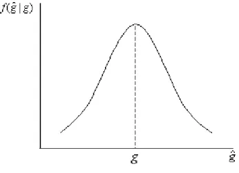
A chosen expenditure level g and a noise will determine the observed
policymaker’s type f(:j:) is equal to the density function of the noise that would yieldbgwhen the policy level is the one chosen by this type in equilibrium.
That is,
f(bgt=bgj t= i) =
lnbg lnGi
(10)
where is the density of the standard normal distribution. Figure 1 illustrates
the density function of the observed policy, for a given policy chosen.
Figure 1: Observed policy density function
Then, we can write the conditions for reelection in equation (9) as:
lnbg lnGf
> lnbg lnG
c
: (11)
In the case of a separating equilibrium, withGf > Gc, the policy has a cuto¤
levelg, such that, whenever the observed policy level is larger thang (bg > g), the median voter reelects the incumbent. This policy cuto¤ level is implicitly
de…ned by:
lng lnGf
= lng lnG
c
which, due to the symmetry of the normal distribution, is:
g= exp lnG
f+ ln
Gc
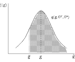
Figure 2: Policy Cuto¤ Level
Figure 2 depicts the density functions of the observed policy when the policy
level is the one chosen by each type of incumbent in equilibrium, f and c. The
…gure also shows the cuto¤ level of the observed policyg. Note that condition
(11) is satis…ed forbg > g.
For a chosen policyg, the reelection probability (q(:)) is the probability that the observed policy (bg) exceeds the cuto¤ point (g),9 that is:
q g; Gf; Gc Pr [bg > g] = Pr [ge > g] = = Pr [ >lng lng];
which can be written as:
q g; Gf; Gc = 1 lng lng ,
where (:)is the normal cumulative distribution function. The reelection prob-ability is increasing ing;and it is greater than 1
2 if, and only if, g > g. Figure
9More precisely, the probability of reelection is equal to the probability of the observed
Figure 3: Probability of reelection
3 illustrates the probability of reelection for a chosen policy levelgand for the
two types of incumbent equilibrium strategies,Gf andGc, which determineg.
Suppose, alternatively, that there is a separating equilibrium withGc> Gf
(we will see later that this equilibrium is not possible). Then, since voting is
prospective, the median voter will still prefer the policymaker further away from
the lobby, although she will choose a lower policy level before election. As a
consequence, the inference problem is reversed, and the probability of reelection
as a function of policy level and equilibrium strategy will become:
q g; Gf; Gc = lng lng ,
Now q is decreasing in g, since a lower g increases the probability that the
incumbent is of the distant type.
Finally, in the case of a pooling equilibrium, we have always =p. Thus, the probability of reelection is 12 and will not be a¤ected by any deviation from
equilibrium strategy.
function on the various types of equilibrium as follows:
q g; Gf; Gc =
8 > > < > > :
1 lng lng
;ifGf > Gc
lng lng
; ifGf < Gc
1
2 ifG
f =Gc
, (12)
whereg= exphlnGf+lnGc
2
i
.
4.2.3 The Incumbent’s Strategy
LetF W( i) be the after election utility of the type i government, when
re-elected:
F W( i) W Gi+1; I
i
+1; i
where Gi
+1 is the expenditure and I+1i is the decision of setting or not a deal
with the lobby, optimally chosen after elections by the reelected incumbent of
type i. Note that:
F W( i) U(g ); (13)
since it is always possible to the policymaker not to make a deal with the lobby
and to choose policy levelg . Moreover, the policymaker will be strictly better
o¤ being reelected if her proximity to the lobby enables her to get rents from
being in power.
When the incumbent is not reelected her utility will be the benevolent one,
since we assume that there is no additional source of personal income or loss of
reputation when the policymaker is not in o¢ce. LetF U be the expected after
election utility of the incumbent, when she is not reelected:
F U =pU Gf+1 + (1 p)U Gc+1 :
Since the policymaker will have no rents when she is not reelected, the best
outcome for her is to have the new incumbent setting policy level g . When
we make,10 her policy choice yields the defeated policymaker a lower utility
compared to that resulting fromg , thus:
F U < U(g ): (14)
Combining equations (13) and (14), we have that:
F U < F W( i): (15)
This last inequality implies that the policymaker always strictly prefers to
be reelected. Remember that rents are generated by the potential deal between
the policymaker in power and the lobby. Since those rents will depend on the
policy implemented, they are endogenous. The di¤erenceF W( i) F U has the
same role as the exogenous “ego rents” extensively used in the political economy
literature.
In equilibrium, the two decisions - the policy level and to set a deal or not
with the lobby - will be chosen to solve:
max
g;I V g; i; I; G f
; Gc (16)
s.t. g >0,
where:
V g; i; I; Gf; Gc =W(g; i; I)+ (17)
+ q g; Gf; Gc F W( i) + 1 q g; Gf; Gc F U ;
and where is the incumbent’s discount rate and the function q is given by
equation (12).
1 0As we argue below, after elections the incentives are more favorable to a deal. If we
assume functional forms and parameter values such that no deals are set after elections, the model will generate only an uninteresting pooling equilibrium with the utilitarian policyg
Equation (17) can be rewritten as:
V g; i; I; Gf; Gc = (18)
W(g; i; I) + q g; Gf; Gc [F W( i) F U] + F U;
which makes clear that a higher reelection probability increases the utility of
the incumbent whenever it is advantageous for one of the types to set a deal
with the lobby after election.
Whenever reelection increases utility, the incumbent policymaker will choose
a policy which will depart from the static optimal level - the one that maximizes
W(g; i; I). As we will show below, the only type of equilibrium consistent with
this possibility has Gf > Gc. This makes q increasing in g (equation (12)),
and the optimal level ofg higher than the static one for both types.11 As the
after election policy choices coincide with the static optimal choices, there will
be policy cycles around elections, with policy favoring more the people before
elections than after elections.
4.3
Equilibrium
An equilibrium requires a …xed point in the solution of the incumbent problem
(16). That is:
Gc = arg max
g;I
V g; c; I; Gf; Gc (19)
s.t. g >0,
1 1Formally, let Gj
+1 be the after election optimal expenditure for type j. Then @W(Gj+1; i;I)
@g = 0. Hence,
@V Gj+1; i; I; Gf; Gc
@g =
@W(Gj+1; i; I)
@g +
@q Gj+1; Gf; Gc
@g [F W( i) F U]
=
@q Gj+1; Gf; Gc
and:
Gf = arg max
g;I
V g; f; I; Gf; Gc (20)
s.t. g >0.
We can sum up the conditions for an equilibrium, when it exists, as follows.
A perfect Bayesian equilibrium in pure strategies, when it exists, should satisfy
the following conditions:
1. after election an incumbent of type j will choose to make a deal with
the lobby whenever its type j < , where is de…ned implicitly by
equation (6), and sets policy levelg#if she has a deal with the lobby and
g otherwise;
2. before election an incumbent chooses to set a deal or not with the lobby
and the policy level to maximize her expected intertemporal utility
func-tion, that is, to solve problem (16), where the probability of reelection
functionq(g; Gc; Gf)is given by expression (12);
3. the policy level for each type is a …xed point, that solves problems (19)
and (20), respectively.
We assume that the parameter values are such that the type closer to the
lobby bene…ts substantially from a deal with the lobby after election. This
will produce an equilibrium with the following features. First,Gf > Gc. An
equilibrium with Gf < Gc is not possible, since in this case the probability
function will be decreasing ingand the type c will choose a lower policy level
than f.
Second, there will be policy cycles around elections, that is, policy favors
more the people before elections than after. More precisely, whenever is
elections, there will be electoral incentives that stimulate a policy more favorable
to the poor before election than after for each policymaker type.
The third feature is that a deal between the policymaker and the lobby is
more likely to happen after election than before. More speci…cally, whenever
an incumbent of a certain type makes a deal with the lobby before election,
she will also do it after election, but the converse is not true. A deal with the
lobby is pro…table for the incumbent only if the policy favors substantially this
group. However, elections induce the policymaker to set a policy more favorable
to the people, reducing the gain of an agreement with the lobby. Therefore an
agreement with the lobby is less likely before elections.
There is no guarantee that a pure strategy equilibrium exists. The model
may not have an equilibrium if the type closer to the lobby bene…ts only
mar-ginally from a deal with the lobby after election. The argument is outlined in
Appendix C. However, a parameter con…guration which leads to no equilibrium
is not plausible in the context of the present model. The model relies on the
pos-sibility of deals between the policymaker and the lobby, and on non-observable
comparative advantages of certain types to bene…t from those deals. Thus, it is
reasonable to assume that those deals bene…t substantially (not marginally) the
type most attracted to them, c, under the most favorable conditions to them,
that is, after elections.
For the same reason, a con…guration of parameters for which the type closer
to the lobby would not make a deal after elections is not plausible either. This
would yield an uninteresting pooling equilibrium where both types would never
make a deal with the lobby and would choose the same policyg before and
5
Applications
5.1
Government expenditure cycles
5.1.1 Expenditure composition cycles
There is evidence of electoral cycles on the composition of the …scal budget in
several countries (on US, see Peltzman 1992; on Canada, see Kneebone and
McKenzie 2001; on Mexico, see Gonzalez 2004; on Colombia, see Drazen and
Eslava 2005). We now show how the framework developed above can be applied
to generate such electoral expenditures composition cycles.
In the simple formulation we choose, taxes are …xed and there are two types
of public goods, speci…c to each of the two groups. The government budget
constraint is represented by:
= (1 n)gl+ngp;
where , gl and gp are taxes, expenditures for the lobby and for the people,
respectively (all per capita). It can be rearranged as:12
gl=
ngp
1 n :
The utility function of a citizen of groupi, ui, is represented by:
ui(ci; gi) =ci+ loggi, fori=p; l, and >1;
whereci is her private consumption, andgi is the amount of the public
expen-diture available to her group. Given thatci =yi , indirect utility functions
may be written as:
vl(g) = yl + log
ng
1 n , and (21) vp(g) = yp + logg; (22)
1 2Note that, in this case, it is economically reasonable to impose an upper bound forg
p
(0< gp n) to prevent a negative value forgl. However, this new restriction is never binding
where we useg=gp for simplicity.
Substituting equations (21) and (22) into the utilitarian welfare function of
a benevolent policymaker, represented by equation (1), we get:
U(g) =y +nlogg+ (1 n) log ng
1 n ; (23) where y = nyp+ (1 n)yl is the average per capita income. The benevolent
policymaker would optimally choose:
g = =gl; (24)
that is, all citizens would receive the same spending level.
The optimal spending level under a deal in a one-period setting, that is, the
spending level that satis…es equation (5), is given by:
g#=
1 + b: (25) Note that in this application we have an explicit solution for the spending level.
It is easy to check Proposition 1: g#< g andg# is decreasing in .
The cuto¤ probability de…ned by equation (6) now becomes implicitly
de…ned by:
(1 n+ b) log1 n+ b
(1 n) (1 + b) log (1 + b) =X(1 ): (26)
Following the setup above, we are able to show that there will be an electoral
cycle in the expenditures composition, with more spending for the people before
than after election. We provide a numerical example to illustrate the model’s
ability to generate electoral cycles.
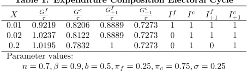
Numerical example Table 1 presents examples of the three possible
equilib-rium types. The examples di¤er in the value of the lossXdue to an unsuccessful
c = 0:75, n = 0:7, b = 0:5, = 0:25, p= 0:5, and = 0:9 . The …rst line
presents the results for a relatively small value forX,0:01, which makes a deal with the lobby always bene…cial to both types before and after elections. We
ob-serve that there is an expenditures cycle for both incumbent types, with higher
expenditures for the people before elections.
Table 1: Expenditure Composition Electoral Cycle
X Gf Gc G
f
+1 G
c
+1
If Ic I+1f I+1c
0.01 0.9219 0.8206 0.8889 0.7273 1 1 1 1 0.02 1.0237 0.8122 0.8889 0.7273 0 1 1 1 0.2 1.0195 0.7832 1 0.7273 0 1 0 1 Parameter values:
n= 0:7; = 0:9; b= 0:5; f = 0:25; c= 0:75; = 0:25
When we increaseX to0:02, we generate additionally a lobby activity elec-toral cycle. Before the election, a deal with the lobby becomes not advantageous
to the type less connected with the lobby, despite being bene…cial after election.
In order to increase her reelection probability, the policymaker of this type
prefers to increase her expenditure to the people to a level above the optimal
one, distorting expenditure in a direction opposed to the lobby interests.
Increasing the damage of an unsuccessful deal further, toX= 0:2, will make even an after election agreement with the lobby not bene…cial to the distant type
policymaker. However, the close type, having a higher probability of success in
the deal with the lobby, is still able to pro…t from the agreement, before and
after elections. We still have an expenditure cycle, with the close type choosing
to set a deal with the lobby before and after election, and the distant type not
setting the deal at any time.
Finally, an increase ofX to the point that prevents any deal with the lobby
(not presented in the table) will result in an not very interesting type of
elections.13
5.1.2 Aggregate expenditure cycles
Electoral cycles in aggregate expenditures can be generated by a simple change
in the model described above. Suppose that the people are not taxed and receive
the only public good. Indirect utility functions become:
vl(g) = yl , and (27)
vp(g) = yp+ logg: (28)
We still assume a balance budget: g= :
An utilitarian policymaker without lobby in‡uence and electoral incentives
will choose:
g = n 1 n:
If the policymaker chooses to spendg < g , she can increase the lobby group
utility byg g and get a share B(g g ). Hence, if she has a deal with the lobby, she would choose:
g#= n 1 n+ b =
g
1 + gnb; (29)
whereb [ (1 n)]B.
With information asymmetry about the two di¤erent policymaker types,
c and f, as before, the model generates electoral cycles in aggregate
expen-ditures. This result is in line with the empirical evidence, as in Brender and
Drazen (2004), Shi and Svensson (2002a,b), and Persson and Tabellini (2002).14
1 3As common in political business cycle models, a reverse cycle may happen, although with
lower probability, when a incumbent closer to the lobby looses the election for an opponent of the other type.
1 4Note that the balanced budget assumption also generates a counterfactual electoral tax
Moreover, the mechanism in our paper, which is based on policymakers
receiv-ing personal bene…ts from interest groups, is consistent with the evidence
pro-vided by Shi and Svensson (2002b). They show that political budget cycles are
stronger in countries with higher corruption and rent seeking indicators.
5.2
Exchange rate cycles
There is empirical evidence of exchange rate electoral cycles for Latin American
countries (cross-country evidence for Latin America is provided by Frieden,
Ghezzi and Stein, 2001, and Ghezzi, Stein and Streb, 2004, for Brazil, see
Bonomo and Terra, 2001, Grier and Hernández-Trillo, 2004, for Mexico, and
Pascó-Fonte and Ghezzi, 2001, for Peru). Bonomo and Terra (2005) presents
a model that generates real exchange rate electoral cycles, in a setting with
informational asymmetry over the policymaker’s preferences. Here we derive the
same result in a simpler model based of the special interests politics proposed
in this paper.
Consider a endowment economy with two sectors: a tradable a nontradable
sector. The nontradable sector has the majority of the population, while the
tradable sector has the lobby power. All consumers are assumed to have the
same CES utility function:
u(Ni; Ti) = N
r
1+r
i +T
r
1+r
i
1+r r
; (30)
whereNi andTi are the amount consumed of nontradable and tradable goods,
respectively, andr >1. Now letebe the tradable good relative price, which is the real exchange rate. De…neg 1e As expected, the indirect utility function
is decreasing in the real exchange rate for a citizen in the nontradable sector,
and increasing for the tradable sector:
vN(e) = 1 +g r
1
rEN, and (31)
vT(e) = (1 +gr)
1
whereEN andET are the per capita endowment for the nontradable and
trad-able sectors, respectively.
A benevolent (utilitarian) policymaker would choose to set the exchange rate
at a level:15
g = nE
N
(1 n)ET
1
r 1
: (33)
The policymaker may choose to set a more depreciated exchange rate,g < g
(which meanse > e g1) in order to favor the tradable sector and get a share
of its gain. Proceeding as before, we …nd that when there is an agreement with
the tradable sector the chosen exchange rate is given by:
g# = nE
N
(1 n)ET + bET
1
r 1
(34)
= g 1 n
1 n+ b
1
r 1
(35)
By assuming that there are two types of policymakers, c and f,
informa-tion asymmetry engenders a mechanism by which exchange rate electoral cycles
are generated. The policymaker will choose a more appreciated exchange rate
before than after election.
6
Conclusion
Special interest politics is often associated with microeconomic policy, and its
macroeconomic impact is thought to be negligible. Here we are concerned with
opposite interests which divide the entire society in two groups: one with the
lobby power, and the other with the majority of votes. Government policy may
a¤ect the distribution of resources in the society between those two groups.
1 5We implicitly assume that the government manipulates its expenditure level in
In this paper we propose a link between special interest politics and political
business cycles. We build a framework where the lobby power of a special
interest group interacts with the voting power of the majority of the population,
leading to political business cycles. The model generates an additional cycle,
which is a “contracting” cycle around elections. Since reelection concerns induce
the policymaker to favor less the lobby group, the mutual net gains from a deal
between the incumbent and the lobby are reduced before elections. Therefore, it
is less likely that the policymaker will make a deal with the lobby group before
elections than after elections.
We showed that those same ideas could be applied to generate cycles around
election in other economic variables, such as government expenditures level, and
the real exchange rate.
The mechanism we propose in this paper does not exclude the operation of
traditional political business cycle channels, as proposed by the opportunistic
and partisan literature. The relative importance of our proposed channel in
explaining the electoral cycle in di¤erent variables should be investigated in
future research.
Appendix A: When an unsuccessful deal is revealed to the public
In this appendix we drop the assumption that the incumbent incurs in an
exogenous utility loss when her deal with the lobby is not successful. We assume,
instead, that an unsuccessful deal is revealed to the public. In this case, the
policymaker’s loss from an unsuccessful deal will be due to the e¤ect of this
revelation on her reelection probability.
The policymaker preferences are now represented by:
f
which implies the following indirect utility function:
W0(g; I; ) =U(g) +I b[v
l(g) vl(g )], (36)
whereb (1 n) ( 1)B.
In this model, both types of incumbent will choose to make a deal with
the lobby after election, as there is no penalty from an unsuccessful deal. The
optimal after election policy chosen is also implicitly de…ned by equation (5).
Before election, the incumbent will take into account the e¤ect of the chosen
policy on her reelection probability. Here we will restrict our analysis to the
case in which there exists an equilibrium where, before election, the incumbent
closer to the lobby chooses to make a deal, while the other type does not.
Now the voter observes, not only the policy (with noise), but also whether
there was an unsuccessful deal. Let j be the voter’s updated belief that the
incumbent is of type f, after observingbgand whether an unsuccessful deal
oc-curred or not (Ix=jwithj= 1when the deal is unsuccessful and0otherwise).
Formally:
j= Pr ( t= fjbgt=bg; Ix=j)
If an unsuccessful deal occurs, the voter will infer that the policymaker type
is f. Therefore 1= 0, and the incumbent will not be reelected.
The updated belief when the voter receives no signal of an unsuccessful deal
is:
0=
p h(bgt=bg; Ix= 0j t= f)
p h(bgt=g; Ib x= 0j t= f) + (1 p) h(bgt=bg; Ix= 0j t= c)
;
(37)
whereh(bgt=g; Ib x= 0j t= i)is the joint density of observing a policy signal
b
gand receiving no information about an unsuccessful deal, given the incumbent
It is clear that:
h(bgt=bg; Ix= 0j t= c) = c f(bgt=bgj t= c); and (38)
h(bgt=bg; Ix= 0j t= f) = f(bgt=bgj t= f);
since the success of the deal is assumed to be independent of the policy chosen
by the incumbent when the incumbent makes a deal with the lobby.
When the voters receive no information about an unsuccessful deal, the
incumbent will be reelected if 0 > p, which, after substituting equation (38)
into (37), can be seen to be equivalent to:
f(bgt=bgj t= f)> c f(bgt=bgj t= c):
Given the assumed lognormal distribution for the noise, the cuto¤ for the
observed policy signalegwill be given by:
lneg=lnG
f+ lnGc
2 +
ln c
lnGf lnGc
The reelection probability for an incumbent which chooses a policy g and
whether to set a dealIcan easily be shown to be given by:
q0 g; I; Gf
; Gc = [1 I(1 i)] 1
lneg lng
. (39)
Note that the reelection probability decreases when the incumbent chooses
to make a deal with the lobby.
The intertemporal utility function of the incumbent becomes:
V0 g; I; i; Gf; Gc = (40)
W0(g; I;
i) + q0 g; I; Gf; Gc [F W( i) F U] + F U:
Observe that, whenI= 0; V0(:)becomes the same function as in the original
it depends on Gc. The closer type faces a di¤erent objective function, as the
reelection probability is a di¤erent function ofg.
Appendix B: A multiperiod framework
Here we sketch the problem in a multiperiod framework. The main
modi-…cation is in de…ning a value function for the incumbent problem and solving
it by dynamic programming. Instead of breaking the value function into one
period pieces, as usual, here it is appropriate to break it into two-period pieces.
Let Y( i) be the value function for the type i. Then we have a pair of
Bellman equations:
Y( i) = max
g;I W(g; i; I) +
q g; Gf; Gc F W( i) +
1 q g; Gf; Gc 1F U +
+ 2q g; Gf; Gc [pY ( f) + (1 p)Y ( c)] fori=f; c
where we assumed that once the incumbent looses the election, she will be a
regular citizen forever.
As before, in equilibriumGf; Gc solves the problem fori=c; f. Then, we
have
Y( i) =W(Gi; i; Ii) +
F U
1 +
+ q Gi; Gf; Gc F W( i) + (pY ( f) + (1 p)Y( c))
F U
1
for i=f; c
The term between square brackets represents the gain from being reelected,
and we will show that it is strictly positive and greater than the rents from
being reelected once,F W( i) F U >0. It can be rewritten as:
F W( i) F U+ (pY ( f) + (1 p)Y( c))
F U
In order to evaluate the term between square brackets, note that:
Y( i) U(g ) +
F U
1 fori=f; c,
since in the …rst period the incumbent is in charge and g is in her policy
choice set. As for the continuing utility, if she is not reelected, she will get
F U thereafter. If she is reelected, her continuing utility is greater thanF U, as
shown in equation (15).
Furthermore, using equation (14), we also have that:
U(g ) + F U 1 >
F U
1 :
Combining the two inequalities above, we have that:
Y( i)>
F U
1 fori=f; c.
which implies:
(pY ( f) + (1 p)Y ( c))
F U
1 >0:
Hence, this result renders the incumbent a gain greater thanF W( i) F U
from being reelected. Thus, the incentives for getting reelected are even higher,
leading to more pronounced cycles, in this multiperiod setting.
Appendix C: Conditions under which there is no pure strategy
equilibrium
The model may not have an equilibrium if the type closer to the lobby
bene…ts only marginally from a deal with the lobby after election. The argument
is outlined below.
Let the parameters be such that the policymaker of type copt for a contract
after election but for no contract before. As we will argue, this happens when
0 < c < ", for a su¢ciently small positive ", where is the probability
chooses to make a deal with the lobby after election and distorts policy. Thus,
F W( j) > F U for both incumbent types, that is, they strictly prefer to be
reelected. For this reason, both incumbent types have an incentive to distort
policy to increase their reelection probability. Assume that, in equilibrium,
Gf > Gc, so that the reelection probability is increasing in g (by equation
(12)). The policymaker of type c will face a con‡ict of incentives between a
policy which leads to a higher probability of reelection - a higherg- and a policy
which will lead to higher personal bene…ts - a lowerg. However, for a su¢ciently
low " the deal with the lobby after elections is only marginally advantageous
to her, so that the additional electoral incentive makes a deal with the lobby
before election not advantageous. It is clear that the incumbent of type f will
have even less incentives to set a deal with the lobby before elections, since
she faces a higher probability of a bad outcome. Hence, neither incumbent
types set a deal with the lobby before election. Their di¤erent incentives in
the pre-election policy choice comes from their di¤erent electoral incentives.
SinceF W( c) F U > F W( f) F U, the policymaker of type c will have a
higher reelection gain, therefore she will make a higher e¤ort to be reelected by
choosing a higherg. That is,Gf < Gc, which contradicts our initial assumption
thatGf > Gc.
An equilibrium withGf < Gc is not possible either, since in this case the
probability function will be decreasing ing and the type c will choose a lower
policy level than f. Then, the only remaining possibility is a pooling
equi-librium, with both types choosing policy levelg . However, this cannot be an
optimal choice for type c, since in this case the incentives the policymaker faces
before election are the same she does after election, when she chooses to have a
deal with the lobby.
CIREQ
Graduate School of Economics/Fundacao Getulio Vargas
References
[1] Alesina, A. (1987), “Macroeconomic Policy in a Two-Party System as a
Repeated Game,”Quarterly Journal of Economics 102: 651-78.
[2] Bonomo, M. and C. Terra (2005). “Elections and Exchange Rate Policy
Cycles,”Economics and Politics 17(2): 151-176.
[3] Bonomo, M. and C. Terra (2001), “The Dilemma of In‡ation vs. Balance of
Payments: Crawling Pegs in Brazil, 1964-98,” in: J. Frieden and E. Stein,
eds.,The Currency Game: Exchange Rate Politics in Latin America(IDB,
Washington).
[4] Brender, A. and A. Drazen (2004), “Political Budget Cycles in New Versus
Established Democracies,” NBER Working Paper 10539.
[5] Cukierman, A. and A.Meltzer (1986), “A Positive Theory of Discretionary
Policy, the Costs of Democratic Government, and the Bene…ts of a
Consti-tution,” Economic Inquiry 24: 367-88.
[6] Dixit, A. (2004),Lawlessness and Economics, Princeton University Press.
[7] Downs, Anthony (1957),An Economic Theory of Democracy, Addison
Wes-ley.
[8] Drazen, A. and M. Eslava (2005a), “Electoral Manipulation via
Expendi-ture Composition: Theory and Evidence,” NBER Working Paper 11085.
[9] Drazen, A. and M. Eslava (2005b), “Political Budget Cycles When
[10] Frieden, J. and E. Stein (2001),The Currency Game: Exchange Rate
Pol-itics in Latin America, IDB, Washington.
[11] Frieden, J., P. Ghezzi and E. Stein (2001), “Politics and Exchange Rates:
A Cross Country Study,” in: J. Frieden and E. Stein, eds., The Currency
Game: Exchange Rate Politics in Latin America (IDB, Washington).
[12] Ghezzi, P., E. Stein and J. Streb (2004), “Real Exchange Rate Cycles
around Elections,”Economics and Politics, forthcoming.
[13] Gonzalez, Maria de los A. (2004), “Do Changes in Democracy A¤ect the
Political Budget Cycle?,”Review of Development Economics,forthcoming.
[14] Grier, Kevin B. and Fausto Hernández-Trillo (2004), “The Real Exchange
Rate Process and Its Real E¤ects,” Journal of Applied Economics VII(1):
1-25
[15] Grossman, Gene and Elhanan Helpman (1994), “Protection for Sale,”
American Economic Review 84: 833-50.
[16] Grossman, Gene and Elhanan Helpman (1996), “Electoral Competition and
Special Interest Politics,”Review of Economic Studies 63: 265-286.
[17] Grossman, Gene and Elhanan Helpman (2001), Special Interest Politics,
MIT Press.
[18] Hibbs, D. (1977), “Political Parties and Macroeconomic Policy,”American
Political Science Review 71: 146-87.
[19] Holmstrom, Bengt (1999), “Managerial Incentive Problems: A Dynamic
Perspective,”Review of Economic Studies 66: 169-182.
[20] Kneebone, R. and K. McKenzie (2001), “Electoral and Partisan Cycles in
Fiscal Policy: an Examination of Canadian Provinces,” International Tax
[21] Lindbeck, A. (1976), “Stabilization Policies in Open Economies with
En-dogenous Politicians,”American Economic Review Papers and Proceedings,
1-19.
[22] Nordhaus, W. (1975), “The Political Business Cycle,”Review of Economic
Studies 42: 169-90.
[23] Pascó-Fonte, A. and P. Ghezzi (2001), “Exchange Rates and Interest
Groups in Peru, 1950-1996,” in: J. Frieden and E. Stein, eds.,The Currency
Game: Exchange Rate Politics in Latin America (IDB, Washington).
[24] Peltzman, S. (1992), “Voters as Fiscal Conservatives,” Quarterly Journal
of Economics 107: 327-361.
[25] Persson, T. and G.Tabellini (2000),Political Economics: Explaining
Eco-nomic Policy (The MIT Press).
[26] Persson, T. and G.Tabellini (2002), “Do Electoral Cycles Di¤er Across
Political Systems?,” working paper.
[27] Rogo¤, K. (1990), “Equilibrium Political Budget Cycles,”American
Eco-nomic Review 80: 21-36.
[28] Rogo¤, K. and A. Silbert (1988), “Elections and Macroeconomic Policy
Cycles,”Review of Economic Studies 55: 1-16.
[29] Shi, E. and J. Svensson (2002a), “Conditional Political Business Cycles,”
CEPR Discussion Paper #3352.
[30] Shi, E. and J. Svensson (2002b), “Political Business Cycles in Developed
and Developing Countries,” mimeo.
[31] Sims, C. (2003), “Implications of Rational Inattention,”Journal of
´
Ultimos Ensaios Econˆomicos da EPGE
[576] Andrew W. Horowitz e Renato Galv˜ao Flˆores Junior. Beyond indifferent players:
On the existence of Prisoners Dilemmas in games with amicable and adversarial preferences. Ensaios Econˆomicos da EPGE 576, EPGE–FGV, Dez 2004.
[577] Rubens Penha Cysne. Is There a Price Puzzle in Brazil? An Application of
Bias–Corrected Bootstrap. Ensaios Econˆomicos da EPGE 577, EPGE–FGV,
Dez 2004.
[578] Fernando de Holanda Barbosa, Alexandre Barros da Cunha, e Elvia Mureb Sal-lum. Competitive Equilibrium Hyperinflation under Rational Expectations. En-saios Econˆomicos da EPGE 578, EPGE–FGV, Jan 2005.
[579] Rubens Penha Cysne. Public Debt Indexation and Denomination, The Case
of Brazil: A Comment. Ensaios Econˆomicos da EPGE 579, EPGE–FGV, Mar
2005.
[580] Gina E. Acosta Rojas, Germ´an Calfat, e Renato Galv˜ao Flˆores Junior. Trade and
Infrastructure: evidences from the Andean Community. Ensaios Econˆomicos da
EPGE 580, EPGE–FGV, Mar 2005.
[581] Edmundo Maia de Oliveira Ribeiro e Fernando de Holanda Barbosa. A Demanda
de Reservas Banc´arias no Brasil. Ensaios Econˆomicos da EPGE 581, EPGE–
FGV, Mar 2005.
[582] Fernando de Holanda Barbosa. A Paridade do Poder de Compra: Existe um
Quebra–Cabec¸a?. Ensaios Econˆomicos da EPGE 582, EPGE–FGV, Mar 2005.
[583] Fabio Araujo, Jo˜ao Victor Issler, e Marcelo Fernandes. Estimating the Stochastic
Discount Factor without a Utility Function. Ensaios Econˆomicos da EPGE 583,
EPGE–FGV, Mar 2005.
[584] Rubens Penha Cysne. What Happens After the Central Bank of Brazil Increases
the Target Interbank Rate by 1%?. Ensaios Econˆomicos da EPGE 584, EPGE–
FGV, Mar 2005.
[585] GUSTAVO GONZAGA, Na´ercio Menezes Filho, e Maria Cristina Trindade Terra. Trade Liberalization and the Evolution of Skill Earnings Differentials
in Brazil. Ensaios Econˆomicos da EPGE 585, EPGE–FGV, Abr 2005.
[586] Rubens Penha Cysne. Equity–Premium Puzzle: Evidence From Brazilian Data. Ensaios Econˆomicos da EPGE 586, EPGE–FGV, Abr 2005.
[587] Luiz Renato Regis de Oliveira Lima e Andrei Simonassi. Dinˆamica N˜ao–Linear
e Sustentabilidade da D´ıvida P´ublica Brasileira. Ensaios Econˆomicos da EPGE
[588] Maria Cristina Trindade Terra e Ana Lucia Vahia de Abreu. Purchasing Power
Parity: The Choice of Price Index. Ensaios Econˆomicos da EPGE 588, EPGE–
FGV, Abr 2005.
[589] Osmani Teixeira de Carvalho Guill´en, Jo˜ao Victor Issler, e George Athanasopou-los. Forecasting Accuracy and Estimation Uncertainty using VAR Models with
Short– and Long–Term Economic Restrictions: A Monte–Carlo Study. Ensaios
Econˆomicos da EPGE 589, EPGE–FGV, Abr 2005.
[590] Pedro Cavalcanti Gomes Ferreira e Samuel de Abreu Pessˆoa. The Effects of
Longevity and Distortions on Education and Retirement. Ensaios Econˆomicos
da EPGE 590, EPGE–FGV, Jun 2005.
[591] Fernando de Holanda Barbosa. The Contagion Effect of Public Debt on
Mo-netary Policy: The Brazilian Experience. Ensaios Econˆomicos da EPGE 591,
EPGE–FGV, Jun 2005.
[592] Rubens Penha Cysne. An Overview of Some Historical Brazilian
Macroeco-nomic Series and Some Open Questions. Ensaios Econˆomicos da EPGE 592,
EPGE–FGV, Jun 2005.
[593] Luiz Renato Regis de Oliveira Lima e Raquel Menezes Bezerra Sampaio. The
Asymmetric Behavior of the U.S. Public Debt.. Ensaios Econˆomicos da EPGE
593, EPGE–FGV, Jul 2005.
[594] Pedro Cavalcanti Gomes Ferreira, Roberto de G´oes Ellery Junior, e Victor Go-mes. Produtividade Agregada Brasileira (1970–2000): decl´ınio robusto e fraca
recuperac¸˜ao. Ensaios Econˆomicos da EPGE 594, EPGE–FGV, Jul 2005.
[595] Carlos Eugˆenio Ellery Lustosa da Costa e Lucas J´over Maestri. The
Interac-tion Between Unemployment Insurance and Human Capital Policies. Ensaios
Econˆomicos da EPGE 595, EPGE–FGV, Jul 2005.
[596] Carlos Eugˆenio Ellery Lustosa da Costa. Yet Another Reason to Tax Goods. Ensaios Econˆomicos da EPGE 596, EPGE–FGV, Jul 2005.
[597] Marco Antonio Cesar Bonomo e Maria Cristina Trindade Terra. Special Interests
and Political Business Cycles. Ensaios Econˆomicos da EPGE 597, EPGE–FGV,
Ago 2005.
[598] Renato Galv˜ao Flˆores Junior. Investimento Direto Estrangeiro no Mercosul:
Uma Vis˜ao Geral. Ensaios Econˆomicos da EPGE 598, EPGE–FGV, Ago 2005.
[599] Aloisio Pessoa de Ara´ujo e Bruno Funchal. Past and Future of the Bankruptcy
Law in Brazil and Latin America. Ensaios Econˆomicos da EPGE 599, EPGE–
FGV, Ago 2005.
[600] Marco Antonio Cesar Bonomo e Carlos Carvalho. Imperfectly Credible
Disin-flation under Endogenous Time–Dependent Pricing. Ensaios Econˆomicos da