Asymmetry parameter for nonmesonic hypernuclear decay
Cesar Barbero
Departamento de F´ısica, Facultad de Ciencias Exactas, Universidad Nacional de La Plata, C.C. 67, 1900 La Plata, Argentina
Alfredo P. Gale˜ao
Instituto de F´ısica Te´orica, Universidade Estadual Paulista, Rua Pamplona 145, 01405-900 S˜ao Paulo, SP, Brazil
Francisco Krmpoti´c
Instituto de F´ısica, Universidade de S˜ao Paulo, C. P. 66318, 05315-970 S˜ao Paulo, SP, Brazil, Instituto de F´ısica La Plata, CONICET, 1900 La Plata, Argentina, and
Facultad de Ciencias Astron´omicas y Geof´ısicas, Universidad Nacional de La Plata, 1900 La Plata, Argentina
(Received 11 February 2005; revised manuscript received 30 June 2005; published 28 September 2005)
We give general expressions for the vector asymmetry in the angular distribution of protons in the nonmesonic weak decay of polarized hypernuclei. From these we derive an explicit expression for the calculation of the asymmetry parameter, a, which is applicable to the specific cases of 5He and
12
C described within the
extreme shell model. In contrast to the approximate formula widely used in the literature, it includes the effects of three-body kinematics in the final states of the decay and correctly treats the contribution of transitions originating from single-proton states beyond thes-shell. This expression is then used for the corresponding numerical computation ofawithin several one-meson-exchange models. Besides the strictly local approximation usually
adopted for the transition potential, we also consider the addition of the first-order nonlocality terms. We find values fora ranging from−0.62 to−0.24, in qualitative agreement with other theoretical estimates but in
contradiction with some recent experimental determinations.
DOI:10.1103/PhysRevC.72.035210 PACS number(s): 21.80.+a, 13.75.Ev, 21.60.−n
I. INTRODUCTION
While thehyperon, in free space, decays 99.7% of the time through the mesonic mode,→π N, inside nuclei this is Pauli-blocked, and, already forA >∼5, the weak decay is gradually dominated by the nonmesonic channel,N →N N, where the large momentum transfers involved (≈400 MeV/c) put the two emitted nucleons above the Fermi surface. This decay mode is interesting since it offers a unique opportunity to probe the strangeness-changing weak interaction between hadrons. For a recent review of hypernuclear decay, see Ref. [1].
For a long time, the experimental data for this process was restricted to the full nonmesonic decay rate, Ŵnm, and, in some cases, also the partial ones,Ŵn=Ŵ(n→nn) and Ŵp=Ŵ(p→np). More recently, the first results, obtained at KEK [2–4], for another important observable of nonmesonic decay, namely, the intrinsic asymmetry parameter,a, have become available. This is experimentally more demanding, as it requires measuring the asymmetry in the angular distribution of protons emitted in the decay of polarized hypernuclei. On the theoretical side, however, a carries important new information, since it is determined by the interference terms between the parity-conserving (PC) and the parity-violating (PV) proton-induced transitions to final states with different isospins. In opposition to that, the decay rates depend only on the square moduli of the separate components of the transition potential, being dominated by the PC ones. One expects, therefore, that the asymmetry parameter, besides being more sensitive to the PV amplitudes, will have more discriminating power to constrain the proposed mechanisms for nonmesonic hypernuclear decay.
Most of the theoretical work on this decay mode constructs the transition potential by means of one-meson-exchange (OME) models, the most complete ones including up to the whole ground pseudoscalar and vector meson octets (π, η, K, ρ, ω, K∗) [5–7]. Recently we extended such models to take into account the kinematical corrections due to the difference between the lambda and nucleon masses and the first-order nonlocality terms [8]. There are also OME models that consider additional effects, such as correlated-two-pion exchange [9] and direct-quark interaction [10]. In all these cases, to which we will refer to below as strict OME models, the weak coupling constants for the pion are empirically deter-mined from the free mesonic decay, and those of the remaining mesons by means of unitary-symmetry arguments [5,6].
All such models reproduce quite easily the total non-mesonic decay rate, Ŵnm=Ŵn+Ŵp, but seem to strongly underestimate the experimental values for then/pbranching ratio, Ŵn/ Ŵp [1]. However, there are recent indications, based on the intranuclear cascade model, that this might be due to contamination of the data by secondary nucleons unleashed by final state interactions (FSI) while the primary ones are traversing the residual nucleus [11]. Another serious discrepancy between theory and experiment in nonmesonic decay concerns the asymmetry parameter. The measurements favor a negative value for 12
C and a positive value for
5
He. However, all existing calculations based on strict OME models [5,6,8–10] find values for a between −0.73 and
−0.19 [1,12]. Also, when results for 12
the particular hypernucleus considered. A recent attempt [12] to explain this discrepancy along similar lines to those used for then/pproblem has failed. As might be expected, the FSI do have an effect in attenuating the asymmetry, but show no tendency to reverse its sign. The only theoretical calculations that attain some agreement with the experimental data fora are a first application of effective field theory to nonmesonic decay [14] and a very recent extension of the direct-quark interaction model to include sigma-meson exchange [15]. However, in both cases, one or more coupling constants are specifically adjusted to reproduce the experimental value of afor5He.
Most calculations of the asymmetry parameter make use of an approximate formula [Eq. (43), below] which, however, is valid only for s-shell hypernuclei. Since an essential aspect in the asymmetry puzzle presented above concerns the comparison of its values for 5
He and 12C, it would be of great interest to have a simple expression that is applicable to both cases. This is the main objective of the present paper, in which a general formalism for the asymmetry parameter in nonmesonic decay is derived and subsequently particularized to these two hypernuclei. We start by presenting, in Sec. II, the main steps in the derivation of the general expression, Eq. (6), of the vector hypernuclear asymmetry in terms of decay strengths. This is equivalent to Eq. (27) of Ref. [13]. However, we deviate considerably from that reference from this point onwards. The main difference is that we do not make use of spectroscopic factors, but rather rely on spectroscopic amplitudes, which can then be computed in the nuclear structure model of choice. This has, in our view, two great advantages. Firstly, the spectroscopic amplitudes can be determined without any ambiguity as to their phases. This is particularly important for the asymmetry parameter, where, differently from the case of the decay rates, one is dealing with an interference phenomenon. Secondly, since, due to the large value of the momentum transferred in the fundamental process, nonmesonic decay is not significantly affected by details of nuclear structure, one can choose to work in the extreme shell model. Doing this, much of the summation over the final states of the residual nucleus can be explicitly performed, leading to very simple expressions for the asymmetry. [See, for instance, Eq. (42).] The scheme for computing the decay strengths by means of an integration over the available phase space is presented in Sec. III, and the summations needed for the asymmetry parameter are performed in Sec. IV. Finally, the numerical results obtained by applying this formalism to the calculation of a for, both 5He, and
12
C, in several strict OME models, are presented and discussed in Sec. V, where we also summarize our main conclusions. Details of the derivation of the final expression for a are given in Appendices A–C, and some identities that have been used for this purpose are listed in Appendix D.
II. VECTOR HYPERNUCLEAR ASYMMETRY Single- hypernuclei produced in a (π+, K+) reaction, under favorable kinematical conditions, are known to end up with considerable vector polarization along the direction
normal to the reaction plane, ˆn=(pπ+× pK+)/|pπ+×pK+|, of which they retain a significant amount,PV, even after they have cascaded down to their ground states by electromagnetic and strong processes [2,3,16]. Therefore, the initial mixed
state from which the hypernucleus will decay weakly can be described by the density matrix (Ref. [17], Eq. (9.29))
ρ(JI)= 1 2JI +1
1+ 3
JI+1
PVJI ·nˆ
, (1)
whereJI is the hypernuclear spin.
The angular distribution of protons emitted in the proton-induced nonmesonic decay, p→np, of the pure initial hypernuclear state |JIMI is given by Fermi’s golden rule as
dŴ(JIMI → pˆ2tp) dp2
=
dp1
dF
s1s2MF
|p1s1tnp2s2tpνFJFMF|V|JIMI|2.
(2) Here, p1s1 and p2s2 are the momenta and spin projections
of the emitted neutron and proton, respectively, and we have introduced the compact notation (¯h=c=1)
dF . . .=2π νFJF
p2
2dp2
(2π)3
p2
1dp1
(2π)3δ
×
p2
1
2M+ p2
2
2M+
|p1+p2|2
2MF −
δνFJF
. . . ,
(3) M being the nucleon mass; MF, that of of the residual nucleus, which is left in state|νFJFMF whereνF specifies the remaining quantum numbers besides those related to the nuclear spin; andνFJF, the liberated energy. (To avoid
confusion, we will be using Roman font (M,m) for masses and italic font (M, m) for azimuthal quantum numbers.) Also indicated in Eq. (2) are the isospin projections tn≡ −1/2 andtp≡ +1/2 of the neutron and proton, respectively. The transition amplitude includes both the direct and the exchange contributions, i.e.,
p1s1tnp2s2tpνFJFMF|V|JIMI
=(p1s1tnp2s2tpνFJFMF|V|JIMI
−(p2s2tpp1s1tnνFJFMF|V|JIMI, (4)
where the round bras stand for simple (nonantisymmetrized) product states for the emitted nucleons and the transition potential,V, is extracted from the Feynman amplitude for the direct process [8].
It is then possible to show [13,18], by taking the appropriate average of Eq. (2), that the angular distribution of protons from the decay of the polarized mixed state described by Eq. (1) has the form
dŴ[ρ(JI)→ pˆ2tp]
dp2 =
Ŵp
FIG. 1. Coordinate system for the calculation of decay strengths.
whereŴpis the full proton-induced decay rate, and thevector
hypernuclear asymmetry,AV, is given by
AV = 3 JI+1
MIMIσ(JIMI)
MIσ(JIMI)
. (6)
The new quantities introduced above are thedecay strengths, σ(JIMI)
=
dp1
dF
s1s2MF
|p1s1tnp2s2tpνFJFMF|V|JIMIp.h.f.|2,
(7) where the subscript p.h.f. indicates that one is dealing here with the transition amplitude in the proton helicity frame, in which the direction for angular momentum quantization is that of the proton momentum. Equivalently, one can choose, for the calculation of the decay strengths, a coordinate system having thez-axis pointing along the proton momentum, and proceed as usually. This is depicted in Fig. 1.
It is clear that, with the help of Eq. (5), one can extract the value of the product PVAV from the counting rates parallel and opposite to the polarization direction, by taking the ratio of their difference to their sum. Assuming that PV can also be independently measured, or calculated, this experimentally determines the vector hypernuclear asymmetry,AV.
III. DECAY STRENGTHS
To compute the decay strengths, it is convenient to rewrite the transition amplitudes in Eq. (7) in the total spin (S, MS)
and isospin (T , MT) basis. We start from the relation
|p1s1tnp2s2tp)− |p2s2tpp1s1tn)
=
SMST MT
(1/2s11/2s2|SMS)(1/2tn1/2tp|T MT)
×[|p PSMST MT)−(−)S+T|−p PSMST MT)], (8)
where we have also changed the representation to relative and total momenta, given, respectively, by
p= 12(p2−p1),
(9)
P = p1+p2.
Since we are takingtn≡ −1/2 andtp ≡ +1/2, we can write
(1/2tn1/2tp|T MT)= 1
√
2(δT1−δT0)δMT0, (10) and performing the transformation (8) in Eq. (4), we get
p1s1tnp2s2tpνFJFMF|V|JIMI
= −
SMS
(1/2s11/2s2|SMS)
×
T (−)T
p PSMST νFJFMF|V|JIMI, (11)
where we have defined
p PSMST νFJFMF|V|JIMI
=√1
2[(p PSMST νFJFMF|V|JIMI −(−) S+T
×(−p PSMST νFJFMF|V|JIMI], (12)
dropping, for simplicity, the MT =0 labels, as shall be done henceforth. Finally, introducing Eq. (11) into Eq. (7), and making use of the orthogonality of the Clebsch-Gordan coefficients in spin space, we are left with
σ(JIMI)=
dp1
dF
SMSMF
T (−)T
× p PSMST νFJFMF|V|JIMIp.h.f.
2
. (13)
For the integration in Eq. (13), there are six momentum variables involved, namely, the components of p1 and p2. These, however, are not all independent. The choice ofz-axis in Fig. 1 eliminates two angular variables. Also, the energy conservation condition in Eq. (3) gives one relation to be satisfied. This leaves 6−3=3 independent variables. A convenient choice is
Simple trigonometry, applied in Fig. 1, leads to the relations 4p2=p12+p22−2p1p2cosθp1,
P2=p12+p22+2p1p2cosθp1,
(15) cosθp =
p2−p1cosθp1
2p ,
cosθP =
p2+p1cosθp1
P ,
which, together with the energy conservation condition, deter-mine all momentum variables in terms of the set in Eq. (14). Notice that the azimuthal angles of the several momenta are related as follows:
φp =φp1+π , φP =φp1. (16) For the transition amplitude, we expand the final state in terms of the relative and center-of-mass partial waves of the emitted nucleons (Ref. [7], Eq. (2.5)), getting,
p PSMST νFJFMF|V|JIMIp.h.f.
=(4π)2
lLλJ
i−l−L Yl
θp, φp1+π
⊗YL
θP, φp1
λµ
×(λµSMS|J MJ)(J MJJFMF|JIMI)
× plP LλSJ T νFJF;JI|V|JI, (17) where the values ofµandMJ are fixed by the relationsMI = MJ +MF =µ+MS+MF. Due to the rotational invariance of V, the last matrix element in Eq. (17) is independent of MI, and this label has, therefore, been omitted. For the same reason, the subscript p.h.f. has also been dropped. Notice that, from Eq. (12) and the well-known behavior of the spherical harmonics under parity, one has
plP LλSJ T νFJF;JI|V|JI
= √1
2[1−(−)
l+S+T](plP LλSJ T ν
FJF;JI|V|JI. (18) Upon integration on the angleφp1, Eq. (13) gives, then, σ(JIMI)=
1 2(4π)
5 dcosθ
p1
dF
×
SMSMF
lLλJ T
(−)Ti−l−L[Yl(θp, π)
⊗YL(θP,0)]λµ(λµSMS|JMJ)(JMJJFMF|JIMI)
× plP LλSJ T νFJF;JI|V|JI
2
. (19)
It can be shown quite generally that
[Yl(θp, φp)⊗YL(θP, φP)]λµ[Yl′(θp, φp)⊗YL′(θP, φP)]∗λ′µ
=(4π)−1(
−)l′+L′ˆ llˆ′LˆLˆ′λˆ′
×
kKκ ˆ
κ(l0l′0|k0)(L0L′0|K0)(λ′µκ0|λµ)
×
l l′ k L L′K λ λ′ κ
[Yk(θp, φp)⊗YK(θP, φP)]κ0, (20)
where ˆl=√2l+1 and similarly for other angular momentum labels. Therefore, upon opening the square and performing the summations onMSandMF, Eq. (19) becomes
σ(JIMI)
= 1
2(4π)
4 dcosθ
p1
dF
ST T′ (−)T+T′
×
lLλJ
l′L′λ′J′
i−l′−L′−l−L(−)λ+S+J+J′+JI+JFˆ
llˆ′LˆLˆ′λˆλˆ′JˆJˆ′
×
kKκ ˆ
κJˆI(JIMIκ0|JIMI)(l0l′0|k0)(L0L′0|K0)[Yk(θp, π)
⊗YK(θP,0)]κ0
J
I κ JI J JF J′
κ J′ J S λ λ′
l l′ k L L′K λ λ′ κ
× plP LλSJ T νFJF;JI|V|JI
× pl′P L′λ′SJ′T′νFJF;JI|V|JI∗. (21)
IV. ASYMMETRY PARAMETER
In order to carry out the summations on MI needed in Eq. (6), we first rewrite it in the form
AV =3
JI JI+1
σ1(JI) σ0(JI)
, (22)
where we have introduced thedecay moments
σ0(JI)=
MI
σ(JIMI), (23)
σ1(JI)= 1
√
JI(JI +1)
MI
MIσ(JIMI). (24)
Then we take advantage of the particular values (JIMI00|JIMI)=1,
(25) (JIMI10|JIMI)=MI/
JI(JI +1), and use the orthogonality relation
MI
(JIMIκ0|JIMI)(JIMIκ′0|JIMI)=δκκ′JˆI2κˆ−2 (26)
to get, forκ =0 and 1, σκ(JI)=
1 2(4π)
4Jˆ3
Iκˆ−
1 dcosθ
p1
dF
ST T′
(−)T+T′
lLλJ
×
l′L′λ′J′
i−l′−L′−l−L(−)λ+S+J+J′+JI+JFlˆlˆ′LˆLˆ′λˆλˆ′JˆJˆ′
×
kK
(l0l′0|k0)(L0L′0|K0)[Yk(θp,π)⊗YK(θP,0)]κ0
×
J
I κ JI J JF J′
κ J′ J S λ λ′
l l′ k L L′K λ λ′ κ
× plP LλSJ T νFJF;JI|V|JI
From Ref. [7], Eq. (2.13) (see also Ref. [19]):
plP LλSJ T νFJF;JI|V|JI
=(−)JF+J−JIJˆ−1
I
jp
JI
aj†
a
†
jp
JνFJF
×M(plP LλSJ T;jjp), (28) wherej ≡nlj andjp ≡nplpjp are the single-particle states for the lambda and proton, respectively, and
M(plP LλSJ T;jjp)= 1
√
2[1−(−) l+S+T
]
×(plP LλSJ T|V|jjpJ). (29) We are working in the weak-coupling model (WCM), where the hyperon is assumed to stay in thej=1s1/2single-particle
state, and the initial hypernuclear state |JI is built by the simple coupling of this orbital to the core, taken as theA−1Z
ground state|JC, i.e.,|JI ≡ |(jJC)JI. Under these circum-stances, the two-particle spectroscopic amplitudes in Eq. (28) are cast as [7,20]
JI
aj†
a
†
jp
JνFJF =(−)
J+JI+JFJˆJˆ
I
J
CJI j J jp JF
× JCa†jpνFJF. (30)
To continue, we will adopt the extreme shell model (ESM) and restrict our attention to cases where the single-proton states are completely filled in |JC. This is so, within the ESM, for the cores of, both 5
He (JI =1/2, JC =0), and
12
C (JI =1, JC =3/2). In such cases, the final nuclear states take the form |νFJF ≡ |(jp−1JC)JF, and we can associate the extra label νF with the occupied single-proton states,
jp. Consequently, on one hand, only one term contributes to the sum in Eq. (28), and, on the other, the corresponding single-proton spectroscopic amplitude in Eq. (30) is given by
JCaj†
pνFJF =(−)
JF+JC+jpJˆ
F. (31) Notice also that, within this description, the liberated energies are independent of JF, i.e., νFJF →jp. This suggests
rewriting Eq. (3) as
dF . . . = 1 (2π)5
jp
dFjp
JF
. . . , (32)
where
dFjp. . .=
p22dp2
p12dp1
×δ
p12 2M+
p22 2M+
|p1+p2|2
2MF − δjp
. . . . (33) Putting all this together and performing the summation onJF, we finally get
σκ(JI)= 4 πJˆ
3
Iκˆ−
1
jp
dcosθp1
dFjp
ST T′
(−)T+T′ lLλJ
×
l′L′λ′J′
i−l′−L′−l−L(−)λ+S+JI+JC−jp+κlˆlˆ′LˆLˆ′λˆλˆ′Jˆ2Jˆ′2
×
kK
(l0l′0|k0)(L0L′0|K0)[Y
k(θp,π)⊗YK(θP,0)]κ0
× j
JI JC JI j κ
κ j j jp J J′
κ J′ J S λ λ′
l l′ k L L′K λ λ′ κ
×M(plP LλSJ T;jjp)M∗(pl′P L′λ′SJ′T′;jjp). (34) From Eqs. (22) and (34), it can be seen that all the dependence onJI is contained in the factor
−
3JI JI+1
1/2 JI JC JI 1/2 1
1/2 JI JC JI 1/2 0
=
1 forJI =JC+1/2,
− JI
JI+1 forJI =JC−1/2.
(35) Thus, within the framework of the WCM, one frequently introduces the intrinsic asymmetry parameter, a, [1,13] defined as
a=
AV forJI =JC+1/2,
−JI+1
JI AV forJI =JC−1/2,
(36) which does not depend on the hypernuclear spin, as we have just shown within the ESM and for core states having no open proton subshells. For such cases, we get
a= ω1
ω0
, (37)
with, forκ=0 and 1, ωκ =8
√
2
jp
dcosθp1
dFjp
ST T′ (−)T+T′
×
lLλJ
l′L′λ′J′
i−l′−L′−l−L(−)λ+S+jp+21lˆlˆ′LˆLˆ′ˆλλˆ′Jˆ2Jˆ′2
×
kK
(l0l′0|k0)(L0L′0|K0)[Y
k(θp, π)⊗YK(θP,0)]κ0
×
κ 1/2 1/2 jp J J′
κ J′ J S λ λ′
l l′ k L L′K λ λ′ κ
×M(plP LλSJ T;jjp)M∗(pl′P L′λ′SJ′T′;jjp). (38) It can be shown [18] thatω0=Ŵp. Therefore, the new infor-mation carried byacomes from the numerator in Eq. (37), i.e., fromω1.
The orbital angular momenta in Eq. (38) obey the restric-tions
(−)l+l′−k = +1, (−)L+L′−K
= +1, (39)
(−)k+K−κ = +1.
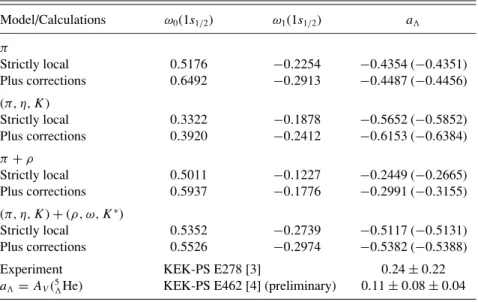
TABLE I. Results for the asymmetry parameter,a, based on the nonmesonic decay
of5
He. See text for detailed explanation.
Model/Calculations ω0(1s1/2) ω1(1s1/2) a
π
Strictly local 0.5176 −0.2254 −0.4354 (−0.4351) Plus corrections 0.6492 −0.2913 −0.4487 (−0.4456) (π, η, K)
Strictly local 0.3322 −0.1878 −0.5652 (−0.5852) Plus corrections 0.3920 −0.2412 −0.6153 (−0.6384) π+ρ
Strictly local 0.5011 −0.1227 −0.2449 (−0.2665) Plus corrections 0.5937 −0.1776 −0.2991 (−0.3155) (π, η, K)+(ρ, ω, K∗)
Strictly local 0.5352 −0.2739 −0.5117 (−0.5131) Plus corrections 0.5526 −0.2974 −0.5382 (−0.5388)
Experiment KEK-PS E278 [3] 0.24±0.22
a=AV(5He) KEK-PS E462 [4] (preliminary) 0.11±0.08±0.04
relation
[Yk(θp, φp)⊗YK(θP, φP)]∗κµ
=(−)k+K−κ+µ[Y
k(θp, φp)⊗YK(θP, φP)]κ−µ. (40) Then, recalling that any spherical harmonic with azimuthal angle equal to, either 0, orπ, is real, one gets
[Yk(θp, π)⊗YK(θP,0)]κ0
=(−)k+K−κ[Y
k(θp, π)⊗YK(θP,0)]κ0, (41)
from which the third one of Eqs. (39) follows immediately. The presence of the phase factori−l′−L′−l−L
in Eq. (38) may seem disquieting at first sight. However, by taking the complex conjugate of that equation, interchanging the dummy variables lLλJ T ↔l′L′λ′J′T′, and making use of Eqs. (39) and of the symmetry properties of angular-momentum coupling and recoupling coefficients, one easily gets the relationω∗
κ =ωκ, showing that these quantities are real, as they should be by definition.
To compute the two-body matrix elements defined in Eq. (29), we resort to a Moshinsky transformation [21] of the initial state, and phenomenologically add initial and final short-range correlations. (For more detail on this and related points, see Refs. [7] and [8].) For5He, the sole contribution to Eq. (38) comes from the 1s1/2proton state, and one can put
L=L′=K=0. On the other hand, for12
C, also the 1p3/2
state contributes, in which caseL andL′ can each take the values 0 and 1. Consequently one could, in principle, have K=0,1 and 2 in Eq. (38). But we prove in Appendix A that the contribution withK =2 vanishes identically, both for κ =0, and forκ =1. Similarly, we prove in Appendix B that the contribution with K=1 vanishes forκ=0. We do not have an analytical proof that the contribution withK=κ =1 vanishes, but we show in Appendix C that it is, in any case, negligibly small. Therefore, only the term withK=0 survives in Eq. (38), and it reduces to the following expression, that can
be used for the two hypernuclei: ωκ =(−)κ
8
√
2πκˆ −1
jp
dcosθp1
dFjpYκ0(θp,0)
×
T T′
(−)T+T′ LS
lλJ
l′λ′J′
il−l′(−)λ+λ′+S+L+jp+12
×lˆlˆ′λˆλˆ′Jˆ2Jˆ′2(l0l′0|κ0)
×
κ 1/2 1/2
jp J J′
κ J′ J S λ λ′
l′ l κ λ λ′L
×M(plP LλSJ T;jjp)M∗(pl′P Lλ′SJ′T′;jjp), (42) withL=0 for the 1s1/2state, andL=0 and 1 for the 1p3/2
state.
It is interesting to observe that the presence of the Clebsch-Gordan coefficient in Eq. (42), for κ=1, ensures that landl′ have opposite parities. Since the initial state in the two matrix elements has a definite parity, this implies that all contributions to ω1 come from interference terms
between the parity-conserving and the parity-violating parts of the transition potential. Furthermore, the antisymmetrization factor in Eq. (29) shows that the two final states haveT =T′. These are general properties of the asymmetry parameter, as mentioned in the introduction.
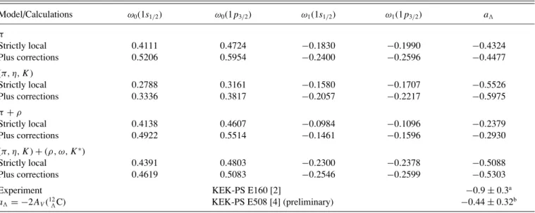
V. NUMERICAL RESULTS AND CONCLUSIONS Shown in Tables I and II are the results obtained in the calculation of the asymmetry parameter, a, based on the expressions of the previous section applied to5
He and12C, respectively. The values ofω0 andω1are in units of the free
decay constant, Ŵ(0)=2.50×10⁻⁶ eV, and, in the case
of12
C, we give in separate columns the contributions of the 1s1/2and 1p3/2proton states. Also included are the measured
TABLE II. Results for the asymmetry parameter,a, based on the nonmesonic decay of12C. See text for detailed explanation.
Model/Calculations ω0(1s1/2) ω0(1p3/2) ω1(1s1/2) ω1(1p3/2) a
π
Strictly local 0.4111 0.4724 −0.1830 −0.1990 −0.4324
Plus corrections 0.5206 0.5954 −0.2400 −0.2596 −0.4477
(π, η, K)
Strictly local 0.2788 0.3161 −0.1580 −0.1707 −0.5526
Plus corrections 0.3336 0.3817 −0.2057 −0.2217 −0.5975
π+ρ
Strictly local 0.4138 0.4607 −0.0984 −0.1096 −0.2379
Plus corrections 0.4922 0.5514 −0.1461 −0.1596 −0.2930
(π, η, K)+(ρ, ω, K∗)
Strictly local 0.4391 0.4803 −0.2300 −0.2378 −0.5088
Plus corrections 0.4619 0.5083 −0.2546 −0.2599 −0.5303
Experiment KEK-PS E160 [2] −0.9±0.3a
a= −2AV(12C) KEK-PS E508 [4] (preliminary) −0.44±0.32
b
aThis result corresponds to an improved weighted average among severalp-shell hypernuclei [1, p. 95]. bSee text.
in12C extracted from experiment KEK-PS E508 and given in Table II was taken from the preprint version of Ref. [4], since only a weighted average for12
C and11B is explicitly reported in the published version, its value being−0.20±0.26±0.04. We consider several OME models, and for each one we give the results of two different calculations. First are those corresponding to the strictly local approximation for the transition potential, usually adopted in the literature. Second are the ones obtained when we add the corrections due to the kinematical effects related to the lambda-nucleon mass difference and the first-order nonlocality terms that we have discussed in Ref. [8]. The first thing to notice is that these corrections act systematically in the direction of increasing the absolute values of all the tabulated quantities. The effect is typically in the range of 20–30% forωκbut only 5–10% for a, tending to be larger in theπ+ρmodel and smaller in the complete model. To put it shortly, if one wants precise values for the asymmetry parameter, the correction terms should be included in the transition potential, but, in view of the present level of indeterminacy in the measurements, they can be dispensed with for the moment.
In the case of 5He, we have also included, between parentheses, in Table I, the values fora obtained with the approximate formula usually adopted in the literature [1], namely,
AV
5
He
≈ 2ℜ[
√
3ae∗−b(c∗−√2d∗)+√3f(√2c∗+d∗)]
|a|2+ |b|2+3(|c|2+ |d|2+ |e|2+ |f|2) ,
(43) where
a=np,1S0
V
p,1S0
, b=inp,3P0
V
p,1S0
,
c=
np,3S1
V
p,3S1, d = −np,3D1
V
p,3S1,
e=i
np,1P1
V
p,3S1, f = −inp,3P1
V
p,3S1.
(44)
The extra factors in the transition amplitudes in Eqs. (44) are due to differences in phase conventions, as explained in Ref. [8]. It is important to emphasize that Eq. (43) is only an approximation, that can be adapted from the corresponding expression for the two-body reaction pn→p in free space [22]. As such, it ignores the fact that the final state of nonmesonic decay is a three-body one and the ensuing kine-matical complications should be properly dealt with, which requires a direct integration over the available phase space as done in the expressions used here. More importantly, Eq. (43) does not include the full contribution of the transitions coming from proton states beyond thes-shell, being therefore of only limited validity, and should not be used forp-shell hypernuclei such as12
C, or, even worse, for heavier ones. This being said, comparison of the corresponding values forain Table I shows that the formula works well within its range of validity. This conclusion is in agreement with our preliminary result reported elsewhere [23], which was restricted to one-pion-exchange only.
Coming now to12
C, it is evident in Table II that thep-shell contributions toω0andω1 are by no means negligible, being
in fact of the same order as those of thes-shell. However, they are also in approximately the same ratio, so that the effect on a, given by Eq. (37), is much smaller. This corroborates the theoretical expectation that the intrinsic asymmetry parameter, a, should have only a moderate dependence on the particular hypernucleus considered. Presently we are investigating to which degree this remains true for more general cases, such as that of11
B [24]. Notice that in the previous section we have explicitly proven thata is independent of the hypernuclear spin. However this does not, by itself, exclude the possibil-ity that it might depend on other aspects of hypernuclear structure.
treat the contribution of transitions originating from proton states beyond the s-shell. As to our numerical results, let us first of all observe that the calculated values of a in the four OME models considered here vary from −0.62 to −0.24. This broad spectrum of values indicates that the asymmetry parameter can indeed be a powerful tool to discriminate between different theoretical mechanisms for nonmesonic decay, requiring for this purpose, however, a more precise experimental determination of this observable than those presently available. Secondly, the fact that, for each of these OME models, the results for5
He and12C are very similar is compatible with the general expectation that a should depend little on the hypernucleus. Finally, the negative value systematically obtained fora for the two hypernuclei indicates, once again, that it will be hard to get a positive or zero value for it in the first case, at least within strict OME models. The puzzle posed by the experimental results fora ins- andp-shell hypernuclei remains unexplained.
APPENDIX A:K=2 CONTRIBUTIONS TOω0ANDω1
As mentioned in Sec. IV, to compute the transition matrix elementsMappearing in Eq. (38), we perform a Moshinsky transformation of the initialpstate ([8] Eq. (A.1)),
|jjpJ)=jˆjˆp
¯
λS¯ ˆ¯ λSˆ¯
l 1/2j lp 1/2jp
¯ λ S¯ J
×
n¯lN L
(nlN L¯ λ¯|nlnplpλ)¯ |nlN L¯ λ¯SJ)¯
≡
nlN L¯ λ¯S¯
C(nlN L¯ λ¯S;¯ jjpJ)|nlN L¯ λ¯SJ),¯ (A1)
where (nlN L¯ λ¯|nlnplpλ) are the Moshinsky brackets with¯ their phases adapted so as to conform with our convention for the relative coordinate as discussed in Appendix A of Ref. [8]. We have put bars over ¯l,λ¯ and ¯Sto distinguish them from the analogous angular momenta in the partial waves of the final NN state. This is not necessary forL andJ, since all transitions are diagonal in these two quantum numbers. Introducing Eq. (A1) into Eq. (29), one gets
M(plP LλSJ T;jjp)
=
n¯lNλ¯S¯
C(nlN L¯ λ¯S;¯ jjpJ)M(plP LλSJ T;nlN¯ λ¯S),¯ (A2)
where
M(plP LλSJ T;nlN¯ λ¯S)¯
= √1
2[1−(−)
l+S+T](plP LλSJ T
|V|nlN L¯ λ¯SJ¯ ). (A3)
The transition potential can be decomposed as
V =
i
vi(r)Iii, (A4)
where the isospin factor Ii is equal to 1 or τ1·τ2, for isoscalar or isovector interactions, respectively, and the i are rotationally invariant operators having definite spin and spatial ranks, i.e., operators of the form
i = Aνii(σ1,σ2)⊗Bνi i (r,∇)
00. (A5)
Due to the algebraic properties of the Pauli matrices, the rank νican be at most equal to 2. For the OME models we consider, including eventual kinematical and nonlocality corrections, the several possibilities are
PC terms
νi =0 for central andr· ∇forces (spin-independent or spin-spin), νi =1 for linear spin-orbit forces, νi =2 for tensor forces;
PV terms{νi=1 for all kinds. (A6) As can be seen in Eqs. (A.3) to (A.15) of Ref. [8], the different terms have matrix elements of the general form
(plP LλSJ T|viIii|nlN L¯ λ¯SJ¯ )
=Gi(lLλSJ T; ¯lλ¯S)(P L¯ |N L)(pl|vi(r) ˆdi(r)|nl),¯ (A7) where (P L|N L) are the overlaps of the c.m. radial wave functions and the ˆdi(r) are, either unity, or one of the effective differential operators defined in Eq. (A.16) of that reference. The important point is that the Gi are purely geometrical factors, involving, at most, 3j and 6j symbols. Scrutinizing these equations more closely, one notices that the dependence onλ,λ¯ andJcan be isolated as follows:
Gi(lLλSJ T; ¯lλ¯S)¯ =(−)Jλˆˆ¯λ
λ ν
i λ¯ ¯ l L l
λ ν
i λ¯ ¯ S J S
gi(lLST; ¯lS).¯ (A8) This result is completely general and depends only on the application of the Wigner-Eckart theorem to operators of the form given in Eq. (A5). (See, for instance, Chap. 7 of Ref. [25], or Sec. 1A-5 of Ref. [26].)
Taking these ideas into account in Eq. (38), it is clear that the summation overλ, J, λ′ and J′ can be performed first, leading to a remaining summand that is proportional to
λJ
λ′J′
(−)λ+J+J′ˆ
λ2λˆ′2Jˆ2Jˆ′2
×
κ 1/2 1/2 jp J J′
κ J′ J S λ λ′
l l′ k L L′K λ λ′ κ
×
l1/2j lp 1/2 jp
¯ λ S¯ J
λ ν
i λ¯ ¯ l L l
λ νi λ¯ ¯ S J S
×
l 1/2j lp 1/2 jp
¯ λ′ S¯′ J′
λ′ν
i′ λ¯′ ¯ l′ L′ l′
λ′ν i′ λ¯′ ¯ S′J′ S
Actually, theis always in the 1s1/2state, and one can make
use of Eq. (6.4.14) of Ref. [25] to replace the above expression by
X≡
λJ
λ′J′
(−)λ+J+J′λˆ2λˆ′2Jˆ2Jˆ′2
×
κ 1/2 1/2
jp J J′
κ J′J S λ λ′
l l′ k L L′K λ λ′ κ
× S¯ 1/2 1/2 jp lp J
λ νi lp ¯ l L l
λ νi lp ¯ S J S
×
S¯′ 1/2 1/2
jp lp J′ λ′ν
i′lp ¯ l′ L′ l′
λ′ν i′lp ¯ S′J′ S
, (A10) where we have dropped an irrelevant factor.
For a proton in thesshell, the Moshinsky transformation requires that L=L′=0, and the 9j symbol in Eq. (A10) selectsK=0 as the only possibility. For a proton in the p
shell, there are two alternatives for the relative and c.m. angular momenta, namely,
pshell
alternative 1: ¯l=1 andL=0,
alternative 2: ¯l=0 andL=1, (A11) and similarly for the primed quantities. In principle, therefore, there are three possibilities forK, namely,K=0,1 and 2.
It is clear from this discussion that a contribution with K=2 in Eq. (38) can only come from the alternative 2 in Eq. (A11). Therefore, setting L=L′=1 and ¯l =l¯′=0 in Eq. (A10), and making use of Eq. (6.3.2) of Ref. [25], we get
X
jp =1pjp;L=L
′=1
=(−)
l+l′
3ˆllˆ′ δνilδνi′l′
λJ
λ′J′
(−)λ′+J+J′ˆ
λ2λˆ′2Jˆ2Jˆ′2
×
κ 1/2 1/2 jp J J′
κ J′ J S λ λ′
l l′ k 1 1K λ λ′ κ
×
S¯ 1/2 1/2
jp 1 J
λ l 1 ¯ S J S
×
S¯′1/2 1/2
jp 1 J′
λ′ l′ 1 ¯ S′J′S
. (A12)
To proceed, it will be unavoidable to perform some manipulations with 12j symbols, and the needed identities are collected in Appendix D for convenience. With the help of well-known symmetry properties of 6j and 9j symbols [25], one can make use of Eqs. (D2), (D3), and (D4), in succession, to perform, first the summation overλ, and then that overλ′, in Eq. (A12), getting
Xjp =1pjp;L=L
′=1
= (−)
K+l′+S¯′
3ˆllˆ′ δνilδνi′l′
k S¯ S¯′
S l′ l
×
J
J′ (−)J′ ˆ
J2Jˆ′2
k S¯ S¯′ κ J J′ K 1 1
×
κ 1/2 1/2
jp J J′ ¯
S 1/2 1/2 jp 1 J
× S¯′
1/2 1/2 jp 1 J′
. (A13)
Repeating the same procedure, we can now perform, first the summation overJ, and then that overJ′, to get
X
jp =1pjp;L=L
′
=1
= −(−)
K+k+l′+S¯′
3ˆllˆ′ δνilδνi′l′
kS¯S¯′ S l′ l
×
K1/2 1/2 κ 1/2 1/2 k S¯ S¯′
K1/2 1/2
jp 1 1
. (A14)
The 9j, as well as the last 6j, in Eq. (A14) restrictsKto 0 and 1, and we conclude that the contribution withK=2 in Eq. (38) vanishes identically, both forκ =0, and forκ =1. Notice that this result holds, not only forjp =1p3/2, which is
of direct interest for12
C, but also forjp =1p1/2, which may
be relevant for otherp-shell hypernuclei.
APPENDIX B:K=1 CONTRIBUTION TOω0
Recalling Eq. (33), it is clear that theK=1 contribution toω0in Eq. (38), from the single-proton statejp, has the form
ω0(jp, K=1)=
dcosθp1
p22dp2
p21dp1
×δ
p2
1
2M+ p22 2M+
|p1+p2|2
2MF −
jp
×f(p, P)[Y1(θp, π)⊗Y1(θP,0)]00, (B1)
wheref(p, P) represents the rest of the integrand in Eq. (38), the important point being that it depends on the momenta only throughpandP.
From the explicit expressions of the spherical harmonics, we find
[Y1(θp, π)⊗Y1(θP,0)]00= −
√
3
4π cos(θp+θP), (B2) and, making use of the last two equations in Eq. (15), this becomes
[Y1(θp, π)⊗Y1(θP,0)]00= −
√
3 4π
p22−p21
2pP . (B3)
Introducing this result in Eq. (B1), we are left with ω0(jp, K =1)= −
√
3 4π
dcosθp1
p22dp2
p21dp1
×δ
p2
1
2M+ p22 2M+
|p1+p2|2
2MF −
jp
×f(p, P)p
2 2−p21
2pP . (B4)
Let us now perform the interchange of dummy variablesp1↔
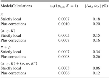
TABLE III. Results for the K=1 contribution to ω1 in the nonmesonic decay of12
C. See text for detailed explanation.
Model/Calculations ω1(1p3/2, K=1) |a/a|(%)
π
Strictly local 0.0007 0.18
Plus corrections 0.0010 0.20
(π, η, K)
Strictly local 0.0005 0.15
Plus corrections 0.0007 0.16
π+ρ
Strictly local 0.0007 0.34
Plus corrections 0.0008 0.26
(π, η, K)+(ρ, ω, K∗)
Strictly local 0.0003 0.06
Plus corrections 0.0006 0.12
according to the first two equations in Eq. (15),pandPare invariant under this transformation, we arrive at the result
ω0(jp, K=1)= −ω0(jp, K=1), (B5) from which it follows that the contribution with K=1 in Eq. (38) vanishes forκ =0.
APPENDIX C:K =1 CONTRIBUTION TOω1
We have not been able to find an analytical proof that the K=1 contribution in Eq. (38) vanishes also forκ =1. However, for the cases we are dealing with, this contribution can only arise from the jp =1p3/2 proton state in 12C, and we have numerically computed its values in the several OME models we are considering. They are given, in units ofŴ(0), in Table III. The nonzero values may be due to truncation and roundoff errors. For instance, we have computed, with the same routine, the analogous contribution withκ =0 in the case of the complete OME model plus kinematical and nonlocality terms. Even though it has been proved in Appendix B that this is exactly zero, the numerical result came out as 0.0004, which is comparable to the value obtained forω1(1p3/2, K=1) in
the same model.
Comparison of Tables II and III immediately shows that the K=1 contribution to ω1 is, in any case, very small.
Furthermore, in the last column of Table III, we give the relative
effect that its inclusion would have ona, and it always stays below 0.4%. We conclude that, even if this contribution is not exactly zero, it can be safely neglected.
APPENDIX D: SOME PROPERTIES OF 12jSYMBOLS The 12j symbols arise in the recoupling of five angular momenta [27,28]. They are not unique, but here we shall need only those of the first kind,
j1 j2 j3 j4
l1 l2 l3 l4
k1 k2 k3 k4
=
x
(−)R4−xxˆ2
× j
1 k1 x
k2 j2 l1
j2 k2 x
k3 j3 l2
j3 k3 x
k4 j4 l3
j4 k4 x
j1 k1 l4
, (D1) as defined in Eq. (19.1) of Ref. [28], whose notation for the 12jsymbols we follow. In Eq. (D1),R4stands for the sum of
all the angular momentum labels in the 12j symbol.
These symbols obey the recursion relation ([28], Eq. (A.6.13))
j1 j2 j3 j4
l1 l2 l3 l4
k1 k2 k3 k4
=(−)j2+k2+j4+k4
×
x
(−)2xxˆ2
k2 j4 x
l2 j3 j2
k3 l3 k4
k
2 j4 x
l4 l1 k1
k4 j2 x
l1 l4 j1
, (D2)
and have several symmetry properties, among which ([28] Eq. (17.4))
j1 j2 j3 j4
l1 l2 l3 l4
k1 k2 k3 k4
=
j2 j3 j4 k1
l2 l3 l4 l1
k2 k3 k4 j1
. (D3)
There are also reduction formulas, such as ([28] Eq. (A.6.39)),
x ˆ x2
j1 j2 j3 j4
l1 l2 l3 l4
x k2 k3 k4
l
1 k2 x
j4 l4 k1
=(−)l2+l3+j3+k3−k1
j2k4k1
j3 l3 j4
l2 k3k2
j
2k4k1
l4 l1 j1
. (D4)
[1] W. M. Alberico and G. Garbarino, Phys. Rep.369, 1 (2002). [2] S. Ajimuraet al., Phys. Lett.B282, 293 (1992).
[3] S. Ajimuraet al., Phys. Rev. Lett.84, 4052 (2000).
[4] T. Marutaet al., Nucl. Phys.A754, 168c (2005); see also nucl-ex/0402017.
[5] J. F. Dubach, G. B. Feldman, B. R. Holstein, and L. de la Torre, Ann. Phys. (NY)249, 146 (1996).
[6] A. Parre˜no, A. Ramos, and C. Bennhold, Phys. Rev. C56, 339 (1997); A. Parre˜no and A. Ramos,ibid.65, 015204 (2002).
[7] C. Barbero, D. Horvat, F. Krmpoti´c, T. T. S. Kuo, Z. Naranci´c, and D. Tadi´c, Phys. Rev. C66, 055209 (2002).
[8] C. Barbero, C. De Conti, A. P. Gale˜ao, and F. Krmpoti´c, Nucl. Phys.A726, 267 (2003).
[10] K. Sasaki, T. Inoue, and M. Oka, Nucl. Phys.A707, 477 (2002); A669, 331 (2000); Erratum,ibid.A678, 455 (2000).
[11] G. Garbarino, A. Parre˜no, and A. Ramos, Phys. Rev. C 69, 054603 (2004), and references therein.
[12] W. M. Alberico, G. Garbarino, A. Parre˜no, and A. Ramos, Phys. Rev. Lett.94, 082501 (2005).
[13] A. Ramos, E. van Meijgaard, C. Bennhold, and B. K. Jennings, Nucl. Phys.A544, 703 (1992).
[14] A. Parre˜no, C. Bennhold, and B. R. Holstein, Phys. Rev. C70, 051601(R) (2004).
[15] K. Sasaki, M. Izaki, and M. Oka, Phys. Rev. C 71, 035502 (2005).
[16] H. Ejiri, T. Fukuda, T. Shibata, H. Band¯o, and K.-I. Kubo, Phys. Rev. C36, 1435 (1987).
[17] N. Austern, Direct Nuclear Reaction Theories (Wiley-Interscience, New York, 1970).
[18] A. P. Gale˜ao (in preparation).
[19] A. P. Gale˜ao, in IX Hadron Physics and VII Relativistic Aspects of Nuclear Physics: A Joint Meeting on QCD and QGP, Rio de Janeiro, 28 March–3 April 2004, edited by M. E. Bracco, M. Chiapparini, E. Ferreira, and T. Kodama, AIP Conf. Proc.
No. 739, 560 (2004), see also extended version mentioned therein.
[20] F. Krmpoti´c and D. Tadi´c, Braz. J. Phys.33, 187 (2003). [21] M. Moshinsky, Nucl. Phys.13, 104 (1959).
[22] H. Nabetani, T. Ogaito, T. Sato, and T. Kishimoto, Phys. Rev. C 60, 017001 (1999).
[23] C. Barbero, A. P. Gale˜ao, and F. Krmpoti´c, Braz. J. Phys.34, 822 (2004).
[24] C. Barbero, A. P. Gale˜ao, and F. Krmpoti´c, work in progress. [25] A. R. Edmonds, Angular Momentum in Quantum Mechanics
(Princeton University Press, Princeton, NJ, 1974).
[26] A. Bohr and B. R. Mottelson, Nuclear Structure, Vol. I (Benjamin, Inc., New York, 1969).
[27] M. Rotenberg, R. Bivins, N. Metropolis, and J. K. Wooten Jr.,
The 3-j and 6-j Symbols(The Technology Press, MIT, Cam-bridge, MA, 1959).