MESTRADO EXECUTIVO EM GESTÃO EMPRESARIAL
ANALYTICAL ANALYSIS OF CONSUMPTION IN
BRAZIL
GRETA BUTVILAITE
Rio de Janeiro - 2016MESTRADO EXECUTIVO EM GESTÃO EMPRESARIAL
ANALYTICAL ANALYSIS OF CONSUMPTION IN
BRAZIL
GRETA BUTVILAITE
Rio de Janeiro - 2016DISSERTAÇÃO APRESENTADA À ESCOLA BRASILEIRA DE ADMINISTRAÇÃO
PÚBLICA E DE EMPRESAS PARA OBTENÇÃO DO GRAU DE MESTRE
Butvilaite, Greta
Analytical analysis of consumption in Brazil / Greta Butvilaite. – 2016. 61 f.
Dissertação (mestrado) - Escola Brasileira de Administração Pública e de Empresas, Centro de Formação Acadêmica e Pesquisa.
Orientador: Fabio Caldieraro. Inclui bibliografia.
1. Consumo (Economia) – Brasil. 2. Análise por conglomerados. 3. Pesquisa de mercado. I. Caldieraro, Fabio. II. Escola Brasileira de Administração Pública e de Empresas. Centro de Formação Acadêmica e Pesquisa. III. Título.
ABSTRACT
This thesis is an analytical analysis of consumption in Brazil, based on data from the
Consumer Expenditure Survey, years 2008 to 2009, collected by the Brazilian Institute of
Geography and Statistics. The main aim of the thesis was to identify differences and similarities
in consumption among Brazilian households, and estimate the importance of demographic and
geographic characteristics.
Initially, households belonging to different social classes and geographical regions were
compared based on their consumption. For further insights, two cluster analyses were conducted.
Firstly, households were grouped according to the absolute values of expenditures. Five clusters
were discovered; cluster membership showed larger spending in all of the expense categories for
households having higher income, and a substantial association with particular demographic
variables, including as region, neighborhood, race and education. Secondly, cluster analysis was
performed on proportionate distribution of total spending by every household. Five groups of
households were revealed: Basic Consumers, the largest group that spends only on fundamental
goods, Limited Spenders, which additionally purchase alcohol, tobacco, literature and
telecommunication technologies, Mainstream Buyers, characterized by spending on clothing,
personal care, entertainment and transport, Advanced Consumers, which have high relative
expenses on financial and legal services, healthcare and education, and Exclusive Spenders,
households distinguished by spending on vehicles, real estate and travelling.
TABLE OF CONTENTS
1 INTRODUCTION ... 8
1.1 Contextualization and relevance of the problem ... 8
1.1.1 Size and growth of the Brazilian consumer market ... 8
1.1.2 Sophistication of consumer market ... 9
1.2 Justification of the theme selection ... 10
1.3 Structuring of the paper ... 11
2 PROBLEM TO BE DISCUSSED ... 12
2.1 Research question and objectives ... 12
2.2 Limits of the research problem ... 12
2.3 Expected results ... 13
3 THEORETICAL REFERENCE ... 14
4 RESEARCH METHOD ... 16
4.1 Data source ... 16
4.1.1 Specification and research design ... 17
4.1.2 Currency ... 18
4.1.3 Purpose ... 18
4.1.4 Content ... 19
4.1.5 Dependability ... 21
4.2 Data analysis process ... 21
5 DATA ANALYSIS ... 23
5.1 Data preparation ... 23
5.2 Data analysis ... 24
5.2.1 Overview of the sample ... 24
5.2.2 General consumption patterns ... 28
5.2.3 Clustering by absolute values ... 32
5.2.4 Clustering by percentile amount ... 37
6 MAIN FINDINGS ... 46
6.1 Overview of results ... 46
6.2 Conclusions ... 47
6.4 Recommendations for future research ... 50
APPENDIX ... 52
6.5 Appendix A ... 52
6.6 Appendix B ... 54
List of Figures
Figure 1. Location of POF survey respondents. Displayed by region, geographical area
(urban or rural), and state. ... 25
Figure 2. Respondents by age and gender of the reference person. ... 27
Figure 3. Ownership of credit cards and health insurance. ... 27
Figure 4. Composition of total expenses. ... 28
Figure 5. Total expenses by social class. ... 29
Figure 6. Social classes by size and total spending. ... 30
Figure 7. Regions by average monthly income per household. ... 31
Figure 8. Regions by average monthly income per household. ... 31
Figure 9. Means of expenditures by each cluster. ... 33
Figure 10. Clusters by size and total spending (clustering by absolute amounts). ... 37
Figure 11. Differences in expense groups by clusters (clustering by absolute amounts). . 40
Figure 12. Clusters by size and total spending (clustering by percentile amounts). ... 44
Figure 13. Composition of Brazilian society and predicted changes. ... 49
List of Tables
Table 1. Social classes: mean income, size, portion of total income ... 26Table 2. Demographic descriptors of clusters (clustering by absolute amounts) ... 34
Table 3. Means of percentile expenditures in every category, by clusters ... 39
LIST OF SYMBOLS, ABBREVIATIONS AND ACRONYMS
ANS – Agência Nacional de Saúde Suplementar (Eng. The National Regulatory Agency for Private Health Insurance and Plans)
GDP – General Domestic Product
IBGE – Instituto Brasileiro de Geografia e Estatística (Eng. Brazilian Institute of Geography and Statistics)
SAE/PR - A Secretaria de Assuntos Estratégicos da Presidência da República (Eng. Strategic Affairs Secretariat)
1
INTRODUCTION
1.1 Contextualization and relevance of the problem
In the last decade, Brazil has been continuously listed as a destination of opportunities and
growth. Even in current times of political instability and economical struggles, Brazil remains the
7th largest economy in the world, and an important international trade partner (IMF, 2015;
Lamucci, 2015).
Besides its size, what makes Brazil an attractive destination for business? Such question
neither could nor shall be answered right away. Countless models were created to help evaluate
and prioritize different markets based on their accessibility, potential, strategic fit and numerous
other variables. Among all determinants, most of the authors give major importance to the market
itself – its consumer base. Therefore, the focus of this paper is on the demand conditions –
Brazilian consumers.
To provide the context of Brazilian consumer market, it is assessed by its size, growth and
sophistication.
1.1.1 Size and growth of the Brazilian consumer market
Admittedly, Brazil is one of the biggest markets in the world. It has the 5th largest
population worldwide of over 205 million that is predominantly young - around 44.6% of the
population are aged from 15 to 43 of all the people aged over 15, as of year 2013 (Euromonitor
International, 2014) (World Bank, 2015).
The amount of Brazilians actively participating in the consumer market has increased
greatly throughout the last decade, mostly due to growth of the middle class. Numerous factors
contributed to this change, including both – favorable market conditions and governmental
policies. (World Bank, 2015)
Regarding market conditions, rising demand for low-skilled workers resulted in higher
wages, and in turn boosted the disposable income of consumers, which was especially noticeable
in the poorest parts of society. Clearly, such increase in disposable income of Brazilians has been
partly a result of public policies. (World Bank, 2015)
Firstly, Brazilian government augmented investments into education, which lead to better
job opportunities and thus higher salaries. Moreover, extensive cash transfer programs, including
Familia, were introduced in the beginning of the century, aimed to decrease poverty and fight
inequality. Bolsa Familia has been supporting around 50 million Brazilians with conditional cash
transfers, and is considered to be one of the most important reducers of poverty and income
inequality. Amount of people in poverty fell from 24.9% in 2001 to 8.9% in 2013, which added
up to around 25 million people entering the middle class. In addition, GINI index, a measure of
income inequality in the country, fell by around 11%, suggesting significant improvements in
narrowing the income gap. Such changes are reflected in the composition of the Brazilian society:
according to the World Bank, around 70% of Brazilians, 144 million people, belong to the middle
class, which is contributing over the half of the whole consumer spending. (World Bank, 2015)
(Özler, 2014)
Together with rising disposable income, Brazilian consumers are spending increasing
amounts due to access to debt financing: customer credit has become easily attainable and
frequently used among Brazilian consumers. As of December, 2014, consumers’ debt in Brazil
amounts to the level corresponding to around 15% of country’s Gross Domestic Product (GDP).
This debt has been growing in the last decade: August of 2015 shows an 8% increase from the
corresponding month last year. Customers admit to be very inclined to buy with installments and
take out loans, which again enhances the scale of consumption. (Banco Central do Brasil, 2015)
(World Bank, 2015) (Chao & Lyons, 2013)
Realizing their growing ability to purchase, Brazilians are showing a high inclination to
actually spend their income on consumer goods. Among Brazilian middle class, abundance of
purchases is commonly considered to be a symbol of financial success and high social status.
According to a research conducted by McKinsey & Company, 46% of Brazilians see shopping as
one of the most pleasant pastimes with their family. That being so, Brazilian consumers are
spending more than investing; personal liabilities have been increasing more rapidly than assets.
(McKinsey & Company, 2015)
1.1.2 Sophistication of consumer market
According to Michael Porter, quality of the market may be more important than its size
(Porter, 1998). Brazilian consumers are not considered to be highly sophisticated: instead of
creating needs, they rather follow foreign trends. However, Brazilian consumers’ needs, wants
and sophistication have been evolving substantially. A decade ago, majority of customers aspired
been shifting from focusing on alimentation to durable goods, leisure activities and more
exclusive products. Industries that have been increasingly growing are education, beauty products
and services, plastic surgery and apparel. One of the most prominent trends contributing to
advancement of Brazilians is internet and mobile connectivity, which has shown a significant
increase: according to World Bank, the amount of Brazilians using the internet and having a
mobile subscription increased by 70% and 76% respectively since 2003. This implies that
consumers can research and compare goods before buying, are connected to current affairs and
influences from social networks. (World Bank, 2015) (McKinsey & Company, 2015)
Even though the answer varies company to company, generally, an attractive market
offers space for growth by its large scale, promising future by its high growth rates, push for
innovation by its sophistication, and an opportunity to differentiate by its heterogeneity. The
latter, analysis of the differences and similarities of Brazilian consumers, is chosen to be the
focus of this thesis. (Porter, 1998; Shane, 2004)
1.2 Justification of the theme selection
Analyzing consumption in Brazil was found to be important and thus chosen as the focus
of this thesis for following reasons.
Firstly, as discussed in section 1.1 Contextualization and relevance of the topic, Brazilian
consumer market is one of the biggest worldwide and is predicted to have an increasing
importance in the future. Therefore, understanding Brazilian consumers is necessary in order to
be successful in a global business context: fruitful consumer prioritization and targeting requires
a thorough analysis of characteristics of the Brazilian market. With this paper, it is aimed to
analyze and split Brazilian consumers into groups sharing similar consumption patterns.
Therefore, this thesis would be a potential source of marketing intelligence for interested entities.
Secondly, Institute Brasileiro de Geografia e Estatística (IBGE) created an excellent
source of information regarding Brazilian consumption, involving almost 60 thousand residents.
Even though IBGE has published its conclusions and commentary, extent of data allows
alternative, yet unexplored approaches to analysis. Therefore, with this thesis it is expected to
utilize the survey to reveal additional insights.
Thirdly, IBGE is conducting the Consumer Expenditure Survey periodically, thus the
approach to research and analysis techniques employed could be replicated in the future. In this
1.3 Structuring of the paper
This paper is organized in the following manner. After introducing the topic with context
overview and explanation of its relevance, the main research question, general and specific
objectives are discussed. The part is followed by limitations of the research question and
description of expected results.
In order to establish the state of dialogue for the chosen topic, relevant publications are
reviewed. Subsequently, the chosen research method is discussed, including the approach to
research, a thorough overview of the main sources of information, and the process of data
analysis.
Afterwards, data analysis is described. Firstly, data preparation process is explained in
detail. Secondly, the sample of the survey is overviewed, as well as general consumption patterns
in Brazil, including differences in consumption by households belonging to different social
classes and residing in various locations throughout the country. Afterwards, two cluster analyses
are performed: based on absolute and percentile values of expenditures.
The main results are overviewed followed by core conclusions, limitations assumed and
2
PROBLEM TO BE DISCUSSED
2.1 Research question and objectives
The main research question of the paper is the following: how does consumer spending in
Brazil vary, and to which extent depend on demographic and geographic characteristics of
consumers?
The general objective of the thesis is to discover and understand the heterogeneity of
consumer spending in Brazil.
The main specific objectives of the thesis are formulated in the following manner:
1. To overview the core characteristics of Brazilian consumers
2. To reveal the main consumption patterns of Brazilian households belonging to
different social classes and residing in diverse areas throughout the country
3. To discover significant differences and similarities among households from two
perspectives: based on their total expenditures and proportional distribution of
expenditures
4. Group households into meaningful clusters based on their consumption patterns
5. Reveal to which extent cluster members share the same demographic and geographic
characteristics
As an additional intention, this thesis should provide a framework for future analysis of
consumption patterns in Brazil when new data becomes available. Therefore, research approach
employed in this paper should be designed in a way that it can be replicated in the future.
2.2 Limits of the research problem
Limits of the research problem are mostly concerned with a low level of specificity of the
analysis. Since the analysis is not conducted exclusively for a particular company or industry,
results might turn out to be overly general to be applied on an individual basis. That being so, this
thesis does not aim to be the only guiding source of information for a certain interested party.
Instead, the purpose of the paper is to provide general insights on the Brazilian consumer market
2.3 Expected results
Firstly, it is expected to overview Brazilian consumer market, emphasizing the most
prominent demographic characteristics as well as destinations of expenses and overall level of
spending.
Secondly, it is expected to find differences and similarities in consumption across
geographical regions of Brazil. Variations are expected across rural and urban areas, as well as
different parts of the country. Demographic characteristics are expected to also cause differences
in the way consumers spend their income; income, age and education are thought to have the
most importance.
It is expected to group households into meaningful clusters based on their levels,
destinations and preferences of expenses. In addition, it is aimed to find unexpected similarities
among consumers regarding their consumption yet having different demographic characteristics.
As an overall anticipation, this thesis should be a valuable source for companies operating
or aiming to operate in Brazil. Findings of this paper are expected to give insights on consumer
profiles across different regions, including their demographic characteristics and spending habits.
Such information should be useful in various business processes including market segmentation
3
THEORETICAL REFERENCE
Consumption in Brazil is a constant object of discussion and analysis, covered by multiple
Brazilian and international researchers, consulting companies and various institutions. Usually,
Brazilian consumers are analyzed on an industry-specific basis; in this section, main publications
on Brazilian consumption are overviewed in order to establish the state of dialogue of the topic.
Reports by IBGE. IBGE has published several Consumer Expenditure Survey results and
commentary papers. Publication on Profile of expenditures in Brazil is an extensive collection of
statistics on consumption in Brazil; the chosen approach of IBGE was to present expenses by
selected indicators, for instance, expenses by different age group, gender, area, family
composition and numerous other factors.
Living conditions and sources of income are also largely covered in other publications by
IBGE. In addition, a large part of analysis carried out by IBGE is focused on alimentation of
Brazilians, nutritional differences across the society and changes since the previous consumption
survey.
However, with its analysis IBGE does not aim to group households by their consumption
habits; instead, it seeks to connect individual demographic variables with all kinds of expenses.
(IBGE, 2010)
Reports by consulting companies. Several consulting companies have publicized
analyses of Brazilian consumer market. An important contributor is McKinsey Global Institute,
which has published multiple reports, such as “Connecting Brazil to the world. A path to
inclusive growth” in 2014. This report touched the consumption trends in Brazil, focusing on
exploring how Brazil compares to other countries regarding consumption and multiple other
indicators, including productivity and social development, and providing recommendations to
boost development of Brazil.
In addition, McKinsey and Company has published various briefings regarding different
industries in Brazil, including luxury goods, beauty industry and the e-commerce. (Elstrodt,
Manyika, Remes, Ellen, & Martins, 2014)
Publications by other researchers. Among other entities, Information Service companies
supply extensive information for the interested parties. For instance, Euromonitor International
development, as well as an extensive report on Brazilian consumers’ lifestyles. (Euromonitor
International, 2014, 2015)
There is also a big number of reports conducted by individual researchers analyzing
Brazil on a specific industry product basis, such as biofuel, specific food products, tobacco and
alcohol consumption and various other types of analysis.
All in all, attempts to group Brazilian consumers are frequently based on demographic
characteristics, such as are age, income, region or race of consumers. In addition, Brazilian
consumer market is usually analyzed on an industry or sector basis. Therefore, it was decided that
grouping households by all types of expenses and just afterwards testing for associations between
demographic characteristics and cluster membership would be an interesting and fairly original
4
RESEARCH METHOD
This thesis is a descriptive study on Brazilian consumption, aimed to analyze the main
consumer characteristics and consumption patterns. Below, the main data source is thoroughly
described and justified, followed by an explanation of approach to data analysis.
4.1 Data source
Analysis in this thesis is relies on the secondary data, which refers to information
collected for other purposes than this particular paper, but is considered to be utilizable.
(Malhotra & Birks, 2007)
Such approach is chosen for the following reasons. Firstly, publicly available resources,
such as nationwide censuses, provide information regarding a wide variety of aspects of Brazilian
consumption and involve a vast amount of respondents, as in the case of data on consumption in
Brazil collected by IBGE. Collection of comparable magnitude data would not be feasible due to
time, human and financial resources dedicated to this paper. Similarly, secondary data is
inexpensive, readily available and easily obtainable. Considering the topic of the thesis and
resources available for this paper, speed and accessibility of publicly available data played a
major role, as well as its scope. Therefore, using secondary data was found to be a particularly
advantageous approach in studying the consumption patterns of Brazil. (Malhotra & Birks, 2007)
As the main source of data for the analysis, the Brazilian Consumer Expenditure Survey
was chosen. The survey was conducted by IBGE, the Brazilian Institute of Geography and
Statistics, a governmental institution responsible for producing, collecting, analyzing and
processing various types of demographical, socio-economical and geo-scientific data (IBGE,
2004). Data was collected in years 2008-2009, throughout a period of 12 months. Over 59
thousand households were interviewed from all regions in Brazil, including rural and urban
neighborhoods. (IBGE, 2010)
Brazilian Consumer Expenditure Survey is conducted periodically, therefore, the research
method could be followed in the future as long as newer data becomes available.
Below, the reliability and validity of the Brazilian Consumer Expenditure Survey is
analyzed in terms of its specifications and research design, accuracy, currency, purpose, content,
4.1.1 Specification and research design
The Brazilian Consumer Expenditure Survey follows the cross-sectional design, which
implies that information was collected at one point in time from a sample of the population. Such
research design allows the interviewed sample to be representative and non-biased. However,
data collected in this way does not allow observing changes, and might be inaccurate since
respondents are asked to recall past data. (IBGE, 2010; Malhotra & Birks, 2007)
4.1.1.1 Data collection method
Data was collected by employing personal, in-home surveying technique. Surveying
experts went out to introduce the purpose of the research, provide instructions on completing the
questions and monitor the data input process. The input data was codified by the surveying
personnel using automatized processes, and processed by computer for further analysis.
(Malhotra & Birks, 2007)
Such data collection method allowed a big amount of data collected as well as high
diversity of questions covered, ensured a high response rate and enabled a high degree of
response quality control. (Malhotra & Birks, 2007)
4.1.1.2 Sampling
Respondents for the Brazilian Consumer Expenditure Survey were selected by using
proportionate stratified sampling approach, which refers to a two-stage process. Firstly,
population was divided into heterogeneous sub-populations, the so-called “strata”, which are
mutually exclusive and collectively exhaustive. Following the logic, Brazilian households were
stratified by their geographical location. Afterwards, a number of sectors from each stratum were
selected; this number is proportional to the relative size of the geographical region, with the
condition that at least three sectors are chosen. The size of each sector sample was determined
based on the type of estimator used, the level of accuracy needed, and number of expected
interviews in each sector. Regarding level of accuracy, different coefficients of variation were
assigned to sectors based on comparable research conducted in years 2003 and 2004.
From every selected sector, households to be interviewed were selected by simple random
sampling, which refers to each household having a known and equal probability to be selected.
Such approach to sampling resulted in 4,696 sectors (out of total 12,800) and 59,548
households chosen to be interviewed. (Malhotra & Birks, 2007)
A 15% non-response rate was estimated before starting the survey, therefore, an
additional household was chosen in every sector to compensate the loss.
4.1.1.3 Expansion of the sample
Every household was assigned an expansion factor – a weight that makes the data
collected representative of the whole population. This weight was estimated throughout the
sampling process and adjusted to compensate losses of responses.
4.1.2 Currency
Brazilian Consumer Expenditure Survey is the most recent research on consumption of
such large scale. Data was collected starting May 19th, 2008, and was finished May 20th. Since
some of the survey questions referred to the period of up to 12 most recent months, data actually
reflects a period of 24 months, starting May 2007.
However, Brazilian consumption has been evolving since time of data collection. For
instance, the amount spent by households in Brazil has increased significantly: when looking at
the overall final household expenditure per capita in year 2014, it has surged by more than 18%
from 2008. Therefore, delay in data has to be taken into account when assessing results of this
paper. (World Bank, 2015)
4.1.3 Purpose
Mainly, Brazilian Consumer Expenditure Survey was conducted to study the evolution of
households’ consumption habits and to update the weighing structures used in Consumer Price
Indexes, published by IBGE every month. Other purposes include assessment of household
expenditure composition, sources of income, alimentation patterns and income inequality
assessment.
Such purposes are well aligned with this research that calls for data on consumer
expenditures; thus, the Brazilian Consumer Expenditure Survey is considered to be highly
4.1.4 Content
Brazilian Consumer Expenditure Survey mostly concerns consumer-spending,
alimentation, demographic data and living conditions. The survey consists of 7 main sections
presented below.
1. Accommodation conditions and personal data of respondents. This part stresses the
quality of the living area, including interior, exterior of the building and the overall
neighborhood. In addition, demographic data of every resident is collected, including
occupation, education and other personal deeds.
2. Acquisition of products and services for collective use. This part of the survey records
amount spent by households on their housing. It includes data on utility bills paid, repairs
and maintenance expenses, acquisitions and inventory of home appliances, furniture and
items used for decoration.
3. Weekly food purchases. In this section, the amount, value and type of food purchased by
the household in a period of 7 days are recorded.
4. Acquisition of products and services for individual use. This part of the survey is
concerned with expenses of the following categories:
1) Telecommunications and internet (7 days period)
2) Transport (7 days period)
3) Alimentation outside the house (7 days period)
4) Tabaco products (7 days period)
5) Lotteries, games and bets (7 days period)
6) Newspapers, magazines and other press (7 days period)
7) Entertainment services (30 days period)
8) Pharmaceutical items (30 days period)
9) Personal hygiene and beauty products (30 days period)
10)Personal care services (90 days period)
11)Non-academic literature and stationary items (90 days period)
12)Toys and items for recreation purposes (90 days period)
13)Clothing (male, female, children) (90 days period)
14)Clothing and textile for bathroom, bedroom and tables (90 days period)
16)Kitchen, pantry and bathroom utensils (90 days period)
17)Other purchases (90 days period)
18)Travelling (90 days period)
19)Healthcare (90 days period)
20)Accessories and maintenance of vehicles (90 days period)
21)Financial and legal services (90 days period)
22)Personal celebrations, religious practices and other events (12 months period)
23)Jewelry, watches, gadgets and phone accessories (12 months period)
24)Real estate (12 months period)
25)Transfers and financial obligations (12 months period)
26)Academic and technical literature, courses and other items for education (12
months period)
27)Documentation, insurance and other expenses on vehicles (12 months period)
28)Acquisition of vehicles (12 months period)
5. Employment and personal income. This section of the survey regards income from
employment, financial assets, governmental cash transfer programs and other types of
sources together with tax deductions. It also records respondents’ occupation, duration of
employment and working hours.
6. Living conditions. In this part of the survey, respondents are asked about living
conditions in their residency. Respondents are asked if they are facing difficulties to cover
their expenses throughout the month, if they have delayed any payments or are facing
insufficiency of food. Also, respondents have to indicate their judgments on public
services, such as education, waste management and health services in their neighborhood,
as well as conditions inside the residency.
7. Alimentation. The last part of the survey contains a register of food intake of a
respondent throughout two different days, recoding time, amount and type of food
consumed.
As seen above, Brazilian Consumer Expenditure Survey provides extensive amount of
data, a large portion of which is out of the scope of this thesis. Being so, microdata have to be
Survey data is categorized in an acceptable manner for the purposes of this research.
Some necessary changes, such as regrouping and reconfiguring of data, are implemented
throughout microdata processing phase.
Regarding units of measurement, the survey records data on household, consumption unit
and individual basis interchangeably. For this paper, household data is chosen as the main focus;
individual answers are added up to the size of household in order to be comparable throughout
the datasets.
4.1.5 Dependability
Brazilian Consumer Expenditure Survey was conducted by IBGE, a governmental
institution responsible for nationwide data statistical provision ever since its inception in 1937.
(IBGE, 2015)
No pressures to alter, distort or misinterpret the real information have been identified, thus
data is considered to be highly dependable and therefore used for the purposes of this research.
4.2 Data analysis process
Analysis is carried out using Microsoft Excel and Statistical Package for the Social
Sciences (SPSS) programs. Microsoft Excel was mostly used for data preparation and illustration,
while SPSS was the main data processing program.
Data preparation process is broadly described in the following part, 5.1 Data preparation,
found on page 23; in this part, microdata are imported, cleaned and transformed to fit the research
objectives.
For the core part of analysis, the following tools were mainly used:
1. Descriptive tools, including frequencies and descriptives were mostly used in order to
describe the sample which was included in the survey.
2. One-Way Anova test was used to detect significant differences between groups based on
independent categorical variables and dependent numerical variables. Tukey HSD
post-hoc test was chosen to further explore the results and conduct multiple comparisons
between all of the groups.
3. Chi-Square test was useful when determining statistical significance between categorical
A table with Cramer’s V values and corresponding level of strength can be found in
Appendix A, table A1.
4. Two-step clustering method was chosen as the main clustering technique. This choice was
made for the following reasons. Firstly, Two-step clustering method can efficiently
process large data sets. Data set used for the analysis consists of almost 60 thousand
households and more than 30 different variables. Processing such amount of data using
Hierarchical clustering technique was considered to be an unfeasible option. Secondly,
Two-step clustering does not aim to arrive to clusters having similar sizes, as opposed to
K-Means clustering. In this paper, similar cluster size is not considered as a necessity for
relevant results. Thirdly, Two-step clustering method suggests the number of cluster
automatically, which makes this technique highly convenient. (Horn & Huang, 2009)
As a general rule, a p value which is smaller than 0,001 was chosen as an indicator of
5
DATA ANALYSIS
5.1 Data preparation
Data preparation is an intrinsic step when dealing with raw data. The sequence of the
phase is illustrated in the graph below.
1. Obtaining the microdata from IBGE. This phase began with thoroughly analyzing the
Consumer Expenditure Survey 2008-2009: questionnaires of the survey, surveyors’
manual, documentation regarding data collection and recording process and additional
record explanatory material. Afterwards, data records were prioritized by their relevant
contribution towards the objectives of this paper, and chosen microdata files imported into
Microsoft Excel for further processing.
2. Preparing data for analysis. In this stage, chosen data was extracted from different
records, systemized and processed for subsequent analysis with SPSS for Windows.
a. Each household was assigned an identification code in order to enable in-between
record comparison.
b. Demographic data was extracted and processed on a household and reference
person basis. The following demographic characteristics were chosen:
i. Geographical region, federation and presence of urbanization in the area of
each household
ii. Number of household members and total monthly monetary income per
household. Regarding total monetary income, respondents were grouped
into corresponding social classes, as determined by Secretaria de Assuntos
Estratégicos (SAE) in 2014. Grouping can be found in Appendix A, Table
A2.
iii. Accommodation type and kind of ownership, satisfaction by living
conditions of each household
iv. Age, race, literacy, highest education achieved, type of employment of the
reference person. Education variable was transformed to simplify the
interpretation to categories of primary education, high school and
v. Ownership of credit card, personal bank account, health insurance by the
reference person
c. Singular records regarding purchases of goods and services by individuals were
accumulated by type of expense in order to reduce the amount of variables. This
transformation resulted in 35 groups of product and services, calculated for each
household. Subsequently, they were further agglomerated into 20 broader groups,
such as Entertainment expenses, Maintenance of residence and Food expenses.
Grouping can be found in Appendix A, Table A3.
d. All expense variables were discovered to be distributed in a positively skewed
manner. To enable parametric tests and cluster analysis, all data was transformed
by log transformation to be normally distributed. To avoid flawed conclusions,
outliers of data were identified and declared as missing. The outlier labeling
technique was used to capture the outliers:
Upper boundary: Q3 + (2,2*Q3-Q1))
Lower boundary: Q1 - (2,2*(Q3-Q1))
Where Q1 – quartile 1 of the distribution, Q3 – quartile 3. Value of 2,2 was chosen
as a multiplier. (Hoaglin et al., 1986)
e. Absolute values were transformed into percentage devoted by each household to
enrich the analysis. Percentage data distribution was found to be close to normal,
therefore was used for the analysis.
5.2 Data analysis
Data analysis is organized in the following manner. Firstly, the sample is analyzed and
described. Secondly, destinations of expenses are overviewed. Thirdly, customers are grouped
based on their similarities and differences while spending.
5.2.1 Overview of the sample
Surveyed sample consists of 55,970 households. For the purposes of this thesis, only
households that indicated their expenses were chosen, which resulted in 55,589 households
analyzed. The sample covers the whole territory of Brazil.
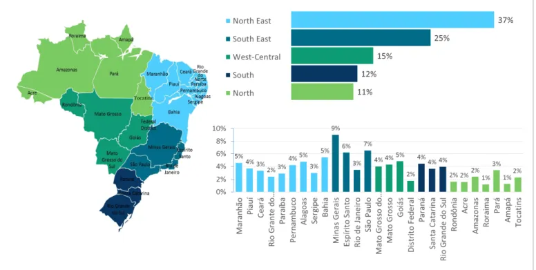
Figure 1 below shows the distribution of respondents by the region, state and type of area.
Brazil, where the population is the densest. In addition, most households interviewed live in
urban areas (77%), and only 23% in rural neighborhoods. Such sample characteristics correspond
closely to population distribution estimations made by the World Bank. (World Bank, 2014)
Figure 1. Location of POF survey respondents. Displayed by region, geographical area (urban or rural), and state. Source: Developed by author, based on data from IBGE Consumer Expenditure Survey 2008-2009
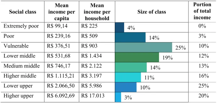
Regarding income of the respondents, most households fell in the vulnerable category,
which consists of families with total monetary income of between R$ 649 and R$ 1,164 per
month. Middle class embodies around 44% of the sample, and around 13% might be regarded as
the Upper class. Mean income data for each social class visualized in Table 1. Such distribution
slightly differs from estimations made by the Brazilian government due to differences in
3%
10%
11%
14%
19%
25%
14%
4%
3% 10% 11% 14% 19% 25% 14% 4% 3% 10% 11% 14% 19% 25% 14% 4%Table 1. Social classes: mean income, size, portion of total income
Social classes: mean income, size, portion of total income
Social class Mean income per capita Mean income per household
Size of class
Portion of total income
Extremely poor R$ 99,14 R$ 225 0%
Poor R$ 239,16 R$ 509 3%
Vulnerable R$ 376,51 R$ 903 10%
Lower middle R$ 531,68 R$ 1.434 12%
Medium middle R$ 746,17 R$ 2.122 13%
Higher middle R$ 1.115,21 R$ 3.197 16%
Lower upper R$ 2.066,50 R$ 5.986 25%
Higher upper R$ 6.092,69 R$ 17.013 20%
Income gap is clearly seen in the Table 1 above: the top earning Higher upper class,
which is only about 3% of the whole population, earns around a fifth of total amount earned in
Brazil; this is more than Extremely poor, Poor and Vulnerable classes together, which represent
almost a half of all Brazilian households.
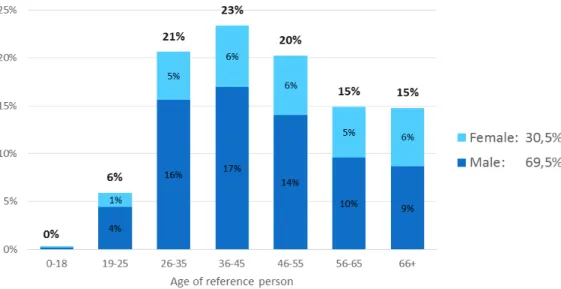
Since gender and age variables are only representing the reference person in the surveying
process – the one that has been interviewed by the IBGE staff – the utility of this demographic
descriptor is limited. Even so, these demographic variables are used in throughout the analysis for
possible insights. In this sample, almost 70% of the reference persons are male. In addition, the
biggest part of respondents are 26 to 55 years old, together making less than two thirds of all
respondents. Reference persons that are older than 56 reach around 30% of all reference people.
Variation is more visible among male respondents, while females make up steadily around 5% to
Figure 2. Respondents by age and gender of the reference person. Source: Developed by author, based on data from IBGE Consumer Expenditure Survey 2008-2009
Consumer Expenditure Survey also provides information about the ownership of credit
cards and health insurance in every household. As seen in Figure 3, only 28,7% off all
households indicated owning a credit card. This figure corresponds to research made by Serviço
de Proteção ao Crédito (SPC), which states that 52 millions of Brazilians use a credit card. ( SPC,
2015)
Even a lower amount of households said they have health insurance. According to
Agência Nacional de Saúde Suplementar (ANS), there are around 42 million people reliant on
health insurance, as of year 2009. (ANS, 2011)
Figure 3. Ownership of credit cards and health insurance. Source: Developed by author, based on data from IBGE Consumer Expenditure Survey 2008-2009
In order to see if there is relationship between ownership of a credit card and health
insurance, Chi-Square test was run. It was discovered that there is indeed a statistically
significant relationship between these two categories (p<0,001). Cramer’s V value is equal to
28.7% 21.7%
71.3% 78.3%
Credit card Health insurance
0,334, which suggests a rather strong association: people that own credit card are more likely to
own health insurance and vice-a-versa.
Regarding living conditions, almost a half of all respondents indicated their living
conditions as good, 40% said that living conditions are just satisfactory, while a tenth of all
households admitted that they have to deal with bad conditions in their domicile.
It can be concluded that the sample of the survey represents the Brazilian population
considerably well in terms of geographical scattering and income distribution. Therefore, the
Consumer Expenditure survey is as a good source of data regarding the whole Brazil: results are
expected to be representative.
5.2.2 General consumption patterns
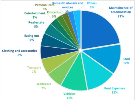
Accumulated annual expenses by Brazilian households in the analyzed categories total to
around R$ 1,581 billion, according to the survey findings. It was discovered that spending is the
highest on accommodation related products and services, totaling around 34% of all the spending
in Brazil, including rent expenses. Distribution of all expenses can be seen in Figure 4.
Figure 4. Composition of total expenses. Source: Developed by author, based on data from IBGE Consumer Expenditure Survey 2008-2009
Alimentation is also a major destination of spending in Brazil: it accounts for around 12%
of the total spending, comparable to spending on vehicles (11%). Transport and healthcare
5.2.2.1 Consumption variations by different social classes
An analysis of total expenses in each expense category by every social class was carried
out to see how spending varies among people having different income. The relationship can be
well seen in a graphic representation of average expenditures by households in each social class
seen in Figure 5 below.
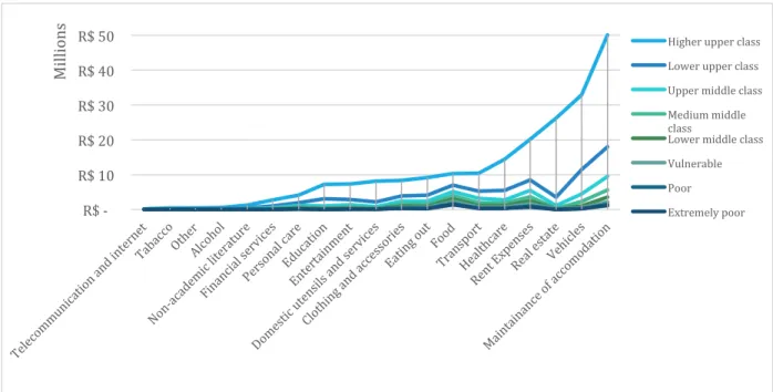
Figure 5. Total expenses by social class. Source: Developed by author, based on data from IBGE Consumer Expenditure Survey 2008-2009
Regardless the expense category, households with higher income spend, according to the
mean values, a higher amount. One-Way Anova test was run in order to test if the differences
between average amounts spent are statistically significant; below, expense categories are
grouped and discussed according to the test results.
In regards to most expense categories, households belonging to Extremely poor, Poor and
Vulnerable classes spend the lowest amounts, which frequently are not statistically different
(p>0,001). Other classes spend different amounts directly proportionate to their income.
In regards to spending on alcohol, statistical significant differences are rare: the only class
that spends an amount that is different from all other classes is the Higher upper class, same
applies to real estate. Similar trend is seen in vehicles category, where only the highest earning
households, namely the Higher middle class and both of the upper classes, spend amounts that are
statistically different from the lower earning classes as well as different among themselves.
R$ - R$ 10 R$ 20 R$ 30 R$ 40 R$ 50
Mi
lli
o
ns Higher upper class
Lower upper class
Upper middle class
Medium middle class
Lower middle class
Vulnerable
Poor
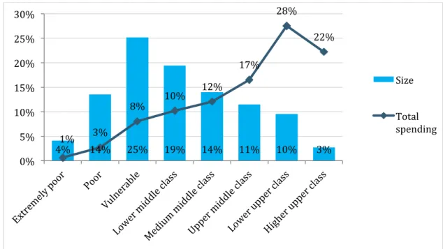
The Figure 6 below demonstrates the proportion of total spending and relative size of each
social class.
Figure 6. Social classes by size and total spending. Source: Developed by author, based on data from IBGE Consumer Expenditure Survey 2008-2009
According to the findings, middle class contributes around 29% of the total consumer
spending, the lower classes make up only 12%, while the upper classes are responsible for half of
the total consumer expenditures. It can be concluded that income gap is a prominent phenomena
in the Brazilian society: a small number of wealthy consumers earn and spend the largest
amounts in the whole economy.
5.2.2.2 Consumption variations by location
As far as geographical distribution is concerned, One-Way Anova tests showed that in all
of the expense categories there are statistically significant differences between regions. The
average spending by regions in all of the analyzed expense categories followed the same pattern:
the smallest expenses were recorded from households living in the North and North East regions
of Brazil, medium were noted in the Central-West, and the highest in South and South-East
regions.
Naturally, it was decided to run a One-Way Anova test to see if there is a relationship
between region and level of income. Statistically significant differences were discovered between 4% 14% 25% 19% 14% 11% 10% 3%
1% 3%
8%
10% 12%
17%
28%
22%
0% 5% 10% 15% 20% 25% 30%
Size
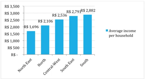
most of the regions. The order is corresponding to the ordering of regions by level of spending,
and visualized in Figure 7.
Figure 7. Regions by average monthly income per household. Source: Developed by author, based on data from IBGE Consumer Expenditure Survey 2008-2009
According to Tukey HSD multiple comparison test, all of the regions are different from
each other except for South East and South regions, which are not statistically significantly
different.
Independent samples T-test was conducted to see how spending varies in relation to the
neighborhood of the household – rural or urban. It was discovered that according to the mean
expenditures, households in urban neighborhoods spend more on all kinds of goods than the ones
in rural regions.
Figure 8. Regions by average monthly income per household. Source: Developed by author, based on data from IBGE Consumer Expenditure Survey 2008-2009
R$ 1,696
R$ 2,106
R$ 2,536 R$ 2,791
R$ 2,882 R$ - R$ 500 R$ 1,000 R$ 1,500 R$ 2,000 R$ 2,500 R$ 3,000 R$ 3,500 Average income per household R$ 2,495 R$ 1,592 R$ - R$ 500 R$ 1,000 R$ 1,500 R$ 2,000 R$ 2,500 R$ 3,000
Urban Rural
However, according to the level of significance, in the some expense categories, namely
food, house maintenance, telecommunications, financial and legal services, real estate and
alcohol, p value was larger than 0,001, meaning that differences are not significant.
Similarly, another Independent Samples T-test was run to see if there significant
differences in levels of income between households living in rural or urban neighborhoods.
Figure 8 illustrates the relationship: in urban neighborhoods, on average, households have a
substantially larger income, which is also statistically significant.
5.2.3 Clustering by absolute values
In order to discover groups of households, which are spending in a similar manner, cluster
analysis was conducted, taking the amounts spent on different goods and services as variables
determining the cluster membership. Two-step clustering technique was chosen due to reasons
explained in the previous section, 4.2 Data analysis.
After numerous experiments with different sets of variables, factors with most complete
data entries (no zero values) were chosen, namely, entertainment, healthcare, clothing and
accessories, personal care, food, and accommodation maintenance expenses.
53% of all households indicated their expenses in the aforementioned expense groups,
therefore were included in the clustering analysis. Initially, two clusters were found to be an
optimal amount, capturing of 47,8% and 52,2% respondents respectively, splitting all households
into a low spending group and a high spending group. Such result brought initial insights: it
suggested that households are different based on overall level of spending rather than preferred
categories. Being so, it was decided to increase the number of clusters in order to explore the data
to a higher extent, and discover whether households might be grouped by other criteria than the
overall expenditure. After multiple experiments, a cluster number of 5 was chosen; this decision
was based on the sizes of clusters, cluster comparison diagrams and Silhouette measure of
cohesion and separation. The chosen solution has a 0,3 value of Silhouette measure of cohesion
and separation, thus the quality of clustering can be considered as fairly good.
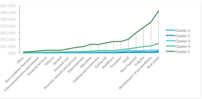
Results of Two-step Cluster analysis with a predetermined amount of 5 clusters brought
similar insights as the aforementioned grouping into 2 clusters. Households were grouped by the
level of spending, rather than destination; Cluster 1 spends the least in all categories, Clusters 2, 3
and 4 spend a medium amount, and Cluster 5 spends the highest amount. Means of expenses and
B2; means of expenditures in each category by each cluster are visualized in Figure 9 below, and
can be found in Appendix B, Table B1. Clearly, the largest differences in spending are seen in the
categories of most expensive goods – vehicles and real estate, as well as accommodation related
expenses.
Figure 9. Means of expenditures by each cluster. Source: Developed by author, based on data from IBGE Consumer Expenditure Survey 2008-2009
Note: The values in R$ are indicated only for visual comparison purposes. These values represent expenses per household, which have bee annualized and expanded in order to create a representative sample.
Chi-Square test and Cramer’s V test analysis were conducted to reveal characteristics of
the five clusters. Tested variables consist of age, race, gender, neighborhood, region, state, level
of education, literacy, social class, ownership of health insurance and credit card, and
employment position. In addition, satisfaction with the living conditions was tested using
One-Way Anova test, as well as age and income.
Gender and type of employment were the only variables in which Chi-square test revealed
no statistically significant difference between clusters. All of the other tested variables proved to
cause statistically significant differences (p < 0,000); results are summarized in the Table 2.
Demographic descriptors of clusters (clustering by absolute amounts)
Demographic descriptors of clusters Cramer’s V test values, included in the table indicate
the perceived strength of association to the descriptive. Estimates used in this thesis for Cramer’s
values and corresponding strength of association can be found in the Appendix A, Table A1.
R$0 R$1,000 R$2,000 R$3,000 R$4,000 R$5,000 R$6,000 R$7,000
Demographic descriptors of clusters (clustering by absolute amounts)
Mean values
Cramer’s V Cluster 1 Cluster 2 Cluster 3 Cluster 4 Cluster 5 Comments
Size 15,4% 29,4% 27,5% 20,2% 7,5%
0,280 Social class / Income per household Poor to Lower middle class Mean: 1310 R$ Vulnerable to Medium middle class Mean: 2002 R$ Vulnerable to Higher middle class Mean: 2582 R$ Lower middle class to Lower upper class Mean: 4260 R$
Higher middle class to Higher upper class Mean: 7674 R$
Indicated classes make up at least 60% of the population
0,064 Age of ref. person 26-45 Mean: 43,75 26-45 Mean: 45,32 36-55 Mean: 46,46 36-55 Mean: 46,45 36-55 Mean: 48,74
2 largest age groups. 3 and 4- not significantly different 0,122 Race of ref.
person
Pardo 60,2% 54,9% 45,6% 35,4% 22,3% Percentage of
Yellow and Indigenous are below 1%
White 29,9% 35,8% 44,7% 56,3% 71,5%
Black 8,7% 8,4% 8,7% 7,3% 5,0%
0,238 Neighborhood Urban 65,8% 78,6% 83,7% 92,0% 97,6%
Rural 34,2% 21,4% 28,0% 8,0% 2,4%
0,215 Region § North
§ North East
§ North East § Central West
§ North East § South East
§ South East § South
§ South East Regions with highest % in cluster 0,193 Education of
ref. person
Primary 29,3% 26,3% 25,9% 19,2% 14,7% Highest
achieved education
Secondary 68,0% 65,7% 63,9% 60,6% 49,3%
Higher 2,7% 7,4% 10,3% 20,2% 36,0%
0,184 Literate portion of people 78,7% 85,8% 89,2% 95,4% 98,5%
Satisfaction with living conditions (mean)
2,29 2,38 2,42 2,53 2,66 1-Bad
2-Satisfactory 3-Good 0,236 Ownership of: Credit card 20,8% 29,9% 35,5% 48,3% 62,0%
0,328 Health
insurance
10,4% 19,0% 26,9% 43,4% 64,0%
0,171 Type of accommodation
House 96,6% 95,1% 93,3% 85,4% 73,6%
Flat 2,4% 4,4% 6,2% 18,9% 26,3%
As can be expected, clusters are significantly different by their income, ranging from low income Cluster 1 to the high earning Cluster 5. This association was found to be among the strongest ones, as seen by the Cramer’s V value of 0,280. To further explore the differences, One-way Anova test was conducted, including all of the expense groups and the cluster membership variable. The test showed statistically significant differences among spending in all expense categories, amount directly proportional to the Cluster number. According to Tukey HSD post-hoc tests, the only similar clusters are Cluster 1 and Cluster 2, with no statistically significant differences among some of the expense groups, including telecommunications, real estate and vehicles. Table showing the means for each cluster can be found in Appendix B, Table B1.
Regarding the dominating race within each cluster, Cluster 1 and Cluster 2 consist mostly of people who identified themselves as being Pardo1. Cluster 3 contains both white and Pardo in equal proportions, while Cluster 4 and Cluster 5 are dominated by white Brazilians. Proportion of Black people does not vary much within Clusters 1 to 4, though decreases to 5% in Cluster 5. Amount of people that identified themselves as being Indigenous or Yellow is negligible, containing less than 1% in each cluster.
As far as location of households is concerned, the highest portion of people living in rural areas belongs to Cluster 1, being a third of the whole cluster. This amount gradually decreases when moving towards Cluster 5, where rural neighborhoods are home to only a negligible amount of respondents. In addition, there are statistically significant differences between regions. Cluster 1 and Cluster 2 mostly settle in the North East, 49,2% and 45,9% of the cluster members respectively. Majority of Cluster 3 is scattered in the North East (35,9%) and South East (22,2%). Members of Cluster 4 are found mostly in South East, North and South. The absolute majority of Cluster 5 lives in the South East (64,3%).
In addition, there is a clear distinction in education between clusters. Highest educated people belong to Cluster 5, with the highest proportion of persons having a university degree or equivalent. The percentage of such people drastically drops when moving toward Cluster 1; the latter holds the biggest portion of people with just primary education or simple literacy courses among all of the clusters.
1
As far as literacy within clusters is concerned, highest proportion of people with reading and writing abilities are in Cluster 5, almost 99%. Literacy drops gradually when moving towards Cluster 1, where illiteracy is as high as 21,3%.
One-Way Anova revealed that Cluster 1 is the least content with the living conditions, while Cluster 5 is the most content; Tukey HSD test showed that differences between clusters in this dimension are highly significant.
Regarding ownership of a credit card and health insurance, results are in alignment with the analysis: smallest portions of owners belong to Cluster 1, while the largest to Cluster 5. Interestingly, ownership of health insurance was discovered to be the factor with the strongest association, as indicated by Cramer’s V test value of 0,328.
Type of accommodation varies among clusters. Most households in every cluster live in houses: in total, 91,3% of the total amount of analyzed households. Interestingly, the biggest portion of apartments is observed within Cluster 5.
In conclusion, based on expenses on food, accommodation maintenance, healthcare, clothing and accessories, entertainment and personal care, Brazilian consumers could be divided into 5 clusters.
Cluster 1 mostly consists of consumers with the lowest household income nationwide, living in Northern parts of Brazil; a third has settled in rural neighborhoods. Cluster members are predominately Pardo race, have achieved the lowest levels of education and exhibit the lowest satisfaction with their living conditions in the country. Mostly living in private houses, with very low percentage of people owning health insurance and credit cards, these consumers spend the least money in all expense groups among the clusters. Cluster 2, Cluster 3 and Cluster 4
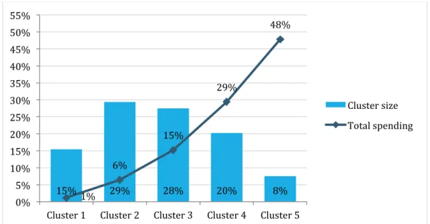
In Figure 10, clusters are presented by their proportionate size and spending, further
strengthening illustrating that Cluster 5 spends extremely higher amounts – around 48% of all
consumer spending emerges from only 8% of the households. These results are analogous to
output generated by assessing the social classes, visualized in Figure 6 in the previous section.
Figure 10. Clusters by size and total spending (clustering by absolute amounts). Source: Developed by author, based on data from IBGE Consumer Expenditure Survey 2008-2009
Such results to clustering are not surprising: people with higher levels of education have
higher income, better access to health insurance and larger need for credit cards; therefore,
disposable income allows them to spend more on all kinds of goods and services in terms of
quantity or quality.
5.2.4 Clustering by percentile amount
The absolute amount spent on the analyzed kinds of goods and services is immensely
related to income size, as discovered in the previous section. That being so, it is worth examining
the consumer spending in Brazil from another perspective: based on distribution of their
expenses. The following question is expected to be answered: which households choose to spend
a similar portion of their resources to the same types of goods and services, and do these groups
share similar demographic criteria? To explore such considerations, absolute values in each
category of expenses were transformed to percentile values for every household, and used for the
cluster analysis.
15% 29% 28% 20% 8%
1% 6% 15% 29% 48% 0% 5% 10% 15% 20% 25% 30% 35% 40% 45% 50% 55%
Cluster 1 Cluster 2 Cluster 3 Cluster 4 Cluster 5
Cluster size
All 20 expense groups were used for clustering. A total 49,526 cases were included in the
analysis; 6,063 were excluded due to missing values 2. Two step clustering method was applied,
and, after multiple tests regarding the amount of desired clusters, five clusters was estimated to be
an optimal number. Silhouette measure of cohesion and separation was estimated as 0,1, which is
relatively low; however, experimenting with desired amount of clusters and types of variables
included in the analysis did not lead to any higher quality solution. All of the variables were
equally important predictors of cluster membership in the Two-step Clustering process.
In the Table 3 below, means for each cluster are presented. Values are formatted in the
way that red represents the lowest average percentage among all clusters devoted to a particular
expense category, white shows medium values, while blue – the highest average percentage.
Cluster means and standard deviation, centroids and full clusterwise importance tables for each
factor, can be found in Appendix B, Tables B3 and B4.
2
Zeros as missing values were declared only for Food and Maintenance categories. In other cases, 0 is
Table 3. Means of percentile expenditures in every category, by clusters
Means of percentile expenditures in every category, by clusters
Expense category
Mean of Expenditures (%)
Cluster 1 Cluster 2 Cluster 3 Cluster 4 Cluster 5
Literature 0,39 0,55 0,57 * 1,73 0,34
Domestic 1,31 * 4,76 1,23 * 0,96 * 0,73 Clothing 5,15 5,48 * 10,17 * 6,51 * 4,77
Vehicles * 27,06 3,88 3,44 2,38 1,98
Telecommunications 0,17 0,13 0,24 * 2,09 0,11 Transport * 5,63 * 4,9 * 10,67 * 6,40 * 3,68 Eating Out 3,27 3,4 * 9,67 * 5,50 * 2,22
Tobacco 0,29 0,31 0,46 * 3,64 0,42
Alcohol 0,17 0,15 0,11 * 1,93 0,09
Other 0,11 0,12 * 0,44 0,11 0,05
Financial * 3,17 * 10,17 2,06 1,84 1,49
Real Estate * 5,74 0,32 0,14 0,14 0,1
Education * 1,17 * 4,92 0,75 0,59 * 0,31 Rent * 9,06 13,22 12,81 * 15,04 * 21,02 Entertainment 2,38 2,67 * 4,61 2,62 * 1,5 Travelling * 4,87 * 1,29 1,05 0,87 * 0,58 Personal Care 2,08 * 2,64 * 5,27 * 3,23 1,93 Healthcare 4,56 * 12,15 4,69 4,93 * 5,98 Food * 11,26 * 13,44 * 16,03 * 21,6 * 27,82 Maintenance House * 12,17 15,48 15,58 * 17,87 * 24,89
One-way Anova test was run to see if means of average expenditures are different up to a
statistically significant level. It was discovered that in each category there is at least one cluster
that is different from every other cluster; such means are marked with an asterisk symbol in the
Table 3 above. The only category where all the clusters are statistically significantly different
from each other is food: Cluster 1 spends the least percentage amount, then sequentially Cluster
2, Cluster 3, Cluster 4 and finally, the largest portion is spent by Cluster 5.
This analysis brought interesting results. Cluster 1 notably spends larger percentile
amounts on vehicles, travelling and real estate than any other cluster, while expenses such as food
and house maintenance expenses are comparably the least notable, in terms of percentage of all
expenses. Cluster 2 can be distinguished by its large spending on healthcare, education and
financial and legal services. For Cluster 3, personal care, clothing, eating outside the house and