For citation: Ekonomika regiona [Economy of Region]. — 2016. — Vol. 12, Issue 2. — pp. 560-568 doi 10.17059/2016–2–20
UDC: 330.564
J. R. Alm a), R. A. Grigoryev b), M. V. Kramin b), T. V. Kramin b) a) Tulane University (New Orleans, USA) b) Kazan Innovative University named ater V. G. Timiryasov (Kazan, Russian Federation; e-mail: [email protected])
TeSTing kuzneTS’ hypoTheSiS for ruSSian regionS:
TrendS and inTerpreTaTionS
1The paper established a number of "stylized facts", one of which is a conirmation of the S. Kuznets’ hy -pothesis of the nonlinear dependence between the degree of inequality in income distribution and welfare economic systems on the example of a group of Russian regions for the period 2002–2012. It is shown that, for a given sample, the welfare and economic growth factors amplify their inluence on inequality in income distribution in the post-crisis period. The monotonous growth of income inequality which was observed be -fore the crisis of 2008 is slowing in the process of raising the per capita gross regional product (GRP) dur-ing the post-crisis period, and for the foreseeable future, in some regions, its direction can be reversed, while maintaining a trend of socio-economic development. Despite the persistence over time of a convex nature of S. Kuznets’ curve for Russian regional data, its parameters changed during the reporting 2002–2012 period. The maximum point of the curve shifts to the left, its convexity increases. These facts indicate that the income inequality growth of the Russian regions’ as a result of growth of per capita GRP is slowing. For some regions in the post-crisis period, the income inequality does not grow with the growth of per capita GRP, or it even re -duces. This fact can be attributed to the implementation of the Russian federal socially oriented projects and programs in recent years. The results can be used for the development of regional economic policy in order to regulate the level of income distribution inequality in the regions of Russia.
Keywords: inequality of income distribution, economic growth, Gini coeicient, competitiveness of regions, re-gression modeling, gross regional product, income, post-crisis period, regional policy, poverty reduction
1
1. Introduction
Inequality of income distribution over time has recently returned to prominence in economic de
-velopment. A number of scientists have directly linked income inequality and economic growth, see, for example, Barro [1, 2]. This paper conirms several hypotheses related to income inequality. In particular, the Kuznets’ hypothesis [3] about the nonlinear dependence between the level of in
-equality and wealth in economic systems is veri
-ied using the data of 79 Russian regions for the period 2002–2012.
In present work, the assumption of homogene
-ity of the mechanism of mutual inluence of in
-come inequality and economic development in the Russian regions is done and veriied. This assump
-tion allows considering a relatively short time pe
-riods in the simulation in the presence of a large sample of spatial observations. Initially, we keep the main explanatory variable and the mecha
-nism of constructing a model in accordance with the original formal characteristics of the Kuznets’
1 © Alm J. R., Grigoryev R. A., Kramin M. V., Kramin T. V. Text. 2016.
model, but we modiied the object of study and a combination of factors that affect income inequal
-ity in the regions of Russia.
Getting a stable, well-speciied econometric model of the Kuznets’ curve permits to predict soundly the level and dynamics of income ine
-quality in the Russian regions, depending on their level of wealth. The aim of this study is not the at
-tempt to verify the effect of the level of income in
-equality separate, very important factors, such as migration, employment and so forth. This is a sub
-ject for future research.
2. Literature review
In 1955, based on the analysis of empirical data of the major developed countries in the nine
-teenth century and the irst half of the twentieth century, Kuznets [3] suggested a speciic nonlin
-ear dynamic process relating the level of inequal
sectors (labeled A and B, respectively), which dif
-fered by the level and structure of income. He hy
-pothesized that economic development occurred with the non-agricultural sector expanding and agricultural sector narrowing. On the basis of ab
-stract data, Kuznets then traced the change in in
-equality in population incomes when the agricul
-tural sector (A) share of total output changed from 0.8 to 0.2. To assess the impact of various struc
-tural parameters on the shape of the curve charac
-terizing the dynamics of inequality, Kuznets con
-sidered several models with different values of key parameters. As a result, he was able to demon
-strate that changes in its parameters affected the shape of the income distribution curve (in particu
-lar, its maximum point) but not its general charac
-ter (or the inverted U curve).
The simulation results obtained by Kuznets have a simple mathematical interpretation. The test indicator (in this case, the level of income inequality), is affected by several (two or more) factors: an increase in some factors reduces this level and an increase in the others increases it. Additionally, the effect of the former (latter) fac
-tors increased (reduced) over time due to the structural changes in the economic system. The maximum point of the curve describes a struc
-ture of the economic system in which the total effect of the factors that increase inequality be
-comes weaker than the overall impact of the other factors.
A mathematical formalization of the process described in Kuznets [3] is provided in the Anand and Kanbur study [4, 5]. Their model highlights the structural components of the overall level of inequality, an in-sector component (a monotoni
-cally increasing curve), and a trans-sector compo
-nent (inverted U-shaped curve).
All of the above leads to a number of prelimi
-nary conclusions:
1. Kuznets’ hypothesis is based on the assump
-tion and ra-tionale of the impact of structural re
-forms and the development of economic systems on the level of inequality in income distribution.
2. A non-linear character of the curve of the dynamics of inequality (inverted “U” curve) is de
-termined by the changes of various factors in the process of structural transformation. The shape of the curve can also change over time.
3. Kuznets’ hypothesis has been conirmed for any economic system (country, region), the group of economic systems, in any period of time, during which there are structural transformations.
The Kuznets’ work provides a basis for the analysis of the nonlinear dependence of the in
-come inequality and the welfare on the economic
system. However, there is no econometric mode
-ling based on these results in the aforementioned Kuznets' paper.
2.1. Econometric modeling for Kuznets’ hy-pothesis testing
Ahluwalia [6, 7] was among the irst to test Kuznets’ hypothesis econometrically. He used the share of income of all groups in the country dis
-tributed by income quintiles as indicators of in
-come inequality (or the same indicators as in Kuznets [3]). The log of per capita GDP was used to indicate the level of welfare of the country. Some other work testing Kuznets’ hypothesis do not use the share of income of certain groups of the pop
-ulation as the dependent variable, instead using the Gini coeficient [8, 9] as the measure of ine
-quality of income distribution; see, for example, Papanek and Kyn [10] and Huang [11]. Other alter
-native measurements of inequality are also known [12, 13].
In general, these works can be divided into two groups: ones that follow Ahluwalia [10, 11] and use the logarithm of per capita GDP as an inde
-pendent variable in their models [10]), and others who did not [11]). Despite the similarity of the two approaches, their respective mathematical models and the corresponding interpretations are quite different.
2.2. Regional aspect and Russian domestic studies
Most of the works of the early period were de
-voted to deining the relationship between income distribution and economic growth using data from the countries [4, 5, 6, 7, 10, 14, 15]. In recent years, income distribution on economic growth in de
-veloping countries [16] is under the focus of the evaluation.
It is obvious that the country context is still causing a lot of criticism regarding signiicant dif
-ferences in the process of income data collection [17, p. 26, 18, p. 196], as well as because of the ina
-bility to identify the speciics of each country [19, p. 60]. The necessity of the regional analysis is re
-lected in the work by M. Partridge [20, p. 1021], which states that the distribution of income is originally different for each country of the World.
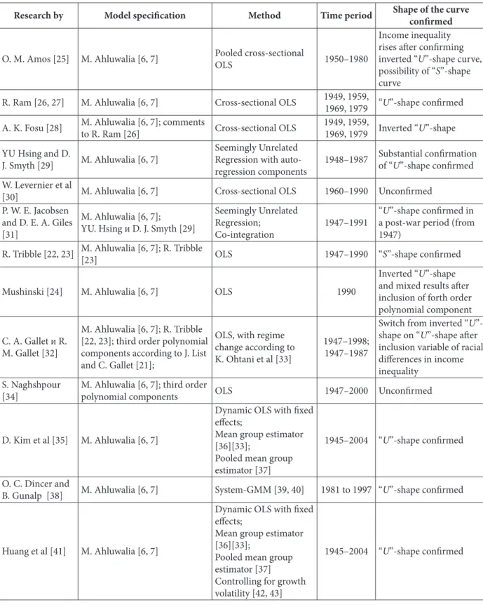
Table 1 shows the results of Kuznets’ hypothe
-sis testing based on US regional data. It should be noted that most studies, presented in Table 1, pri
-marily use panel data.
It is noted also that results greatly vary, due to the use of different time periods, different mod
-els speciication, by integrating the third order component [21–23] and fourth order component [24] in the original speciication.
Several papers devoted to the testing and as
-sessment opportunities for the application of the Kuznets’ hypothesis for Russian regional data have been made in recent years by Russian scien
-tists. A brief review of them is submitted in the ar
-ticle by Ratnikova and Furmanov [44].
From an econometric point of view, one should mention the Demidova’s indings [45], in which the Kuznets’ hypothesis received conirmation on panel data for 84 regions of Russia during the pe
-riod 2001–2006. The funds coeficient is used as a
Table 1
Kuznets hypothesis testing on US regional data
Research by Model speciication Method Time period Shape of the curve conirmed
O. M. Amos [25] M. Ahluwalia [6, 7] Pooled cross-sectional
OLS 1950–1980
Income inequality rises ater conirming
inverted “U”-shape curve,
possibility of “S”-shape curve
R. Ram [26, 27] M. Ahluwalia [6, 7] Cross-sectional OLS 1949, 1959,
1969, 1979 “U”-shape conirmed
A. K. Fosu [28] M. Ahluwalia [6, 7]; comments
to R. Ram [26] Cross-sectional OLS
1949, 1959,
1969, 1979 Inverted “U”-shape
YU Hsing and D.
J. Smyth [29] M. Ahluwalia [6, 7]
Seemingly Unrelated Regression with auto-regression components
1948–1987 Substantial conirmation
of “U”-shape conirmed
W. Levernier et al
[30] M. Ahluwalia [6, 7] Cross-sectional OLS 1960–1990 Unconirmed
P. W. E. Jacobsen and D. E. A. Giles [31]
M. Ahluwalia [6, 7]; YU. Hsing и D. J. Smyth [29]
Seemingly Unrelated Regression;
Co-integration
1947–1991
“U”-shape conirmed in
a post-war period (from 1947)
R. Tribble [22, 23] M. Ahluwalia [6, 7]; R. Tribble
[23] OLS 1947–1990 “S”-shape conirmed
Mushinski [24] M. Ahluwalia [6, 7] OLS 1990
Inverted “U”-shape
and mixed results ater inclusion of forth order polynomial component
C. A. Gallet и R. M. Gallet [32]
M. Ahluwalia [6, 7]; R. Tribble [22, 23]; third order polynomial components according to J. List and C. Gallet [21];
OLS, with regime change according to K. Ohtani et al [33]
1947–1998; 1947–1987
Switch from inverted “U
”-shape on “U”-shape ater
inclusion variable of racial diferences in income inequality
S. Naghshpour [34]
M. Ahluwalia [6, 7]; third order
polynomial components OLS 1947–2000 Unconirmed
D. Kim et al [35] M. Ahluwalia [6, 7]
Dynamic OLS with ixed efects;
Mean group estimator [36][33];
Pooled mean group estimator [37]
1945–2004 “U”-shape conirmed
O. C. Dincer and
B. Gunalp [38] M. Ahluwalia [6, 7] System-GMM [39, 40] 1981 to 1997 “U”-shape conirmed
Huang et al [41] M. Ahluwalia [6, 7]
Dynamic OLS with ixed efects;
Mean group estimator [36][33];
Pooled mean group estimator [37]
Controlling for growth volatility [42, 43]
dependent variable characterizing the level of in
-equality, and she considered the real average in
-come per capita as the major independent varia
-ble. Ratnikova and Fourmanov, referring to the re
-sults obtained by Demidova, pay attention to the instability of the model constructed by Demidova; that is, the regression results are signiicantly modiied by the exclusion of Moscow city data of the number of observations of the model.
The analysis of the current economic and de
-mographic situation using the structural decom
-position of inequality into normal and redundant components is performed by A. Y. Shevyakova, A. J. Kiruta [46]. Their indings contradict the cur
-rent view of the inequality as an inevitable but temporary side effect of economic growth.
The authors argue that economic growth favors the growth of a normal inequality 1, whereas exces
-sive inequality generated by numerous factors, in
-cluding institutional, does not decrease during the period of economic growth and needs the long-term and various adjustments. In particular, the A. Y. Sheviakov and A. J. Kiruta showed that the canonical Kuznets’ hypothesis, estimated for the Russian regions, is not conirmed. However, it be
-comes correct with a high degree of statistical sig
-niicance, if the index of overall inequality would be replaced with the index of normal inequality in it.
Moreover, a number of macroeconomic indi
-cators are positively correlated with normal ine
-quality and negatively correlated with the exces
-sive one. Such an effect is, as noted by the authors, can not be detected using traditional indicator of overall inequality. In addition, the authors found that the most powerful factor in explaining mac
-roeconomic differences between the regions of Russia was the difference between normal and ex
-cessive inequality levels.
An important achievement of A. Y. Novikov and A. J. Kiruta is also a study of the effect of income inequality on migration in the Russian regions.
M. Y. Malkina conirmed the existence of the negative effect of the level of economic develop
-ment on the uniformity of income in regions of the Russian Federation at the present stage (due to the fact that most of them are found on the up
-stream stage of the Kuznets’ curve) [47]. In addi
-tion, the review of the works of Russian scientists presented the M. Y. Malkina is also noteworthy.
In the paper by I. P. Glazyrina and I. A. Klevakina [48], it was also concluded that for the majority of regions the real GDP per capita increase cor
-1 Please refer to description of notion on normal inequality [46, p. 5, 23].
responds to the Gini coeficient rising, that is, they are on the ascending branch of the Kuznets’ curve, and only Moscow and Khanty-Mansiysky Autonomus District 2 have overcome the peak of the Kuznets curve and passed on the descending branch of the curve [48, p. 117–121].
G. P. Litvintseva, O. V. Voronkova and E. A. Stu- kalenko [12] proposed and tested approach to benchmarking regional incomes based on the rel
-ative cost of a ixed basket of goods and services in the region to the cost of the same set in the Russian Federation.
In the same paper, the calculation of Gini co
-eficients taking into account social transfers in kind for groups of regions was made. The authors concluded that this reinement decreased interre
-gional differentiation in Russia.
On the basis of summarizing the results of pre
-vious publications tested the Kuznets’ hypothesis, in current work, we tested it for Russian regional data for the 2002–2012 period.
3. Speciication
We estimate the following equations [10, 11]:
(
)
(
)
2log (log ) ,
Gini= α + β PCG + g PCG + δ + εD (1)
2
,
Gini= α + βPCG+gPCG + δ + εD (2) where Gini is the annual regional Gini coeficient; PCG is per capita gross regional product adjusted for annual price indexes (“top wave” variable se
-lection refers to the division of this variable on 1 000 000 for illustrative purposes of simulation results); D is a vector of dummy variables (not included when both space and time ixed effects are used at the same time); and α, β, g, δ (vector) and ε are coeficients and the error of the regres
-sion, respectively. We chose such stochastic equa
-tions based on the fact that they are most common in the economic literature for testing Kuznets’ hypothesis.
4. Data description
We use the data of Federal State Statistics Service of Russian Federation (Rosstat). The fol
-lowing variables are used:
— PCG denotes the gross regional product per capita, adjusted for the annual price index. GRP per capita data were obtained from on the oficial website of Rosstat 3 in the national accounts sec
-2 Khanty-Mansiysk autonomous district is the subject of Russian Federation, but oicially and in this study is accounted as a part of the Tyumen Oblast.
tion. Price index 1 was used as a delator to adjust the GRP obtained from "Regions of Russia. Socio-Economic Indicators" periodicals located on the same site;
— Gini denotes Gini coeficient 2 taken as an in -dicator of differentiation of income distribution in the region. This ratio was also obtained from "Regions of Russia. Socio-Economic Indicators." It is worth noting that the Gini index for 2001 is not available for the year 2002, which means that we cannot do a full comparison of our results with the models of Demidova [45] and Ratnikova and Fourmanov [44]. The use of composite data from other sources indicates a substantial difference in the method of calculation and, as a consequence,
1 We assume that the use of adjustments for price index (Consumer Price Index) is appropriate as a substitute for the GDP delator for the transformation of nominal GDP to real. 2 he method of calculating the Gini coeicient is ixed in Goskomstat Regulation (Decree of State Statistical Committee of Russian Federation 16.07.1996 № 61 “On approving the methods of calculating the monetary income and expenses of the population and the main social-economic indicators of the living standard).
the deterioration of the simulation results. In ad
-dition, we follow the classical works testing the Kuznets’ hypothesis [6, 7, 10, 11].
We work with panel data including all regions of Russia, except for the Chechen Republic, as well as regions that were included in the larger subjects of Russian Federation in the process of creating larger regions. The number of regions in the sam
-ple after this adjustment was 79. Regression mod
-eling covers the period between 2002 and 2012.
5. Regression and simulation results
We irst estimate Kuznets’ hypothesis using equation (1). The regression results are presented in Table 2.
Anticipating the analysis of simulation results, it should be noted that a relatively short time pe
-riod does not create econometric problems in panel data regression analysis due to the large number of spatial observations in the panel. In ad
-dition, a large number of observations of the panel also allows observing Kuznets’ curve in the rela
-tively short periods due to the fact that Russian regional data are much more homogeneous than
Table 2
Regression results using equation (1)
Model number Dependent variable: Gini — Regional Gini coeicient
1 2 3 4 5 6 7 8
Beginning of the period 2002 2002 2002 2002 2002 2002 2009 2009
End of the period 2006 2006 2006 2012 2012 2012 2012 2012
Cross-section ixed efects No No Yes Yes Yes Yes Yes Yes
Period ixed efects No No No No Yes No No No
С 1.3068
(0)
0.1337 (0.6140)
–0.2008 (0.1773)
–0.4205 (0)
–0.3708 (0)
–0.3682 (0)
–0.9445 (0)
–0,9083 (0)
Log (PCG) –0.2056
(0)
0.0159 (0.7416)
0.0793 (0.0034)
0.1149 (0)
0.1036 (0)
0.1049 (0)
0,2113 (0)
0,2154 (0)
(Log (PCG))2 0.0109
(0)
0.0004 (0.8438)
–0.0025 (0.0388)
–0.0039 (0)
–0.0033 (0)
–0.0034 (0)
–0,0083 (0)
–0,0089 (0)
d (Moscow) 0.1876
(0)
d (Tyumen) 0,0385
(0.0072)
d_2008 0,0047
(0,0005)
d_2011 –0,0059
(0.0001)
d_2012 0,0065
(0)
R-squared 0.3953 0.6348 0.9536 0.9093 0.9182 0.9131 0.9698 0,9762
Prob(F-statistic) 0 0 0 0 0 0 0 0
the data of different countries, which are consid
-ered in the classical Kuznets model.
Therefore, we made the assumption of homo
-geneity of the mechanism of mutual inluence of income inequality and economic development in the Russian regions, similarly to Partridge’s pa
-per [20, p. 1021], who analyzed states of the USA. Thus, the present study largely follows the orig
-inal Kuznets model: explained variable of the model and the mechanism of model building are preserved. However, the object of study and a set of factors to be included in the model are modiied.
In Model 1 we do not use ixed effects, and the estimation is for the period 2002–2006. It can be characterized by a relatively low degree of ex
-plaining the difference of the dependent variable (39.5 %) and instability. In Model 2, several dummy variables are added (d(Moscow), d(Tyumen)). This speciication led to the outcome where the coefi
-cients at all the key explanatory variables became insigniicant (see Model 2).
This fact, to a certain extent, is in agree
-ment with the result obtained by Ratnikova and Furmanov [44]. However, when using the method of least squares for panel data with spatial ixed effects (Model 3), the speciication improves, and the results conirm the Kuznets’ hypothesis.
Further expansion of the data for the period 2002–2012 also improves the model speciication and its stability signiicantly for all types of ixed effects used (Models 4, 5, 6). The Kuznets’ hypoth
-esis is fully conirmed for these speciications. Also, using temporary dummy variables allows us to track the impact of the crisis on the relation
-ship (Model 6).
Table 1 clearly manifests the inluence of the crisis of 2008: the sign of the coeficient at the
dummy variable d_2008 is positive and statisti
-cally signiicant, whereas for other periods (2002, 2004–2006, 2011) the sign of the relevant coefi
-cient is negative. All aforementioned dummies are highly signiicant; the signiicance of dummy var
-iables for 2002, 2004–2006 is shown in the mod
-eling results presented in Table 3. The crisis of 2008 gives a small but pronounced effect on the stochastic equation describing the Kuznets’ curve for Russian regional data.
Models 7 and 8 in Table 2 are built on a sam
-ple of post-crisis period of 2009–2012. Along with the stability of these models we again observe the conirmation of the Kuznets’ hypothesis. However, the form of stochastic dependence is different from the form generated by the sample 2002–2012 period (Models 4–6 in Table 1) and for the sample 2002–2006 (Model 1–3 in Table 2).
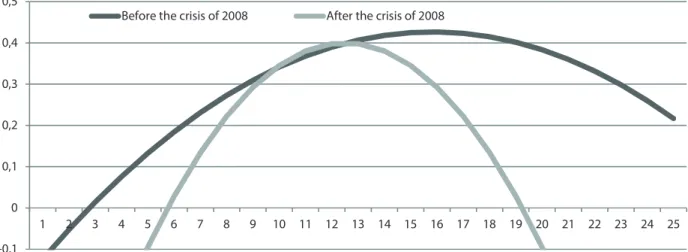
In order to study the dynamics of changes in the shape of the Kuznets’ curve for Russian re
-gions in the 21st century, we construct such curves on panels 2002–2006 (or before the crisis, using Model 3 of Table 2) and for the period of 2009– 2012 (or after the crisis, using Model 7 of Table 2). See Figure 1.
According to Figure 1, it can be seen that as the maximum point of the curve shifts to the left (turning point), the curve becomes less lat (more concave). It is important to note that the value of the variable Log (PCG) for Russian regions (or the variable that is an argument for the constructed curves in Figure 1) varies in the interval 9;13 in a given time period.
Figure 1 suggests the following conclusions: 1. There is an increase in the inluence factors of welfare and economic growth on inequality in
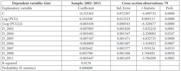
Table 3
Regression results extending Model 6 of Table 2
Dependent variable: Gini Sample: 2002–2012 Cross section observations: 79
Explanatory variable Coeicient Std. Error t-Statistic Prob.
C –0.325362 0.072307 –4.499732 0.0000
Log (PCG) 0.101048 0.012523 8.069113 0.0000
(Log (PCG))2 –0.003436 0.000543 –6.328477 0.0000
D_2002 –0.007005 0.001828 –3.832210 0.0001
D_2004 –0.003482 0.001547 –2.250003 0.0247
D_2005 –0.007107 0.001471 –4.832735 0.0000
D_2006 –0.004809 0.001407 –3.418923 0.0007
D_2007 0.002642 0.001377 1.919124 0.0553
D_2008 0.003788 0.001368 2.768492 0.0058
D_2011 –0.005447 0.001439 –3.784209 0.0002
R-squared 0.9178
Probability (F-statistic) 0.000000
income distribution in the post-crisis period in Russia.
2. In the post-crisis period, the trend in the monotonous growth of income inequality in the process of raising the per capita GRP is slowing, and in the foreseeable future, its direction can be reversed, at least for some Russian regions, while maintaining a trend of socio-economic development.
If instead we use equation (2), the Kuznets’ hypothesis for the period 2002–2012 is also con
-irmed. See Table 4.
It should be noted that the model presented in Table 4 is constructed by using both spatial and temporal ixed effects.
6. Conclusion
Our main result is a conirmation of the Kuznets’ hypothesis for Russian regions in the pe
-riod 2002–2012. In addition, we ind strong sup
-port for the Kuznets’ hypothesis for several peri
-ods of time (e.g., before the crisis of 2008 and in the post-crisis period), and also for different ex
-planatory variables (e.g., with the logarithm of per capita gross regional product and without it).
Despite the persistence over time of the con
-cave nature of the Kuznets’ curve for Russian re
-gional data, its parameters apparently changed during the 2002–2012 years. Over time, we ind that the maximum point of the curve has shifted to the left, and its concavity has increased. These results indicate, that the growth of inequality in income distribution in the Russian regions by GRP per capita growth is getting slower. For some Russian regions in the post-crisis period, income inequality does not seem to grow with the growth of GRP, and in fact, inequality tends to fall, perhaps because of the implementation of the Russian federal socially oriented projects and programs in Russia in recent years. These re
-sults also indicate the possible impact of factors affecting the level of differentiation of income in the region, indicating either that an acceleration of structural reforms in the Russian economy in the post-crisis period is taking place, or that the impact of factors driving income inequality has changed over recent time.
One of the areas of future research will be de
-veloping a generalized Kuznets’ model, in order to test the feasibility of introducing additional fac
-tors, which may have potentially signiicant im
-pact on the level of income differentiation (such as labor migration lows, unemployment, etc.). -0,1
0 0,1 0,2 0,3 0,4 0,5
1 2 3 4 5 6 7 8 9 10 11 12 13 14 15 16 17 18 19 20 21 22 23 24 25 Before the crisis of 2008 After the crisis of 2008
Note: The ordinate of the graph corresponds to the Gini coeicient, where the abscissa is Log (PCG). Fig. 1. Comparing the Kuznets’ curve for Russian regions before and after the crisis
Table 4
Regression results using equation (2)
Dependent variable: Gini Sample: 2002–2012 Cross section observations: 79 Explanatory variable Coeicient Std. Error t-Statistic Prob.
C 0.380432 0.002065 184.1864 0.0000
PCG/1000000 0.001963 0.017477 0.112294 0.9106
(PCG/1000000)2 –0.031240 0.012672 –2.465358 0.0139
R-squared 0.914291
Probability (F-statistic) 0.000001
References
1. Barro, R. J. (2000). Inequality and Growth in a Panel of Countries. Journal of Economic Growth, 5(1), 5–32.
2. Barro, R. J. (1996). Determinants of Economic Growth: A Cross-Country Empirical Study (No. w5698). National Bureau
of Economic Research, 118.
3. Kuznets, S. (1955). Economic Growth and Income Inequality. he American Economic Review, 45(1), 1–28.
4. Anand, S. & Kanbur, S. R. (1993). he Kuznets Process and the Inequality —Development Relationship. Journal of
Development Economics, 40(1), 25–52.
5. Anand, S. & Kanbur, S. R. (1993). Inequality and Development. A critique. Journal of Development Economics, 41(1),
19–43.
6. Ahluwalia, M. S. (1976). Inequality, Poverty and Development. Journal of Development Economics, 3(4), 307–342.
7. Ahluwalia, M. S. (1976). Income Distribution and Development: Some Stylized Facts. he American Economic Review,
128–135.
8. Ceriani, L. & Verme, P. (2012). he Origins of the Gini Index: Extracts from Variabilità e Mutabilità (1912) by Corrado
Gini. he Journal of Economic Inequality, 10(3), 421–443.
9. Gini, C. (1912). Variabilita e Mutabilita, Contributo Allo Studio Delle Distribuzioni: Relazione Statische. Studi
Economico-Giuridici Della R. Universita Di Cagliari.
10. Papanek, G. F. & Kyn, O. (1986). he Efect on Income Distribution of Development, the Growth Rate and Economic
Strategy. Journal of Development Economics, 23(1), 55–65.
11. Huang, H.-C. R. (2004). A Flexible Nonlinear Inference to the Kuznets Hypothesis. Economics Letters, 84(2), 289–
296.
12. Litvintseva, G. P., Voronkova, O. V. & Stukalenko, E. A. (2007). Regionalnoye neravenstvo dokhodov i uroven
bed-nosti naseleniya Rossii: analiz s uchetom pokupatelnoy sposobbed-nosti rublya [Regional inequality of the income and level of
poverty of the population of Russia: the analysis taking into account purchasing power of ruble]. Problemy prognozirovaniya
[Problems of Forecasting], 6, 119–131.
13. Cowell, F. A. (2000). Measurement of Inequality. Handbook of Income Distribution. Atkinson A. B., Bourguignon F.,
87–166.
14. Li, H., Xie, D. & Zou H.-f. (2000). Dynamics of Income Distribution. Canadian Journal of Economics, 937–961.
15. Ram, R. (1988). Economic Development and Income Inequality: Further Evidence on the U-Curve Hypothesis. World
Development, 16(11), 1371–1376.
16. MacDonald, R. & Majeed, M. T. (2010). Distributional and Consequences of Globalization: A Dynamic Comparative
Analysis for Developing Countries.
17. Panizza, U. (2002). Income Inequality and Economic Growth: Evidence from American Data. Journal of Economic
Growth, 7(1), 25–41.
18. Rooth, D. O. & Stenberg, A. (2012). he Shape of the Income Distribution and Economic Growth–Evidence from
Swedish Labor Market Regions. Scottish Journal of Political Economy, 59(2), 196–223.
19. Williamson, J. G. (1991). British Inequality During the Industrial Revolution: Accounting for the Kuznets
Curve. Income Distribution in Historical Perspective. Brenner Y. S. et al. Cambridge University Press, 261.
20. Partridge, M. D. (1997). Is Inequality Harmful for Growth? Comment. he American Economic Review, 1019–1032.
21. List, J. A. & Gallet, C. A. (1999). he Kuznets Curve: What Happens Ater the Inverted‐U? Review of Development
Economics, 3(2), 200–206.
22. Tribble, R. (1996). he Kuznets-Lewis Process within the Context of Race and Class in the US Economy. International
Advances in Economic Research, 2(2), 151–164.
23. Tribble, R. (1999). A Restatement of the S‐Curve Hypothesis. Review of Development Economics, 3(2), 207–214.
24. Mushinski, D. W. (2001). Using Non-Parametrics to Inform Parametric Tests of Kuznets' Hypothesis. Applied
Economics Letters, 8(2), 77–79.
25. Amos, O. M. (1988). Unbalanced Regional Growth and Regional Income Inequality in he Latter Stages of
Development. Regional Science and Urban Economics, 18(4), 549–566.
26. Ram, R. (1991). Kuznets's Inverted-U Hypothesis: Evidence from a Highly Developed Country. Southern Economic
Journal, 1112–1123.
27. Ram, R. (1993). Kuznets's Inverted-U Hypothesis: Reply. Southern Economic Journal, 528–532.
28. Fosu, A. K. (1993). Kuznets's Inverted-U Hypothesis: Comment. Southern Economic Journal, 523–527.
29. Hsing, Y. & Smyth, D. J. (1994). Kuznets's Inverted-U Hypothesis Revisited. Applied Economics Letters, 1(7), 111–
113.
30. Levernier, W., Rickman, D. S. & Partridge, M. D. (1995). Variation in US State Income Inequality: 1960–
1990. International Regional Science Review,18(3), 355–378.
31. Jacobsen, P. W. & Giles, D. E. (1998). Income Distribution in the United States: Kuznets' Inverted-U Hypothesis and
Data Non-Stationarity. Journal of International Trade & Economic Development, 7(4), 405–423.
32. Gallet, C. A. & Gallet, R. M. (2004). US Growth and Income Inequality: Evidence of Racial Diferences. he Social
33. Ohtani, K., Kakimoto, S. & Abe, K. (1990). A Gradual Switching Regression Model with a Flexible Transition
Path. Economics Letters, 32(1), 43–48.
34. Naghshpour, S. (2005). he Cyclical Nature of Family Income Distribution in the United States: An Empirical
Note. Journal of Economics and Finance, 29(1), 138–143.
35. Kim, D. H., Huang, H. C. & Lin, S. C. (2011). Kuznets Hypothesis in a Panel of States. Contemporary Economic Policy,
29(2), 250–260.
36. Pesaran, M. H. & Smith, R. (1995). Estimating Long-Run Relationships from Dynamic Heterogeneous Panels. Journal
of Econometrics, 68(1), 79–113.
37. Pesaran, M. H., Shin, Y. & Smith, R. P. (1999). Pooled Mean Group Estimation of Dynamic Heterogeneous
Panels. Journal of the American Statistical Association, 94(466), 621–634.
38. Dincer, O. C. & Gunalp, B. (2012). Corruption and Income Inequality in the United States. Contemporary Economic
Policy, 30(2), 283–292.
39. Arellano, M. & Bover, O. (1995). Another Look at the Instrumental Variable Estimation of Error-Components
Models. Journal of Econometrics, 68(1), 29–51.
40. Blundell, R. & Bond, S. (1998). Initial Conditions and Moment Restrictions in Dynamic Panel Data Models. Journal
of Econometrics, 87(1), 115–143.
41. Huang, H.-C. R., Fang, W., Miller, S. M. & Yeh, C.-C. (2015). he Efect of Growth Volatility on Income
Inequality. Economic Modelling, 45, 212–222.
42. Byrne, J. P. & Davis, E. P. (2005). Investment and Uncertainty in the G7. Review of World Economics, 141(1), 1–32.
43. Byrne, J. P. & Philip Davis, E. (2005). he Impact of Short‐and Long‐run Exchange Rate Uncertainty on Investment:
A Panel Study of Industrial Countries. Oxford Bulletin of Economics and Statistics, 67(3), 307–329.
44. Ratnikova, T. & Furmanov, K. (2010). Ekonomicheskiy rost i neravenstvo dokhodov v regionakh Rossii: proverka gipotezy
Kuznetsa [Economic growth and inequality of the income in regions of Russia: test of the Kuznets hypothesis]. Sistemnoye modelirovanie sotsialno-ekonomicheskikh protsessov. Mezhdunarodnaya nauchnaya shkola-seminar imeni akademika S. S. Shatalina [System modelling of socio-economic processes. International scientiic workshop named ater the Academician S. S. Shatalin]. Zvenigorod: Voronezh State University Publ., 275–276.
45. Demidova, O. A. (2008). Proverka gipotezy S. Kuznetsa dlya rossiyskikh regionov [Test of the Kuznets hypothesis
for the Russian regions]. Obozrenie prikladnoy i promyshlennoy matematiki [Review of applied and industrial mathematics],
15(4), 664–666.
46. Shevyakov, A. Yu. & Kiruta, A. Ya. (2009). Neravenstvo, ekonomicheskiy rost i demograiya: neissledovannye
vzaimosvyazi [Inequality, economic growth and demography: unexplored interrelations]. Moscow: M-Studio Publ., 192.
47. Malkina, M. Yu. (2014). Issledovanie vzaimosvyazi urovnya razvitiya i Stepeni neravenstva dokhodov v regionakh
Rossiyskoy Federatsii [Research of interrelation of the level of development and degree of the income inequality in the
re-gions of the Russian Federation]. Ekonomika regiona [Economy of region], 2, 238–248.
48. Glazyrina, I. P. & Klevakina, E. A. (2013). Ekonomicheskiy rost i neravenstvo po dokhodam v regionakh Rossii
[Economic growth and inequality according to the income in the regions of Russia]. EKO. Vserossiyskiy ekonomicheskiy
zhurnal [ECO. All-Russian economic journal], 11(473), 113–128.
Authors
James R. Alm — Ph.D., University of Wisconsin, Madison, Professor and Chair of Economics, Department of Economics, Tulane University (New Orleans, LA 70118, USA; e-mail: [email protected]).
Ruslan Arkadievich Grigoryev — PhD in Economics (UK), Kazan Innovative University named ater V. G. Timiryasov (42, Moskovskaya St., Kazan, Republic of Tatarstan, 420111, Russian Federation; e-mail: [email protected]).
Marat Vladimirovich Kramin — PhD in Applied Mathematics, Assistant Professor, Kazan Innovative University named ater V. G. Timiryasov (42, Moskovskaya St., Kazan, Republic of Tatarstan, 420111, Russian Federation; e-mail: [email protected]).