The integrated Earth System Model (iESM): formulation and functionality

(1)

GMDD

8, 381–427, 2015

The integrated Earth System Model (iESM)

W. D. Collins et al.

Title Page

Abstract Introduction

Conclusions References

Tables Figures

◭ ◮

Back Close

Full Screen / Esc

Printer-friendly Version Interactive Discussion

Discussion

P

a

per

|

Discussion

P

a

per

|

Discussion

P

a

per

|

Discussion

P

a

per

Geosci. Model Dev. Discuss., 8, 381–427, 2015 www.geosci-model-dev-discuss.net/8/381/2015/ doi:10.5194/gmdd-8-381-2015

This discussion paper is/has been under review for the journal Geoscientific Model Development (GMD). Please refer to the corresponding final paper in GMD if available.

The integrated Earth System Model

(iESM): formulation and functionality

W. D. Collins1, A. P. Craig2, J. E. Truesdale2, A. V. Di Vittorio3, A. D. Jones3, B. Bond-Lamberty4, K. V. Calvin4, J. A. Edmonds4, S. H. Kim4, A. M. Thomson4, P. Patel4, Y. Zhou4, J. Mao5, X. Shi5, P. E. Thornton5, L. P. Chini6, and G. C. Hurtt6

1

University of California, Berkeley and Lawrence Berkeley National Laboratory, Berkeley, CA, USA

2

Independent contractors with Lawrence Berkeley National Laboratory, Berkeley, CA, USA 3

Lawrence Berkeley National Laboratory, Berkeley, CA, USA 4

Joint Global Change Research Institute, College Park, MD, USA 5

Oak Ridge National Laboratory, Oak Ridge, TN, USA 6

University of Maryland, College Park, MD, USA

Received: 26 October 2014 – Accepted: 3 November 2014 – Published: 21 January 2015

Correspondence to: W. D. Collins (wdcollins@lbl.gov, wdcollins@berkeley.edu)

(2)

GMDD

8, 381–427, 2015

Title Page

Tables Figures

◭ ◮

Back Close

Full Screen / Esc

Discussion

P

a

per

|

Discussion

P

a

per

|

Discussion

P

a

per

|

Discussion

P

a

per

|

Abstract

The integrated Earth System Model (iESM) has been developed as a new tool for pro-jecting the joint human/climate system. The iESM is based upon coupling an Integrated Assessment Model (IAM) and an Earth System Model (ESM) into a common modeling infrastructure. IAMs are the primary tool for describing the human–Earth system,

in-5

cluding the sources of global greenhouse gases (GHGs) and short-lived species, land use and land cover change, and other resource-related drivers of anthropogenic cli-mate change. ESMs are the primary scientific tools for examining the physical, chem-ical, and biogeochemical impacts of human-induced changes to the climate system. The iESM project integrates the economic and human dimension modeling of an IAM

10

and a fully coupled ESM within a single simulation system while maintaining the sep-arability of each model if needed. Both IAM and ESM codes are developed and used by large communities and have been extensively applied in recent national and inter-national climate assessments. By introducing heretofore-omitted feedbacks between natural and societal drivers, we can improve scientific understanding of the human–

15

Earth system dynamics. Potential applications include studies of the interactions and feedbacks leading to the timing, scale, and geographic distribution of emissions trajec-tories and other human influences, corresponding climate effects, and the subsequent impacts of a changing climate on human and natural systems. This paper describes the formulation, requirements, implementation, testing, and resulting functionality of the

20

first version of the iESM released to the global climate community.

1 Introduction

As documented extensively in the Intergovernmental Panel on Climate Change’s (IPCC’s) Fifth Assessment Report (AR5) (IPCC, 2014), there is now broad scientific consensus that not only has the climate of the 20th and early 21st centuries changed

25

(3)

GMDD

8, 381–427, 2015

Title Page

Tables Figures

◭ ◮

Back Close

Full Screen / Esc

Discussion

P

a

per

|

Discussion

P

a

per

|

Discussion

P

a

per

|

Discussion

P

a

per

human actions and decisions. At the same time, there is now broad scientific under-standing that it is highly likely that the climatic changes and their consequences that have already occurred will grow in both rate and magnitude during the 21st century and present significant challenges to environmental quality, sustainable development, and the state and condition of both natural resources and human infrastructure (CCSP,

5

2008; GCRP, 2009).

Integrated assessment models (IAMs) are the primary tools for describing the hu-man components of the Earth system, the sources of greenhouse gases (GHGs) and short-lived species (SLS) emissions, and drivers of land-use change. Earth system models (ESMs) are the primary tools for examining the climatic, biogeophysical, and

10

biogeochemical impacts of changes to the radiative properties of the Earth’s atmo-sphere. These two modeling paradigms developed largely independently of each other and their interactions have historically been relatively simplistic. Typically projections of GHGs and SLS emissions have been produced by the human system components of IAMs, archived in databases, and used by ESMs to produce projections of climate and

15

altered biogeophysical processes.

As IAMs have become more sophisticated, they have gradually expanded to incor-porate agriculture, land-cover and land-use change, and representations of the ter-restrial carbon cycle because processes in those sectors affect anthropogenic emis-sions of GHGs and SLS in important and unavoidable ways. Many studies (e.g., van

20

Vuuren et al., 2007; Clarke et al., 2007, 2009) have shown that limiting or stabiliz-ing GHGs produces very different distributions of energy sources, energy use, and the use of land and other resources. ESMs have also evolved in the direction of en-dogenously including the natural processes in these same sectors, but have generally omitted the representations of the human components that drive changes in them and

25

(4)

GMDD

8, 381–427, 2015

Title Page

Tables Figures

◭ ◮

Back Close

Full Screen / Esc

Discussion

P

a

per

|

Discussion

P

a

per

|

Discussion

P

a

per

|

Discussion

P

a

per

|

2004; Snyder et al., 2004; Feddema et al., 2005; Fung et al., 2005; Pitman et al., 2009; Brovkin et al., 2013).

In conjunction with the World Climate Research Program’s (WCRP) Fifth Climate Model Intercomparison Program (CMIP5) and the IPCC Fifth Assessment Report (AR5), these two modeling communities have engaged in an unprecedented degree of

5

collaboration to ensure that the products of the IAM community meet the needs of the climate and Earth system modeling communities (Moss et al., 2010; Taylor et al., 2011; van Vuuren et al., 2011). Among the many CMIP5 experiments are those that use the output of IAMs in a one-way transfer of information of either emissions or concentra-tions of GHGs (as well as land-use and land-use change areas) to produce scenarios

10

whose radiative forcing and direction of change are prescribed for the year 2100. Four epresentative Concentration Pathway (RCP) scenarios with increasing levels of radia-tive forcing in 2100 were selected, namely 2.6, 4.5, 6.0, and 8.5 W m−2 _{(van Vuuren}

et al., 2011). Each scenario was produced by a di_fferent IAM using di_fferent assump-tions about land-use change through the 21st century. The research design envisioned

15

the development of a literature that included the development of Representation Con-centration Pathways (RCPs) by many IAM teams using alternative underlying socioe-conomic assumptions. This variety in turn would enable IAM researchers to explore uncertainty in the socioeconomic system driving emissions because, it was argued, any underlying socioeconomic system that produced a given radiative forcing pathway

20

could be paired with the associated climate scenarios from the CMIP5 database (Moss et al., 2010; van Vuuren et al., 2011).

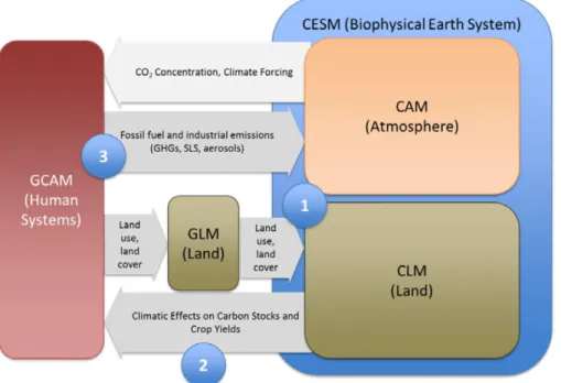
But as sophisticated as this interaction has become, it is still a one-way transfer of information from IAMs to ESMs (Fig. 1). It does not allow IAMs to easily examine the climate system consequences of changes in human decisions as represented in

25

(5)

GMDD

8, 381–427, 2015

Title Page

Tables Figures

◭ ◮

Back Close

Full Screen / Esc

Discussion

P

a

per

|

Discussion

P

a

per

|

Discussion

P

a

per

|

Discussion

P

a

per

system. However, the emerging observable impacts of climate change mean that we can no longer assume that human energy and land systems that produce emissions are evolving under a static climate.

It is therefore clear that future work must enable the processes in these sectors to interact with each other and the climate system rather than remain as one-way transfers

5

of information. If ESMs are to include better representations of the feedbacks of climate change on agriculture, land use, land cover, and terrestrial carbon cycle, as well as other human systems such as energy and the economy, then they will need the ability to incorporate the human system directly. Heretofore the tools have not existed for a fully consistent representation of the combined evolution of these two systems.

10

In order to advance beyond this paradigm, we have developed a new model frame-work, the integrated Earth System Model (iESM). The goal is to create a first-generation integrated system to improve climate simulations and enhance scientific understanding of climate impacts on human systems and important feedbacks from human activities to the climate system. The first version of the iESM described in this paper is designed

15

to address three major science questions: (1) Is the present CMIP5 “parallel process” approach to climate assessment adequate? (2) Will human activities a_ffect local and re-gional climate on scales that matter? (3) Will climate change itself affect global human decision making and biogeochemical and biogeophysical processes?

The iESM is a new configuration of models previously operated separately. The iESM

20

includes the human system components of an integrated assessment model called the Global Change Assessment Model (GCAM) (Kim et al., 2006; Calvin, 2011; Wise et al., 2014), the complete Community Earth System Model (CESM) (Hurrell et al., 2013), and the Global Land-use Model (GLM) (Hurtt et al., 2011) for rendering GCAM output onto the spatial grid and transforming land-use information for use by the Community

25

(6)

GMDD

8, 381–427, 2015

Title Page

Tables Figures

◭ ◮

Back Close

Full Screen / Esc

Discussion

P

a

per

|

Discussion

P

a

per

|

Discussion

P

a

per

|

Discussion

P

a

per

|

The iESM includes both one-way and two-way communication of fluxes and feed-backs among the components of the energy and land-use systems from GCAM, as well as the incorporation of their physical consequences for both biogeochemical and physical fluxes in CESM. This allows the investigation of the degree to which this link-age may change the evolution of the climate system over decades to a century. We

5

have used the integrated Earth System Model (iESM) to investigate the climate im-pacts on human systems and important feedbacks from human activities to the climate system. The iESM results on impacts and feedbacks are described in a series of earlier and companion papers (e.g., Jones et al., 2012, 2013).

This paper describes the scientific rationale for the construction of the iESM (Sect. 2),

10

the component models assembled to create it (Sect. 3), the requirements on the as-sembly process (Sect. 4), the technical implementation of the model (Sect. 5), and the procedures used to validate the linkages among the component models and ensure the integrity of the coupled system (Sect. 6). The paper concludes with future plans for further extensions and applications of the iESM (Sect. 7).

15

2 Climate change impact on energy demand, supply, and production

Climate change can influence energy demand, supply, and production in several major areas. Energy demand for adaptation and mitigation measures may also increase un-der climate change (van Vuuren et al., 2012). Integrated assessment (IA) models can be used to explore consequences and responses of energy systems to climate change.

20

In the IA modeling community, however, energy supply and demand are normally mod-eled based on historical conditions, and climate change impacts are rarely incorpo-rated except in a static manner. Although some e_fforts have begun to explore climate change impacts on the energy system using IA models (Voldoire et al., 2007), only one-way coupling is usually employed, and the interactions between the energy

sys-25

(7)

GMDD

8, 381–427, 2015

Title Page

Tables Figures

◭ ◮

Back Close

Full Screen / Esc

Discussion

P

a

per

|

Discussion

P

a

per

|

Discussion

P

a

per

|

Discussion

P

a

per

energy use, (2) renewable energy potential, and (3) energy production (thermal power plants) and transmission, each of which is described in greater detail below.

2.1 Building energy use

Climate change can have important impacts on building energy systems through de-creased heating and inde-creased cooling. Previous studies are limited in addressing the

5

effect of a changing climate on building energy demands while simultaneously con-sidering other energy sectors in the underlying human systems. In recent years, the impacts of climate change on building energy use have been evaluated using IA mod-els by constructing estimates of heating and cooling degree days from air temperature outputted from climate models (Isaac and van Vuuren, 2009; van Ruijven et al., 2011;

10

Zhou et al., 2013, 2014; Yu et al., 2014). The feedback from the climate on the energy system was calculated from climate model output in advance using a one-way cou-pling scheme, and the impact of these changes in the energy system on climate was rarely considered in these studies. One exception is the study by Labriet et al. (2013), in which the climate change and building energy use was fully coupled with IA and

15

climate models. However, the spatial resolution of climate outputs from this coupled modeling system was low (5◦_{), and it may limit the understanding of climate change}

impact on building energy use.

2.2 Renewable energy production

Renewable energy plays an important role in the energy system at the regional and

20

global levels, and it can be influenced by climate change to a large extent. In current IA modeling efforts, the availability of renewable energy (i.e., wind, solar energy, and hydropower) and its economic potential are either modeled according to the historical condition (Zhang et al., 2010; Zhou et al., 2012) or exogenously quantified using prox-ies such as precipitation or runo_ff(Golombek et al., 2012). However, renewable energy

25

(8)

GMDD

8, 381–427, 2015

Title Page

Tables Figures

◭ ◮

Back Close

Full Screen / Esc

Discussion

P

a

per

|

Discussion

P

a

per

|

Discussion

P

a

per

|

Discussion

P

a

per

|

be very different from current or historical conditions under climate change. For exam-ple, previous studies found that both wind speed and variability show changing trends in the historical time period (Holt and Wang, 2012; Zhou and Smith, 2013) that can impact wind energy potential. Climate change can also alter future photovoltaic and concen-trated solar power energy output through changes in temperature and solar insolation

5

(Crook et al., 2011). Hydropower potential can be influenced by precipitation and runoff

changes under climate change, and previous studies found changes in hydropower po-tential under climate change globally and regionally (Hamududu and Killingtveit, 2012; de Lucena et al., 2009). Interactions between climate change and bioenergy are more complex because of changes in variables such as land use, which will in turn alter

sur-10

face albedo and feedback on the climate (Schae_ffer et al., 2006). The change of future renewable energy under climate change is rarely captured in current IA models, and the subsequent feedback of energy system change on climate systems has not been explored.

2.3 Energy production

15

Climate change also has important impacts on energy production, especially ther-mal power plants, which are influenced by the temperature of water used for cooling (Ruebbelke and Voegele, 2013, 2011) and which might also face limits to water avail-ability in some cases. Increasing air and water temperature under climate change can reduce the efficiency of power plants. For example, it was found in a previous study

20

that a 1◦_{C increase in temperature can reduce the supply of nuclear power by about}

0.5 % (Linnerud et al., 2011). In some extreme cases such as droughts and heat waves, power plants may not be able to meet temporary demand and may even shut down. Moreover, climate change such as extreme weather events and higher temperature also influence transmission lines through disruption of infrastructure or reduction of

25

(9)

GMDD

8, 381–427, 2015

Title Page

Tables Figures

◭ ◮

Back Close

Full Screen / Esc

Discussion

P

a

per

|

Discussion

P

a

per

|

Discussion

P

a

per

|

Discussion

P

a

per

2013). Therefore, these studies of climate change impact on energy production are necessarily limited without a more comprehensive understanding of the human sys-tem. IA models provide the possibility to evaluate the climate change on energy pro-duction in a comprehensive way. For example, a simple assumption has been made to evaluate the climate change impact on thermal efficiency of power plants in the study

5

by Golombek et al. (2012), although there was still no feedback of change in energy system back to the climate in this study.

3 Models

3.1 The Community Earth System Model (CESM)

The starting point for the team’s development efforts was version 1.0 (now 1.1) of the

10

Community Earth System Model (CESM). CESM is a community code and may be downloaded from the Community Earth System Model Project (2014) (URL in refer-ences).

The CESM uses a flexible coupler that couples the atmosphere, ocean, land, and ice component models. Components often use different grids, and the coupler performs

15

the necessary interpolation of fluxes and state variables. The CESM system comprises the Parallel Ocean Program, version 2 (POP), the Community Land Model, version 4.0 (CLM 4.0), the Los Alamos sea-ice model (CICE), the Community Atmosphere Model, version 5 (CAM), and the Community Ice Sheet Model (CISM). POP and CICE are finite volume codes with semi-implicit and explicit time integration and are implemented

20

on logically Cartesian meshes that are stretched to embed polar singularities in land regions and thereby remove these singularities from computation.

The CAM model has flexible formulations for atmospheric dynamics, and it has re-cently transitioned to the spectral finite element method coupled to an extensive suite of sub-grid physical parameterizations in its standard configuration. CAM runs on

un-25

(10)

parameter-GMDD

8, 381–427, 2015

Title Page

Tables Figures

◭ ◮

Back Close

Full Screen / Esc

Discussion

P

a

per

|

Discussion

P

a

per

|

Discussion

P

a

per

|

Discussion

P

a

per

|

izations running at each grid point with no communication between grid points. CLM 4.0 represents surface and subsurface water, energy, carbon, and nitrogen dynamics with a nested hierarchical sub-grid treatment that allows glaciers, lakes, urban areas, agricultural fields, forest, grassland, and shrubland to share space on each grid-cell. In-cident radiation is intercepted in a two-layer canopy, with vegetation, soil, snow aging,

5

and black carbon impacts on albedo. Subsurface processes include vertically resolved biogeochemistry, options for carbon and nutrient cycle parameterization, and recently improved treatment of wetlands and permafrost dynamics. CISM is based upon the Glimmer model, an open source (GPL) three-dimensional thermomechanical ice sheet model designed to be interfaced to a range of global climate models.

10

In the fully-coupled configuration, the CICE and POP component models run with a nominal displaced-pole grid spacing of 1◦ _{(approximately 110 km at the equator and}

30 km in polar regions) and, for POP, 42 levels in the vertical. The CAM and CLM mod-els run with grids with 0.9◦

×1.25◦resolution with 30 and 10 vertical levels, respectively. CLM also includes a separate vegetation layer. The output of the CESM consists of

15

monthly means of several hundred quantities, plus daily averages of a subset of these quantities and hourly output of some key variables.

3.1.1 Development of land-use and land cover change representation in CLM4

A mechanistic representation for the influence of land use and land cover change (LULCC) on carbon, nitrogen, water, and energy cycles was developed and

imple-20

mented for the CMIP5 land-use harmonization (Oleson et al., 2010; Lawrence et al., 2012). This approach is designed to operate on the land-use data stream provided by the GLM code after translation from the four basic land cover types of GLM into the 18 plant functional types (PFTs) of CLM. The CLM LULCC approach recognizes net annual losses and gains of vegetated area for each PFT within each grid cell. Net loss

25

(11)

GMDD

8, 381–427, 2015

Title Page

Tables Figures

◭ ◮

Back Close

Full Screen / Esc

Discussion

P

a

per

|

Discussion

P

a

per

|

Discussion

P

a

per

|

Discussion

P

a

per

extend the existing area and expand the existing biomass to cover the new area. This dynamic LULCC in CLM 4 is one of several anthropogenic forcing factors influencing global biogeochemical cycles and surface energy balance and has been extensively evaluated (Shi et al., 2011, 2013; Mao et al., 2012a, b, 2013).

3.2 The Global Change Assessment Model (GCAM)

5

GCAM is a dynamic-recursive model with technology-rich representations of the econ-omy, energy sector, land use, and water linked to a reduced-form climate model that can be used to explore climate change mitigation policies, including carbon taxes, car-bon trading, regulations and accelerated deployment of energy technology (Edmonds and Reilly, 1985; Kim et al., 2006; Calvin, 2011; Wise et al., 2014). GCAM is a

com-10

munity code and may be downloaded from the Joint Global Change Research Institute (2014) (URL in references).

Regional population and labor productivity growth assumptions drive the energy and land-use systems employing numerous technology options to produce, transform, and provide energy services as well as to produce agriculture and forest products and to

15

determine land use and land cover. Using a run period extending from 1990–2100 at 5-year intervals, GCAM has been used to explore the potential role of emerging energy supply technologies and the greenhouse gas consequences of specific policy measures or energy technology adoption including CO₂ capture and storage, bioen-ergy, hydrogen systems, nuclear enbioen-ergy, renewable energy technology, and energy

20

use technology in buildings, industry and the transportation sectors (e.g. Clarke et al., 2007, 2009).

GCAM is a Representative Concentration Pathway (RCP)-class model. This means it can produce the emissions and land use outputs necessary to force a full AOGCM or ESM as in the CMIP5 process (Thomson et al., 2011). Output includes projections

25

(12)

GMDD

8, 381–427, 2015

Title Page

Tables Figures

◭ ◮

Back Close

Full Screen / Esc

Discussion

P

a

per

|

Discussion

P

a

per

|

Discussion

P

a

per

|

Discussion

P

a

per

|

species at 0.5◦

×0.5◦ resolution, contingent on assumptions about future population, economy, technology, and climate mitigation policy.

For iESM, the time step of GCAM was reduced from 15 to a 5-year standard with flexible time-step capability. This capability is important for scale consistency and com-patibility with CESM code. In addition, the land component, which simulates supply

5

of land products (food, energy, fiber), was completely reformulated to follow functional forms that define productivity as a function of geographic location, climatic conditions, and inputs, and thus made more consistent with physical earth system parameters (Wise and Calvin, 2011). A higher spatial resolution dataset was compiled to allow for land productivity simulation in 151 global regions (Kyle et al., 2011). Finally, the

post-10

processing code to downscale human emissions of CO2 from the GCAM 14-region scale to a CAM-compatible grid was redeveloped and ported to the CESM by the iESM development team. The downscaling of short term forcers is currently under develop-ment.

3.3 The Global Land-Use Model (GLM)

15

The Global Land-Use Model (GLM) is a tool for computing annual, gridded, fractional land-use states and all underlying land-use transitions, including the age, area and biomass of secondary (recovering) lands and the spatial patterns of wood harvest and shifting cultivation, in a format designed for inclusion in Earth System Models (Hurtt et al., 2006). GLM computes these land-use patterns using an accounting-based

20

method that tracks the fractions of cropland, pasture, urban area, primary vegetation, and secondary vegetation in each grid cell as a function of the land surface at the previous time-step. The solution of the model is constrained with inputs and data in-cluding historical reconstructions and future projections of land use (e.g., crop, pasture, and urban applications), wood harvest, and potential biomass and recovery rate. GLM

25

(13)

GMDD

8, 381–427, 2015

Title Page

Tables Figures

◭ ◮

Back Close

Full Screen / Esc

Discussion

P

a

per

|

Discussion

P

a

per

|

Discussion

P

a

per

|

Discussion

P

a

per

GLM was selected as the primary tool to provide harmonized land-use datasets (Hurtt et al., 2011; Brovkin et al., 2013) for the CMIP5 experiments (Taylor et al., 2011) as part of the Fifth IPCC Assessment Report (IPCC, 2014). For this project GLM was used to compute the land-use states and transitions annually, for the years 1500–2100, using data from Integrated Assessment models for the years 1850–2100. GLM

pro-5

vided a continuous time-series of land-use data at half-degree spatial resolution in a format that could be used by a variety of ESMs consistent with both the historical data and future data from IAMs utilizing data from a variety of IAMs. Further information on this application of GLM is available from the Land-use Harmonization Project (2014) (2014; URL in references).

10

For use in iESM, GLM was modified to use GCAM data on a 5-year time-step and to accept data partitioned by GCAM’s 151 agri-ecological zones instead of GCAM’s 14 socioeconomic regions. In addition, GLM was altered to use the forest area data from GCAM and to spatially rearrange agricultural area within each AEZ to match potential forest area changes from GCAM.

15

4 Requirements for the coupling among GCAM, GLM, and CESM1

To ensure that the iESM is reliable, flexible, and extensible, its technical implementation follows from an extensive set of requirements that are detailed below.

4.1 Implementation of iESM as an extension of CESM

The primary goal of the development is to implement the iESM as an extension of the

20

CESM to include a human dimension component. This requirement implies that the integrated assessment model is treated as a new component in CESM and the pro-tocols applied to the five existing components are adopted for the human component as well. To conform with these protocols, the human dimension component has been integrated into CESM’s software environment, including CESM’s configure and build

(14)

GMDD

8, 381–427, 2015

Title Page

Tables Figures

◭ ◮

Back Close

Full Screen / Esc

Discussion

P

a

per

|

Discussion

P

a

per

|

Discussion

P

a

per

|

Discussion

P

a

per

|

procedures, execution protocols, input and output conventions, and regression testing procedures. The execution protocols include CESM’s procedures for synchronizing the coupling and time stepping of its various components and for exchange of fields among these components that conform with the conservation laws (e.g., conservation of mass) governing the dynamic evolution of the whole system.

5

The developers have also ensured that the iESM conforms to CESM’s standards for repeatable experiments, including exact restarts and use of machine-independent representations for the initial, boundary, and restart data sets. CESM has adopted the Network Common Data Format (NetCDF) for these data sets to utilize its features for representation of numerical fields that can be transparently exchanged across

com-10

putational platforms. This is complemented by the requirement that iESM conform to CESM’s standards for hardware and software portability. This requirement helps en-sure that experiments with iESM are, in principle, strictly repeatable assuming that the underlying software and hardware configuration has been validated by the CESM project. In practice, a precise description of the boundary and initial conditions, together

15

with a detailed description of the model and its functionality, are needed to attain ex-perimental reproducibility. To address this need, it follows that the functionality of the human dimensions component should be clearly and comprehensively documented. The documentation should encompass individual pieces such as GCAM, GLM, the Land-use Translator (LUT) code, as well as the pre/post processing code which

oper-20

ates on the data exchanged within the human dimensions component.

4.2 Flexible modes of execution

The second principal goal is to incorporate and extend CESM’s flexible modes of ex-ecution to iESM. The flexibility has two main dimensions: first, the trade-off between the physical completeness and complexity of the model and its execution speed; and

25

(15)

GMDD

8, 381–427, 2015

Title Page

Tables Figures

◭ ◮

Back Close

Full Screen / Esc

Discussion

P

a

per

|

Discussion

P

a

per

|

Discussion

P

a

per

|

Discussion

P

a

per

very simple to very complete representations of the component dynamics, with a cor-responding range from inexpensive to intensive computational resource demands. The second type of flexibility is implemented by introducing versions of each component that either produce the same output state (e.g., a climatology read from data file) regardless of the input state, or that compute an output state based on the input state combined

5

with its evolution equations. The omission or inclusion of two-way communication cor-responds to the omission or inclusion of feedbacks between the given component and the rest of the model system.

Both types of flexibility are realized by incorporating three basic versions of each component known as “stub”, “data”, and “active” versions. The “stub” version is used

10

primarily for automated testing of the system integration and performs some very rudi-mentary housekeeping functions in response to commands from the integration layer of the whole CESM. The “data” version produces a time-evolving state through spatial and/or temporal interpolation applied to a fixed time-dependent input read from data files. The same state is reproduced regardless of the evolution and dynamics of the

15

remainder of the coupled system. This version is computationally inexpensive but does not include the two-way feedbacks between the given component and the rest of the system present in the real world. The “active” version produces a time-evolving state governed by its initial conditions, a representation of the fundamental dynamical equa-tions that pertain to that component, and the boundary condiequa-tions supplied by the rest

20

of the coupled model system. This version is computationally intensive but includes the two-way feedbacks present in the real world.

To conform with this protocol, the iESM includes stub and data version of the hu-man dimensions component, as well as the fully interactive assessment model GCAM. The stub and data versions are automatically tested to ensure that they are integrated

25

(16)

GMDD

8, 381–427, 2015

Title Page

Tables Figures

◭ ◮

Back Close

Full Screen / Esc

Discussion

P

a

per

|

Discussion

P

a

per

|

Discussion

P

a

per

|

Discussion

P

a

per

|

4.3 Bilateral exchange among components of the coupled system

CESM utilizes a set of standard protocols to implement bilateral exchange among com-ponents of the coupled system, and these protocols have been adopted for internal communications within the human component as well as including GCAM, GLM, the LUT code that prepares GLM output for input into CLM, and the associated interfaces.

5

These protocols ensure that the modes of interaction and exchange among compo-nents are visible, reproducible, flexible, and extensible.

The visibility follows from the requirement that all fields are exchanged through a sin-gle, top-level, standardized communication mechanism. This mechanism is capable of recording all information input to and output from all model components, together with

10

the operations performed by the coupling layer to enable the exchanges. This capabil-ity also ensures that the interactions are strictly reproducible, since all exchanges are managed and recorded by one standardized communication mechanism.

This mechanism can be configured at run time to add arbitrary numbers of fields to be exchanged among any given pair of components. This ensures that the

commu-15

nication protocol can support increasingly complete and complex interactions among components using the same well-tested framework, without the need for lengthy modi-fications to the underlying software.

iESM has adopted these conventions for exchanging information to integrate the functional parts within the human dimensions component and, ultimately, to couple the

20

human-dimensions component to other components in CESM. In the first implemen-tation, the data passed between the human dimensions components and the rest of CESM are exchanged using data files to minimize the modifications to the existing CESM components. However, these data exchanges can be readily upgraded to the standard top-level interfaces, internal memory, and message passage adopted by the

25

rest of CESM.

(17)

GMDD

8, 381–427, 2015

Title Page

Tables Figures

◭ ◮

Back Close

Full Screen / Esc

Discussion

P

a

per

|

Discussion

P

a

per

|

Discussion

P

a

per

|

Discussion

P

a

per

protocol (tntcat.iiasa.ac.at:8787/RcpDb/). The information exchanged at the interfaces between the human component and the rest of CESM depend on the precise experi-mental configuration. However, the interfaces themselves are invariant under changes in configuration to guarantee that a single set of communication software can be thor-oughly and repeatedly tested and validated.

5

4.4 Methodologies to treat the ranges in spatial and temporal resolution across iESM

The integrated assessment model solves for the evolution of the human system using a fundamental assumption of market quasi-equilibrium, namely that the inputs and outputs into energy generation, food production, and land resources are balanced on

10

sufficiently large spatial and temporal scales. The length and time scales required for the market equilibrium assumption to hold are orders of magnitude larger than the corresponding scales used to solve the equations of motion for physical, chemical, and biogeochemical processes in the Earth system.

This disparity introduces a requirement on the design of the iESM, namely to

imple-15

ment a flexible and extensible mechanism to handle differences in spatial and temporal resolutions between the human and physical components. To meet this requirement, iESM should include capabilities in temporal interpolation or accumulation (e.g. time averaging, or other operations) in all the interfaces depend on the ratio of time steps between the transmitting and receiving components linked by the interface. Similarly,

20

spatial interpolation or accumulation should be included with the recognition that some preprocessing may be needed to prepare input datafiles to manage regridding.

These capabilities are consolidated into the interfaces among the human component and the rest of the CESM system to avoid “hard wiring” any assumptions about gra-dations in resolutions into the components themselves. The efficient exchange of data

25

(18)

GMDD

8, 381–427, 2015

Title Page

Tables Figures

◭ ◮

Back Close

Full Screen / Esc

Discussion

P

a

per

|

Discussion

P

a

per

|

Discussion

P

a

per

|

Discussion

P

a

per

|

of communication infrastructure that has been optimized to maximize computational throughput. In turn, the exchange of data between components operating on very dif-ferent timesteps introduces a strong dependency on the time management procedures for the whole coupled system. This dependency has been satisfied by completely pre-scribing the sequence of component execution, the interlaced calls to the interfaces,

5

and the interpolation/accumulation operations in each interface call.

While CESM is designed for hybrid execution in any combination of serial and/or par-allel execution of its various components, in the initial version of iESM the human com-ponent is run in serial mode. This mode of operation is necessitated by the multi-year timestep of GCAM. Since the version GCAM used in iESM runs as a single-threaded

10

application while the rest of the CESM is inherently multi-threaded, the processor ele-ments devoted to the non-human components are idle while GCAM is run for a single timestep. This introduces the risk that iESM utilizes computational resources much less e_fficiently than the parent CESM. It is therefore necessary to evaluate the relative cost of the human dimensions component to ensure it is not a performance or memory

15

bottleneck and refactor or parallelize code as needed. Fortunately the overall CESM performance is only marginally impacted by the introduction of this serial code.

4.5 Dual use capability and single code repository for GCAM

GCAM and GLM, like the other components of CESM, are research codes and are therefore under continual development and extension by their primary developers and

20

by the wider GCAM and land-use communities. Recent developments include signifi-cant new capabilities directly relevant to studies of human–Earth system interactions, for example the introduction of supply and demand for water resources (Hejazi et al., 2013, 2014). In order to ensure that the human dimension capabilities of iESM stay current with IA science, the iESM developers have chosen to enhance GCAM and

25

(19)

GMDD

8, 381–427, 2015

Title Page

Tables Figures

◭ ◮

Back Close

Full Screen / Esc

Discussion

P

a

per

|

Discussion

P

a

per

|

Discussion

P

a

per

|

Discussion

P

a

per

or elements of iESM, and these capabilities would be easily propagated to future ver-sions with new scientific features of interest to both the GCAM and iESM communities. These future versions can then be extracted from the respective repositories to easily update iESM.

This design introduces several subsidiary requirements for the input to and output

5

from GCAM and GLM. First, GCAM’s and GLM’s native input and output procedures must be extended as needed to perform file I/O in stand-alone mode to exchange data that is compatible with CESM. This in turn requires introducing input and output in-terfaces into GCAM and GLM that generalize the methods for information exchange to include message passing. As a result, the results from GCAM and GLM are

indis-10

tinguishable whether using files or inline communication techniques to exchange data with the rest of iESM.

4.6 A simplified and robust run-time environment for the GLM component

One of the challenges in constructing iESM is the complexity of the historical land-use and land-cover data required for the downscaling operations performed by GLM. In

15

order to create a much simpler and more robust run-time environment for the GLM component, several important modifications are necessary. These include collating and converting the numerous input and output data sets into a much small number of NetCDF files. It was also helpful to standardize GLM’s control interface to provide a simple and robust way to manage GLM functionality. To reduce the considerable

de-20

(20)

GMDD

8, 381–427, 2015

Title Page

Tables Figures

◭ ◮

Back Close

Full Screen / Esc

Discussion

P

a

per

|

Discussion

P

a

per

|

Discussion

P

a

per

|

Discussion

P

a

per

|

4.7 Reproduction of the offline-coupled implementation of iESM

To the extent feasible, it would be advantageous to have the coupled iESM reproduce the offline-coupled implementation using separate models. To meet this requirement, it is necessary to construct tests ensuring that the data exported by each interface agrees with the corresponding information exchanges in the offline-coupled implementation to

5

the precision of the standalone implementation. In turn, these tests are based upon and therefore require a core level of state output and diagnostics to allow iESM to be validated against relevant observations and documented CESM/GCAM/GLM control runs.

5 Implementation of the coupling among GCAM, GLM, and CESM

10

The first phase of iESM code development was designed to update and codify the experimental protocol from CMIP5 to incorporate land use change and emissions of GHGs and SLS from GCAM into CESM, such that the models exchanged information at each time step rather than as a single, full-century pass at the start of the model future period (2005). The software development team acquired the GCAM and GLM model

15

codes and incorporated them into the land node of CESM through a new component, the Integrated Assessment component (IAC). The IAC is currently visible only to the land model when run in iESM mode and drives prognostic land use change. Because the functionality of GCAM-GLM is encapsulated within a CESM component, it can also be replaced by a data-model, enabling testing with a range of integrated assessment

20

models.

Code modifications were made to GCAM such that the model looks to CESM for instruction on when to begin each new time step. Thus, the first version of the cou-pled model operates by GCAM projecting land use, then CESM projecting climate and ecosystem change and returning productivity information to GCAM, which then

incor-25

(21)

GMDD

8, 381–427, 2015

Title Page

Tables Figures

◭ ◮

Back Close

Full Screen / Esc

Discussion

P

a

per

|

Discussion

P

a

per

|

Discussion

P

a

per

|

Discussion

P

a

per

The code has been tested and is running on leadership-class computing facilities at ORNL (the Titan Cray XK7) and NERSC (the Hopper Cray XE6 and Edison Cray XC30) and has also been tested and configured on the DOE IARP cluster at PNNL/UMD (Evergreen). The iESM code has also kept pace with current CESM versions, and was most recently updated (in summer 2013) to run with CESM 1.1.2, the most recent

5

CESM release with a full carbon cycle spin-up available.

Scientific challenges were encountered in the design of the coupling between CESM and the IAC component, specifically with regard to faithfully representing CESM’s land productivity passed into the IAC as well as capturing the land-use change being re-turned. These challenges were identified and solved through a series of soft-coupled

10

runs where the project team ran each model one time-step forward at a time and passed model output between them, as well as a series of offline, CLM-only runs with the IAC enabled. In this fashion, the coupling steps were refined while the software development was under way. This first development phase focused on the land-use change components of the models. In parallel, algorithms to downscale GCAM GHG

15

and SLS emissions have been developed and tested, and the code has been trans-ferred to the development team.

5.1 General IAC implementation

The IAC is implemented like a standard component of CESM. The IAC component has stub, data, and active versions called SIAC, DIAC, and GIAC, respectively, that

20

provide a range of functionalities and capabilities for the IAC component. The active IAC version (GIAC) is fully prognostic and runs the full suite of IAC subcomponents to produce dynamically varying land use/change data using carbon feedback scalars from CLM. The data component (DIAC) replaces the active GCAM/GLM submodels with data derived from an offline IAM/GLM control run. It is currently used for testing

25

(22)

GMDD

8, 381–427, 2015

Title Page

Tables Figures

◭ ◮

Back Close

Full Screen / Esc

Discussion

P

a

per

|

Discussion

P

a

per

|

Discussion

P

a

per

|

Discussion

P

a

per

|

model, namely to serve as a placeholder to satisfy interface requirements when the active or data component is not being run. The stub IAC is the default mode for CLM, which makes it 100 % bit-for-bit backward compatible with the current CLM.

Like other CESM components, IAC has routines to initialize its state, execute by evolving forward in time, and complete its operations by communicating its new state

5

and generating history and restart (check-point) files. While these routines do not sat-isfy all aspects of the current CESM interface standard, they could be readily modified to do so in the future. The checkpoint/restart mechanism built for the IAC meets the CESM requirements for exact restarts to facilitate long integrations of the model sys-tem. Following the template of other CESM components, the IAC has a built-in clock,

10

a top-level interface that mimics a CESM component, a centralized collection of control information implemented via a standard Fortran namelist, and a set of clock, grid, con-trol and field parameters defined in a shared module for query by and exchange with other parts of the model system. All the coupling within the IAC is done via internal memory.

15

While the IAC was initially implemented as a separate component in CESM, we have placed the IAC component beneath the land model, since the all the coupling in the initial version of iESM would involve the CESM land component. Because we are using a mature coupling strategy, we can easily reposition the IAC component as needed in the future. But for the moment, the IAC is implemented as an option in CLM,

20

and therefore the IAC model resides in its own subdirectory within the main code base for CLM. The stub, active, or data mode of IAC is set via the CESM configuration files. When this mode is set to stub, the results from iESM are identical at the bit-for-bit level with the corresponding version of the conventional CESM. All the input data sets and namelist parameters for the IAC are set by enhanced versions of the

namelist-25

generation procedures for CLM.

(23)

GMDD

8, 381–427, 2015

Title Page

Tables Figures

◭ ◮

Back Close

Full Screen / Esc

Discussion

P

a

per

|

Discussion

P

a

per

|

Discussion

P

a

per

|

Discussion

P

a

per

specified by the user. Most of the IAC code is written in Fortran 90 or C, and leverages the CESM makefile. When the active IAC model is specified, GCAM is built via GCAM’s build scripts that have been modified slightly to support coupling while retaining support for GCAM’s implementation in C++. Currently, coupling between the IAC and CLM components is done via data files to leverage current CLM capabilities and to minimize

5

changes to CLM. The IAC reads data from CLM history files at the start of a time step and writes data to a time varying surface data set at the end of the IAC timestep. Both sets of data evolve in time as the coupled system advances.

5.2 IAC design

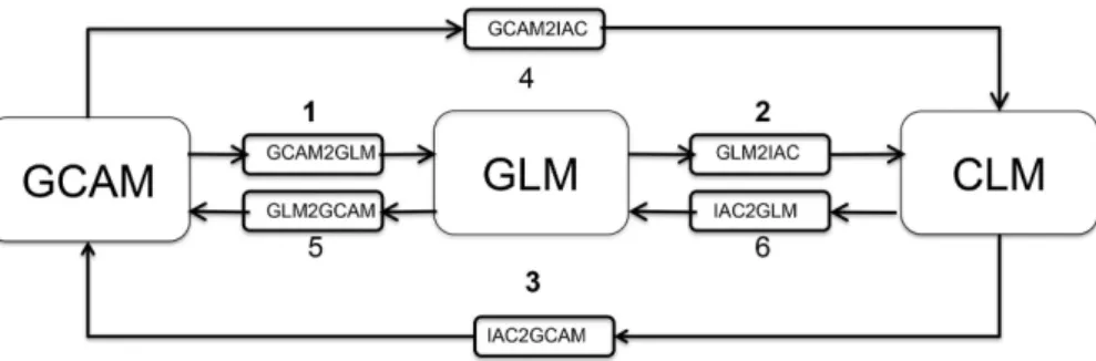
The IAC component consists of five subcomponents, including the models GCAM and

10

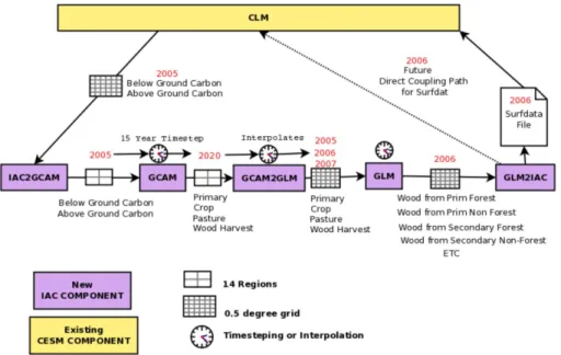
GLM and the interfaces IAC2GCAM, GCAM2GLM, and GLM2IAC between these mod-els and the rest of the IAC component (Fig. 3). The sequence in which these subcom-ponents is invoked starts with IAC2GCAM, proceeds through GCAM, GCAM2GLM, and GLM, and concludes with GLM2IAC. Each sub-model is called in turn, process-ing CLM carbon information at the beginnprocess-ing of the sequence and eventually

pro-15

ducing an updated land state that will be read by CESM throughout the model year (Fig. 4). The computational load of the IAC is dominated by GCAM and GLM, with the remaining subcomponents handling the processing needed to connect those models to each other and the rest of CESM. The IAC component includes the capability to read and write data between each step, thereby facilitating validation of each piece of

20

(24)

GMDD

8, 381–427, 2015

Title Page

Tables Figures

◭ ◮

Back Close

Full Screen / Esc

Discussion

P

a

per

|

Discussion

P

a

per

|

Discussion

P

a

per

|

Discussion

P

a

per

|

5.3 IAC2GCAM

The IAC2GCAM interface translates and remaps gridded information from CLM on its terrestrial carbon state into regional scaling factors (scalars) for crop yields and ecosys-tem carbon densities used by the agriculture and land-use module internal to GCAM (Bond-Lamberty et al., 2014). The scalars represent our initial attempt to reconcile the

5

separate carbon inventories either explicitly computed by or implicitly embedded via boundary data in the CLM, GCAM, GLM and interface routines. In this initial version of iESM, the input to IAC2GCAM is read from CLM history files and includes the fields listed in Table 1. The output consists of scalar fields for 27 crop and land-cover fields on each of GCAM’s 151 land units. The remapping between the CLM grid and GCAM

10

regions is accomplished by translating CLM carbon, defined in broad terms of vegeta-tive functional types, to the 27 specific GCAM crop/land types that lie at the heart of its economic, energy and land-use parameterizations. In addition to mapping between different land representations, IAC2GCAM also handles the temporal interpolation and spatial aggregation that is needed to represent CLM’s gridded data in terms of the

an-15

nually averaged regional values that GCAM requires. The spatial regridding process is aided by an external data file that specifies the areal overlap of CLM grid points with the GCAM land units. The mapping of CLM carbon to scalars applied to GCAM above and below-ground carbon is accomplished by averaging over the GCAM time step and then post processing to remove outliers (Bond-Lamberty et al., 2014).

20

5.4 GCAM

The GCAM model produces worldwide land-use projections incorporating informa-tion about demographics, economics, resources, energy producinforma-tion, and consumpinforma-tion (Sect. 3.3.2). Integration into iESM requires modifications to GCAM, including the ad-dition of lightweight interface routines to CESM and the provision to share data in its

25

(25)

GMDD

8, 381–427, 2015

Title Page

Tables Figures

◭ ◮

Back Close

Full Screen / Esc

Discussion

P

a

per

|

Discussion

P

a

per

|

Discussion

P

a

per

|

Discussion

P

a

per

rest of the IAC component comprises the land surface areas for crop, pasture, forest, and the amount of harvested wood carbon for each of GCAM’s 151 land units.

5.5 GCAM2GLM

The GCAM2GLM interface serves to allocate GCAM output from 151 land units to the 0.5◦_{GLM grid. In the process, it also harmonizes the GCAM output to provide a smooth}

5

transition from historical land-use data to future projections. The harmonization and re-gridding algorithms are based upon GLM historical simulations and the 2005 HYDE 3.0 historical land use data set (Klein Goldewijk et al., 2011). The inputs into the in-terface are the projections of crop, pasture, and forest area, as well as the amount of harvested wood carbon for 151 GCAM land units at the 5-year GCAM timestep. The

10

outputs from the interface are the areal extents of cropland, pasture, and forest at an-nual time steps on the GLM half-degree grid, together with a pre-processed version of the wood harvest data readied for spatial allocation within GLM. The GCAM2GLM processing is contingent on the climate-change scenario under consideration and has embedded priorities for how the fractional areas of crop, pasture, and forested land are

15

allocated. For example, these priorities could dictate that agricultural expansion hap-pens preferentially on forested lands. A mechanism for recording and readily altering these embedded allocation priorities should be included in future versions of iESM.

5.6 GLM

In terms of its interactions with the rest of the current IAC components, the GLM model

20

converts the annualized fractional land-use states output by GCAM2GLM into gridded data sets suitable for input into CLM, while also computing the spatial pattern of wood harvest area and the area of natural vegetation occupied by both primary and sec-ondary vegetation. GLM converts the GCAM2GLM output data into a variety of fields on its native half-degree grid, nine of which are currently utilized in iESM including five

(26)

GMDD

8, 381–427, 2015

Title Page

Tables Figures

◭ ◮

Back Close

Full Screen / Esc

Discussion

P

a

per

|

Discussion

P

a

per

|

Discussion

P

a

per

|

Discussion

P

a

per

|

wood-harvest categories (Table 2). GLM also calculates gross land-use/cover transi-tions within each year, but these are not used by CESM.

Integration into CESM has required extensive modifications to GLM, including the re-design of data structures to reduce memory requirements and to accommodate control by CESM of its temporal evolution. Other modifications include the addition of restart

5

functionality, the introduction of a control interface, the conversion of all boundary data into NetCDF, and the provision for routing all input and output through the calling inter-face.

5.7 GLM2IAC

The GLM2IAC interface is tasked with converting the harmonized outputs of GLM to

10

time-varying data sets for land cover and wood-harvest area in CLM’s native input format. The translation of GLM state and harvest variables to CLM land cover is based on code (Lawrence et al., 2012) to process the CMIP5 RCPs (Moss et al., 2010; van Vuuren et al., 2011), as well as on the external tool called mksurfdat (a contraction of “make surface data”) used to generate CLM boundary data for the standard CESM.

15

Both codes were inlined into the IAC component and are run interactively. The original land translation code has been extensively modified to better capture the afforestation signal generated in GCAM and has been renamed the Land Use Translator (Di Vittorio et al., 2014).

5.8 CLM modifications

20

Although CLM and the rest of CESM require minimal modifications to incorporate the IAC component, CLM was modified to permit updates to its time varying input sur-face data sets after its initialization phase. This modification required introducing some changes in order to reread the time axis of the dynamic surface data set during the execution phase of CLM.

(27)

GMDD

8, 381–427, 2015

Title Page

Tables Figures

◭ ◮

Back Close

Full Screen / Esc

Discussion

P

a

per

|

Discussion

P

a

per

|

Discussion

P

a

per

|

Discussion

P

a

per

5.9 Time stepping

The IAC component advances in one-year time steps and is called at the start of each calendar year. During this call, every sub-subcomponent in the IAC component is exe-cuted in order to prognose the time-varying CLM land surface data sets starting from the current CESM time step and ending one year into the future. To accomplish this,

5

the IAC calculates the land surface for the time step one ahead, then CLM interpo-lates between the current and future land surface at its native 30 min time step. In between the yearly IAC timesteps, the IAC component is called monthly from CLM to create an annual average of CLM NPP and HR values. The GCAM subcomponent can be integrated using either one or three sequential 5-year time steps. The default is to

10

use a 5-year time step and interpolate the yearly data needed for the rest of the IAC sub-components. Prior to each GCAM call, the IAC computes the carbon scalars that constitute the feedback between CESM and GCAM.

5.10 Technical issues

Several technical requirements and protocols specific to large climate codes and CESM

15

had to be introduced with the IAC component. The IAC component is bit-for-bit repro-ducible when rerun, and it restarts exactly from check-point files generated by previous runs. The IAC component is included in the CESM code repository and is tagged reg-ularly in order to track code versions. A specific numerical experiment using the IAC in CESM can be described by specifying the model tag, the compset (which determines

20

the model components), the grid, and a set of plain-text files that specify the features and input setting for the CESM components. The CESM configuration scripts have been augmented for iESM to include new compsets and new XML environment vari-ables that specify items like the IAC mode (stub, data, active). The scripts have been further enhanced to incorporate several new libraries required by GCAM to support

25

(28)

GMDD

8, 381–427, 2015

Title Page

Tables Figures

◭ ◮

Back Close

Full Screen / Esc

Discussion

P

a

per

|

Discussion

P

a

per

|

Discussion

P

a

per

|

Discussion

P

a

per

|

These libraries include Berkeley DB XML, Berkeley DB, XQilla, and Xerces C++, which must be installed before the active IAC component can be run within CESM.

To facilitate running the IAC with different CLM grids, many of the IAC settings are specified via namelist or read from files specified at run time. All the output data is written in NetCDF to ensure portability across computing platforms and to exploit the

5

self-documenting features provided by this format. All variables are given explicit types, real variables are assigned to a type of double precision wherever possible, and the Fortran code complies with the CESM coding standard and is written in Fortran 90. Because the GLM and GCAM are written in C and C++, Fortran/C interfaces have been implemented in several parts of the IAC component.

10

6 Validation of the coupling among GCAM, GLM, and CESM

One of the core requirements of the iESM design is to reproduce simulations conducted with the offline-coupled version of the same codes. Satisfaction of this requirement im-plies that the online-coupled simulations with iESM would be statistically indistinguish-able from the offline-coupled simulations. Since the offline-coupled experiments have

15

been configured to emulate the large number of simulations conducted using the same suite of codes for the CMIP5, successful reproduction of the offline-coupled runs would mean that the iESM user community could employ the large literature analyzing the CMIP5 runs to understand the baseline (or control) climatology and climate dynamics of iESM. Since iESM includes a variety of bug fixes and enhancements relative to the

20

offline-coupled model configurations, the emulation will be only approximate.

The tests to verify the degree to which iESM reproduces the offline-coupled model have been conducted in three stages. First, with the exception of GLM, each compo-nent in iESM has been checked separately to show that, given the same input, the output of that component matches that of the corresponding component in the offl

ine-25