and Noise Correlations in Neural Population Codes
Yu Hu1*, Joel Zylberberg1, Eric Shea-Brown1,2,3
1Department of Applied Mathematics, University of Washington, Seattle, Washington, United States of America,2Program in Neurobiology and Behavior, University of Washington, Seattle, Washington, United States of America,3Department of Physiology and Biophysics, University of Washington, Seattle, Washington, United States of America
Abstract
Over repeat presentations of the same stimulus, sensory neurons show variable responses. This ‘‘noise’’ is typically correlated between pairs of cells, and a question with rich history in neuroscience is how these noise correlations impact the population’s ability to encode the stimulus. Here, we consider a very general setting for population coding, investigating how information varies as a function of noise correlations, with all other aspects of the problem – neural tuning curves, etc. – held fixed. This work yields unifying insights into the role of noise correlations. These are summarized in the form of theorems, and illustrated with numerical examples involving neurons with diverse tuning curves. Our main contributions are as follows. (1) We generalize previous results to prove asign rule(SR) — if noise correlations between pairs of neurons have opposite signs vs. their signal correlations, then coding performance will improve compared to the independent case. This holds for three different metrics of coding performance, and for arbitrary tuning curves and levels of heterogeneity. This generality is true for our other results as well. (2) As also pointed out in the literature, the SR does not provide a necessary condition for good coding. We show that a diverse set of correlation structures can improve coding. Many of these violate the SR, as do experimentally observed correlations. There is structure to this diversity: we prove that the optimal correlation structures must lie on boundaries of the possible set of noise correlations. (3) We provide a novel set of necessary and sufficient conditions, under which the coding performance (in the presence of noise) will be as good as it would be if there were no noise present at all.
Citation:Hu Y, Zylberberg J, Shea-Brown E (2014) The Sign Rule and Beyond: Boundary Effects, Flexibility, and Noise Correlations in Neural Population Codes. PLoS Comput Biol 10(2): e1003469. doi:10.1371/journal.pcbi.1003469
Editor:Jonathan W. Pillow, The University of Texas at Austin, United States of America ReceivedAugust 22, 2013;AcceptedDecember 17, 2013;PublishedFebruary 27, 2014
Copyright:ß2014 Hu et al. This is an open-access article distributed under the terms of the Creative Commons Attribution License, which permits unrestricted use, distribution, and reproduction in any medium, provided the original author and source are credited.
Funding:Supported for this work came from NSF CRCNS grant DMS-1208027 and a Career Award at the Scientific Interface from the Burroughs-Wellcome Fund to ESB. The funders had no role in study design, data collection and analysis, decision to publish, or preparation of the manuscript.
Competing Interests:The authors have declared that no competing interests exist. * E-mail: [email protected]
Introduction
Neural populations typically show correlated variability over repeat presentation of the same stimulus [1–4]. These are called noise correlations, to differentiate them from correlations that arise when neurons respond to similar features of a stimulus. Suchsignal correlationsare measured by observing how pairs of mean (averaged over trials) neural responses co-vary as the stimulus is changed [3,5].
How do noise correlations affect the population’s ability to encode information? This question is well-studied [3,5–16], and prior work indicates that the presence of noise correlations can either improve stimulus coding, diminish it, or have little effect (Fig. 1). Which case occurs depends richly on details of the signal and noise correlations, as well as the specific assumptions made. For example [8,9,14] show that a classical picture — wherein positive noise correlations prevent information from increasing linearly with population size — does not generalize to heteroge-neously tuned populations. Similar results were obtained by [17], and these examples emphasize the need for general insights.
Thus, we study a more general mathematical model, and investigate how coding performance changes as the noise correlation are varied. Figure 1, modified and extended from [5], illustrates this process. In this figure, the only aspect of the
population responses that differs from case to case are the noise correlations, resulting in differently shaped distributions. These different noise structures lead to different levels of stimulus discriminability, and hence coding performance. The different cases illustrate our approach: given any set of tuning curves and noise variances, we study how encoded stimulus information varies with respect to the set of all pairwise noise correlations.
Compared to previous work in this area, there are two key differences that makes our analysis novel: we make no particular assumptions on the structure of the tuning curves; and we do not restrict ourselves to any particular correlation structure such as the ‘‘limited-range’’ correlations often used in prior work [5,7,8]. Our results still apply to the previously-studied cases, but also hold much more generally. This approach leads us to derive mathematical theorems relating encoded stimulus information to the set of pairwise noise correlations. We prove the same theorems for several common measures of coding performance: the linear Fisher information, the precision of the optimal linear estimator (OLE [18]), and the mutual information between Gaussian stimuli and responses.
converse is not true, noise correlations that perfectly violate the SR –and thus have the same signs as the signal correlations – can yield better coding performance than does independent noise. Thus, as previously observed [8,9,14], the SR does not provide a necessary condition for correlations to enhance coding performance.
Since experimentally observed noise correlations often have the same signs as the signal correlations [3,6,19], new theoretical insights are needed. To that effect, we develop a new organizing principle: optimal coding will always be obtained on the boundary of the set of allowed correlation coefficients. As we discuss, this boundary can be defined in flexible ways that incorporate constraints from statistics or biological mechanisms.
Finally, we identify conditions under which appropriately chosen noise correlations can yield coding performance as good as would be obtained with deterministic neural responses. For large populations, these conditions are satisfied with high probability, and the set of such correlation matrices is very high-dimensional. Many of them also strongly violate the SR.
Results
The layout of our Results section is as follows. We will begin by describing our setup, and the quantities we will be computing, in Section ‘‘Problem setup’’.
In Section ‘‘The sign rule revisited’’, we will then discuss our generalized version of the ‘‘sign rule’’, Theorem 1, namely that signal and noise correlations between pairs of neurons with opposite signs will always improve encoded information compared with the independent case. Next, in Section ‘‘Optimal correlations lie on boundaries’’, we use the fact that all of our information quantities are convex functions of the noise correlation coefficients to conclude that the optimal noise correlation structure must lie on the boundary of the allowed set of correlation matrices, Theorem 2.
We will further observe that there will typically be a large set of correlation matrices that all yield optimal (or near-optimal) coding performance, in a numerical example of heterogeneously tuned neural populations in Section ‘‘Heterogeneously tuned neural populations’’.
We prove that these observations are general in Section ‘‘Noise cancellation’’ by studying the noise canceling correlations (those that yield the same high coding fidelity as would be obtained in the absence of noise). We will provide a set of necessary and sufficient conditions for correlations to be ‘‘noise canceling’’, Theorem 3, and for a system to allow for these noise canceling correlations, Theorem 4. Finally, we will prove a result that suggests that, in large neural populations with randomly chosen stimulus response characteristics, these conditions are likely to be satisfied, Theorem 5.
A summary of most frequent notations we use is listed in Table 1.
Problem setup
We will consider populations of neurons that generate noisy responses~xxin response to a stimulus~ss. The responses,~xx– wherein each component xi represents one cell’s response – can be
considered to be continuous-valued firing rates, discrete spike counts, or binary ‘‘words’’, wherein each neuron’s response is a 1 (‘‘spike’’) or 0 (‘‘not spike’’). The only exception is that, when we consider Imut,G (discussed below), the responses must be
contin-uous-valued. We consider arbitrary tuning for the neurons;
mi~EfxiD~ssg. For scalar stimuli, this definition of ‘‘tuning’’
corresponds to the notion of a tuning curve. In the case of more complex stimuli, it is similar to the typical notion of a receptive field. Recall that the signal correlations are determined by the co-variation of the mean responses of pairs of neurons as the stimulus is varied, and thus they are determined by the similarity in the tuning functions.
As for the structure of noise across the population, our analysis allows for the general case in which the noise covariance matrix Cn
ij~covxi,xjD~ss(superscriptndenotes ‘‘noise’’) depends on the
stimulus~ss. This generality is particularly interesting given the observations of Poisson-like variability [20,21] in neural systems, and that correlations can vary with stimuli [3,16,19,22]. We will assume that the diagonal entries of the conditional covariance matrix – which describe each cells’ variance – will be fixed, and then ask how coding performance changes as we vary the off-diagonal entries, which describe the covariance between the cell’s responses (recall that the noise correlations are the pairwise covariances, divided by the geometric mean of the relevant variancesrij~Cijn=
ffiffiffiffiffiffiffiffiffiffiffiffi Cn
iiCjjn p
).
We quantify the coding performance with the following measures, which are defined more precisely in the Methods Section ‘‘Defining the information quantities, signal and noise correlations’’, below. First, we consider the linear Fisher informa-tion (IF,lin, Eq. (5)), which measures how easy it is to separate the
response distributions that result from two similar stimuli, with a linear discriminant. This is equivalent to the quantity used by [11] and [10] (where Fisher information reduces toIF,lin). While Fisher
information is a measure oflocalcoding performance, we are also interested in global measures.
We will consider two such global measures, the OLE informationIOLE (Eq. (12)) and mutual information for Gaussian
stimuli and responsesImut,G (Eq. (13)).IOLE quantifies how well
the optimal linear estimator (OLE) can recover the stimulus from the neural responses: large IOLE corresponds to small mean
squared error of OLE and vice versa. For the OLE, there is one set of read-out weights used to estimate the stimulus, and those weights do not change as the stimulus is varied. For contrast, with linear Fisher information, there is generally a different set of weights used for each (small) range of stimuli within which the discrimination is being performed.
Author Summary
Consequently, in the case of IOLE and Imut,G, we will be
considering the average noise covariance matrix Cn
ij~cov(xi,xj) ~E cov xi,xjD~ss
, where the expectation is taken over the stimulus distribution. Here we overload the notation Cn be the
covariance matrix that one chooses during the optimization, which will be either local (conditional covariances at a particular stimulus) or global depending on the information measure we consider.
WhileIOLE and IF,lin are concerned with the performance of
linear decoders, the mutual information Imut,G between stimuli
and responses describes how well the optimal read-out could recover the stimulus from the neural responses, without any assumptions about the form of that decoder. However, we emphasize that our results forImut,Gonly apply to jointly Gaussian
stimulus and response distributions, which is a less general setting
than the conditionally Gaussian cases studied in many places in the literature. An important exception is that Theorem 2 additionally applies to the case of conditionally Gaussian distributions (see discussion in Section ‘‘Convexity of information measures’’).
For simplicity, we describe most results for scalar stimulussif not stated otherwise, but the theory holds for multidimensional stimuli (see Methods Section ‘‘Defining the information quantities, signal and noise correlations’’).
The sign rule revisited
Arguments about pairs of neurons suggest that coding performance is improved – relative to the case of independent, or trial-shuffled data – when the noise correlations have the
Figure 1. Different structures of correlated trial-to-trial variability lead to different coding accuracies in a neural population. (Modified and extended from [5].) We illustrate the underlying issues via a three neuron population, encoding two possible stimulus values (yellow and blue). Neurons’ mean responses are different for each stimulus, representing their tuning. Trial-to-trial variability (noise) around these means is represented by the ellips(oid)s, which show 95% confidence levels. This noise has two aspects: for each individual neuron, its trial-to-trial variance; and at the population level, the noise correlations between pairs of neurons. We fix the former (as well as mean stimulus tuning), and ask how noise correlations impact stimulus coding. Different choices (A–D) of noise correlations affect the orientation and shape of response distributions in different ways, yielding different levels of overlap between the full (3D) distributions for each stimulus. The smaller the overlap, the more discriminable are the stimuli and the higher the coding performance. We also show the 2D projections of these distributions, to facilitate the comparison with the geometrical intuition of [5]. First, RowAis the reference case where neurons’ noise is independent: zero noise correlations. Row Billustrates how noise correlations can increase overlap and worsen coding performance. RowCdemonstrates the opposite case, where noise correlations are chosen consistently with the sign rule (SR) and information is enhanced compared to the independent noise case. Intriguingly, Row Ddemonstrates that there are more favorable possibilities for noise correlations: here, these violate the SR, yet improve coding performance vs. the independent case. Detailed parameter values are listed in Methods Section ‘‘Details for numerical examples and simulations’’.
opposite sign from the signal correlations [5,7,10,13]: we dub this the ‘‘sign rule’’ (SR). This notion has been explored and demonstrated in many places in the experimental and theoretical literature, and formally established for homogenous positive correlations [10]. However, its applicability in general cases is not yet known.
Here, we formulate this SR property as a theorem without restrictions on homogeneity or population size.
Theorem 1. If, for each pair of neurons, the signal and noise correlations have opposite signs, the linear Fisher information is greater than the case of independent noise (trial-shuffled data). In the opposite situation where the signs are the same, the linear Fisher information is decreased compared to the independent case, in a regime of very weak correlations. Similar results hold forIOLEandImut,G, with a modified definition of signal correlations given in
Section. ‘‘Defining the information quantities, signal and noise correlations’’.
In the case of Fisher information, the signal correlation between two neurons is defined asrsigij ~ +mi:+mj
E+miE2E+mjE2 (Section ‘‘Defining the information quantities, signal and noise correlations’’). Here, the derivatives are taken with respect to the stimulus. This definition recalls the notion of the alignment in the change in the neurons’ mean responses in, e.g., [11]. It is important to note that this definition for signal correlation is locally defined near a stimulus value; thus, it differs from some other notions of ‘‘signal correlation’’ in the literature, that quantify how similar the whole tuning curves are for two neurons (see discussion on the alternative
~ r
rsigij in Section ‘‘Defining the information quantities, signal and noise correlations’’). We choose to define signal correlations for IF,lin, IOLE and Imut,G as described in Section ‘‘Defining the
information quantities, signal and noise correlations’’ to reflect precisely the mechanism behind the examples in [5], among others.
It is a consequence of Theorem 1 that the SR holds pairwise; different pairs of neurons will have different signs of noise correlations, as long as they are consistent with their (pairwise) signal correlations. The result holds as well for heterogenous populations. The essence of our proof of Theorem 1 is to calculate the gradient of the information function in the space of noise
correlations. We compute this gradient at the point representing the case where the noise is independent. The gradient itself is determined by the signal correlations, and will have a positive dot product with any direction of changing noise correlations that obeys the sign rule. Thus, information is increased by following the sign rule, and the gradient points to (locally) the direction for changing noise correlations that maximally improves the infor-mation, for a given strength of correlations. A detailed proof is included in Methods Section ‘‘Proof of Theorem 1: the generality of the sign rule’’; this includes a formula for the gradient direction (Remark 1 in Section ‘‘Proof of Theorem 1: the generality of the sign rule’’). We have proven the same result for all three of our coding metrics, and for both scalar, and multi-dimensional, stimuli.
Intriguingly, there exists an asymmetry between the result on improving information (above), and the (converse) question of what noise correlations are worst for population coding. As we will show later, the information quantities are convex functions of the noise correlation coefficients (see Fig. 2). As a consequence, Table 1.Notations.
~ss stimulus
xi response of neuroni mi mean response of neuroni
+mi derivative against~ss, Eq. (6)
L covariance betweenxand~ss, Eq. (11)
Cn noise covariance matrix (averaged or conditional, Section
‘‘Summary of the problem set-up’’) Cm covariance of the mean response, Eq. (10)
]0, 0 (a matrix is) positive definite and positive semidefinite
C~CmzCn total covariance,Eq. (10)
A~C{1L optimal readout vector of OLE, Eq. (9)
rij noise correlations, Eq. (15)
rsig
ij signal correlations, Eq. (16)
IF,lin linear Fisher information, Eq. (5) IOLE OLE information (accuracy of OLE), Eq. (12) Imut,G mutual information for Gaussian distributions, Eq. (13)
doi:10.1371/journal.pcbi.1003469.t001
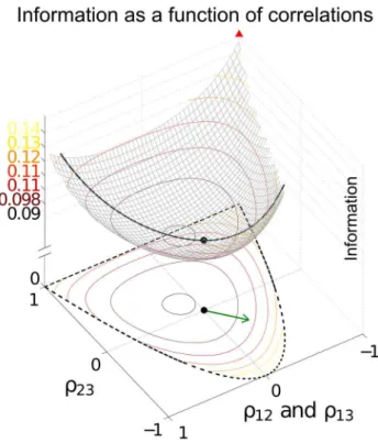
Figure 2. The ‘‘sign rule’’ may fail to identify the globally optimal correlations.The optimal linear estimator (OLE) information
IOLE(Eq. (12)), which is maximized when the OLE produces
minimum-variance signal estimates, is shown as a function of all possible choices of noise correlations (enclosed within the dashed line). These values are
Cn
1,2~C1,3n (x-axis) andC2,3n (y-axis) for a 3-neuron population. The bowl
shape exemplifies the general fact thatIOLEis a convex function and
thus must attain its maximum on the boundary (Theorem 2) of the allowed region of noise correlations. The independent noise case and global optimal noise correlations are labeled by a black dot and triangle respectively. The arrow shows the gradient vector ofIOLE, evaluated at
zero noise correlations. It points to the quadrant in which noise correlations and signal correlations have opposite signs, as suggested by Theorem 1. Note that this gradient vector, derived from the ‘‘sign rule’’, does not point towards the global maximum, and actually misses the entire quadrant containing that maximum. This plot is a two-dimensional slice of the cases considered in Fig. 3, while restricting
Cn
1,2~C1,3n (see Methods Section ‘‘Details for numerical examples and
performance will keep increasing as one continues to move along a ‘‘good’’ direction, for example indicated by the SR. This is what one expects when climbing a parabolic landscape in which the second derivative is always nonnegative. The same convexity result indicates that the performance will not decrease monotonically along a ‘‘bad’’ direction, such as the anti-SR direction. For example, if, while following the anti-SR direction, the system passed by the minimum of the information quantity, then continued increases in correlation magnitude would yield increases in the information. In fact, it is even possible for anti-SR correlations to yield better coding performance than would be achieved with independent noise. An example of this is shown in Fig. 2, where the arrow points in the direction in correlation space predicted by the SR, but performance that is better than with independent noise can also be obtained by choosing noise correlations in the opposite direction.
Thus, the result that anti-SR noise correlations harm coding is only a ‘‘local’’ result – near the point of zero correlations – and therefore requires the assumption of weak correlations. We emphasize that this asymmetry of the SR is intrinsic to the problem, due to the underlying convexity.
One obvious limitation of Theorem 1 and the ‘‘sign rule’’ results in general is that they only compare information in the presence of correlated noise with the baseline case of independent noise. This approach does not address the issue of finding the optimal noise correlations, nor does it provide much insight into experimental data that do not obey the SR. Does the sign rule rule describe optimal configurations? What are the properties of the global optima? How should we interpret noise correlations that do not follow the SR? We will address these questions in the following sections.
Optimal correlations lie on boundaries
Let us begin by considering a simple example to see what could happen for the optimization problem we described in Section ‘‘Problem setup’’, when the baseline of comparison is no longer restricted to the case of independent noise. This example is for a population of 3 neurons. In order to better visualize the results, we further require that Cn
1,2~Cn1,3. Therefore the configurations of
correlations is two dimensional. In Fig. 2, we plot information IOLE as a function of the two free correlation coefficients (in this
example the variances are allCn
ii~1, thusCnij~rij).
First, notice that there is a parabola-shaped region of all attainable correlations (in Fig. 2, enclosed by black dashed lines and the upper boundary of the square). The region is determined not only by the entry-wise constraintDri,jDƒ1(the square), but also
by a global constraint that the covariance matrix Cn must be
positive semidefinite. For linear Fisher information and mutual information for Gaussian distributions, we further assumeCn]0
(i.e.Cnis positive definite) so thatI
F,lin and Imut,G remain finite
(see also Section ‘‘Defining the information quantities, signal and noise correlations’’). As we will see again below, this important constraint leads to many complex properties of the optimization problem. This constraint can be understood by noting that correlations must be chosen to be ‘‘consistent’’ with each other and cannot be freely and independently chosen. For example, if
r1,2~r1,3 are large and positive, then cells 2 and 3 will be
positively correlated – since they both covary positively with cell 1 – andr2,3 may thus not take negative values. In the extreme of r1,2~r1,3~1,r2,3is fully determined to be 1. Cases like this are
reflecting the corner shape in the upper right of the allowed region in Fig. 2.
The case of independent noise is denoted by a black dot in the middle of Fig. 2, and the gradient vector of IOLE points to a
quadrant that is guaranteed to increase information vs. the independent case (Theorem 1). The direction of this gradient satisfies the sign rule, as also guaranteed by Theorem 1. However, the gradient direction and the quadrant of the SR both fail to capture the globally optimal correlations, which are at upper right corner of the allowed region, and indicated by the red triangle. This is typically what happens for larger, and less symmetric populations, as we will demonstrate next.
Since the sign rule cannot be relied upon to indicate the global optimum, what other tools do we have at hand? A key observation, which we prove in the Methods Section ‘‘Proof of Theorem 2: optima lie on boundaries’’, is that information is a convex function of the noise correlations (off-diagonal elements of Cn). This
immediately implies:
Theorem 2.The optimalCnthat maximize information must lie on the
boundary of the region of correlations considered in the optimization. As we saw in Fig. 2, mathematically feasible noise correlations may not be chosen arbitrarily but are constrained by the fact that the noise covariance matrix be positive semidefinite. We denote this condition byCn 0, and recall that it is equivalent to all of its
eigenvalues being non-negative. According to our problem setup, the diagonal elements ofCn, which are the individual neurons’
response variances, are fixed. It can be shown that this diagonal constraint specifies a linear slice through the cone of allCn 0,
resulting a bounded convex region in RN(N{1)=2
called a spectrahedron, for a population of N neurons. These spectrahedra are the largest possible regions of noise correlation matrices that are physically realizable, and are the set over which we optimize, unless stated otherwise.
Importantly for biological applications, Theorem 2 will continue to apply, when additional constraints define smaller allowed regions of noise correlations within the spectrahedron. These constraints may come from circuit or neuron-level factors. For example, in the case where correlations are driven by common inputs [22,23], one could imagine a restriction on the maximal value of any individual correlation value. In other settings, one might consider a global constraint by restricting the maximum Euclidean norm (2-norm) of the noise correlations (defined in Eq. (18) in Methods).
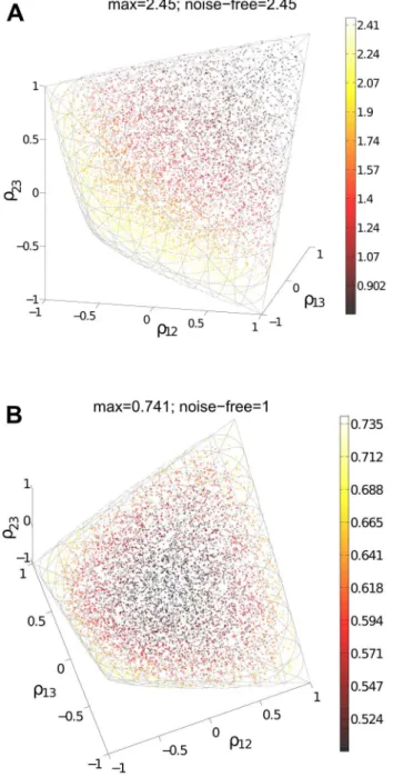
For a population ofN neurons, there areN(N{1)=2possible correlations to consider; naturally, as N increases, the optimal structure of noise correlations can therefore become more complex. Thus we illustrate the Theorem above with an example of 3 neurons encoding a scalar stimulus, in which there are 3 noise correlations to vary. In Fig. 3, we demonstrate two different cases, each with distinct (Cm)
ij~cov(mi,mj) matrix and vector Li~cov(s,mi)(values are given in Methods Section ‘‘S:numerics’’).
In the first case, there is a unique optimum (panel A, largest information is associated with the lightest color). In the second case, there are 4 disjoint optima (panelB), all of which lie on the boundary of the spectrahedron.
In the next section, we will build from this example to a more complex one including more neurons. This will suggest further principles that govern the role of noise correlations in population coding.
Heterogeneously tuned neural populations
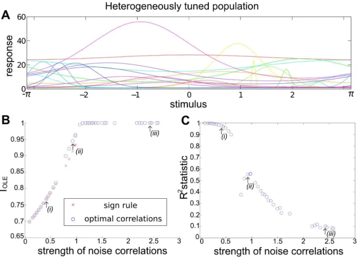
We next follow [8,9,15] and study a numerical example of a larger (N~20) heterogeneously tuned neural population. The stimulus encoded is the direction of motion, which is described by a 2-D vector~ss~(cos(h),sin(h))T. We used the same parameters
numerical examples and simulation’’. The tuning curve for each neuron was allowed to have randomly chosen width and magnitude, and the trial-to-trial variability was assumed to be Poisson: the variance is equal to the mean. As shown in Fig. 4A, under our choice of parameters the neural tuning curves – and by extension, their responses to the stimuli – are highly heterogenous. Once again, we quantify coding byIOLE(see definition in Section
‘‘Problem setup’’ or Eq. (12) in Methods).
Our goal with this example is to illustrate two distinct regimes, with different properties of the noise correlations that lead to optimal coding. In the first regime, which occurs closest to the case of independent noise, the SR determines the optimal correlation structure. In the second, moving further away from the independent case, the optimal correlations may disobey the SR. (A related effect was found by [8]; we return to this in the Discussion.) We accomplish this in a very direct way: for gradually increasing the (additional) constraint on the Euclidean norm of correlations (Eq. (18) in Methods Section ‘‘Defining the informa-tion quantities, signal and noise correlainforma-tions’’), we numerically search for optimal noise correlation matrices and compare them to predictions from the SR.
In Fig. 4 B we show the results, comparing the information attained with noise correlations that obey the sign rule with those that are optimized, for a variety of different noise correlation strengths. As they must be, the optimized correlations always produce information values as high as, or higher than, the values obtained with the sign rule.
In the limit where the correlations are constrained to be small, the optimized correlations agree with the sign rule; an example of these ‘‘local’’ optimized correlations is shown in Fig. 5 ADG, corresponding to the point labeled (i) in Fig. 4 BC. This is predicted by Theorem 1. In this ‘‘local’’ region of near-zero noise correlations, we see a linear alignment of signal and noise correlations (Fig. 5D). As larger correlation strengths are reached (points(ii)and(iii)in Fig. 4BC), we observe a gradual violation of the sign rule for the optimized noise correlations. This is shown by the gradual loss of the linear relationship between signal and noise correlations in Fig. 4Dvs.Evs.F, as quantified by theR2statistic.
Interestingly, this can happen even when the correlation coefficients continue have reasonably small values, and are broadly consistent with the ranges of noise correlations seen in physiology experiments [3,8,24].
The two different regimes of optimized noise correlations arise because, at a certain correlation strength, the correlation strength can no longer be increased along the direction that defines the sign rule without leaving the region of positive semidefinite covariance matrices. However, correlation matrices still exist that allow for more informative coding with larger correlation strengths. This reflects the geometrical shape of the spectrahedron, wherein the optima may lie in the ‘‘corners’’, as shown in Fig. 3. For these larger-magnitude correlations, the sign rule no longer describes optimized correlations, as shown with an example of optimized correlations in Fig. 5CF.
Fig. 5 illustrates another interesting feature. There is a diverse set of correlation matrices, with different Euclidean norms beyond the value of (roughly) 1.2, that all achieve the same globally optimal information level. As we see in the next section, this
Figure 3. Optimal coding is obtained on the boundary of the allowed region of noise correlations.For fixed neuronal responses variances and tuning curves, we compute coding performance – quantified byIOLEinformation values – for different values of the
pair-wise noise correlations. To be physically realizable, the correlation coefficients must form a positive semi-definite matrix. This constraint defines a spectrahedron, or a swelled tetrahedron, for theN~3cells used. The colors of the points representIOLEinformation values. With
different parametersCmandL(see values in Methods Section ‘‘Details
for numerical examples and simulations’’), the optimal configuration can appear at different locations, either unique (A) or attained at multiple disjoint places (B), but always on the boundary of the spectrahedron. In both panels, plot titles give the maximum value of
IOLEattained over the allowed space of noise correlations, and the
value ofIOLEthat would obtained with the given tuning curves, and
perfectly deterministic neural responses. This provides an upper bound on the attainable IOLE (see text Section ‘‘Noise cancellation’’).
Interestingly, in panel (A), the noisy population achieves this upper bound on performance, but this is not the case in (B). Details of parameters used are in Methods Section ‘‘Details for numerical examples and simulations’’.
phenomenon is actually typical for large populations, and can be described precisely.
Noise cancellation
For certain choices of tuning curves and noise variances, including the examples in Fig. 3Aand Section ‘‘Heterogeneously tuned neural populations’’, we can tell precisely the value of the globally optimized information quantities — that is, the informa-tion levels obtained with optimal noise correlainforma-tions. For the OLE, this global optimum is the upper bound on IOLE. This is shown
formally in Lemma 8, but it simply translates to an intuitive lower bound of the OLE error, similar to the data processing inequality for mutual information. This bound states that the OLE error cannot be smaller than the OLE error when there is no noise in the responses, i.e. when the neurons produce a deterministic
response conditioned on the stimulus. This upper bound may — and often will (Theorem 5) — be achievable by populations of noisy neurons.
Let us first consider an extremely simple example. Consider the case of two neurons with identical tuning curves, so that their responses arexi~m(s)zni, whereniis the noise in the response of
neuron i[f1,2g, and m(s) is the same mean response under stimuluss. In this case, the ‘‘noise free’’ coding is whenn1~n2:0 on all trials, and the inference accuracy is determined by the shape of the tuning curve m(s) (whether or not it is invertible, for example). Now let us consider the case where the noise in the neurons’ responses is non-zero but perfectly anti correlated, so that n1~{n2 on all trials. We can then choose the read-out as (x1zx2)=2~m(s)to cancel the noise and achieve the same coding
accuracy as the ‘‘noise free’’ case.
Figure 4. Heterogeneous neural population and violations of the sign rule with increasing correlation strength.We consider signal encoding in a population of 20 neurons, each of which has a different dependence of its mean response on the stimulus (heterogeneous tuning curves shown inA). We optimize the coding performance of this population with respect to the noise correlations, under several different constraints on the magnitude of the allowed noise correlations. Panel (B) shows the resultant – optimal given the constraint – values of OLE informationIOLE,
with different noise correlation strengths (blue circles). The strength of correlations is quantified by the Euclidean norm (Eq. (18)). For comparison, the red crosses show information obtained for correlations that obey the sign rule (in particular, pointing along the gradient giving greatest information for weak correlations); this information is always less than or equal to the optimum, as it must be. Note that correlations that follow the sign rule fail to exist for large correlation strengths, as the defining vector points outside of the allowed region (spectrahedron) beyond a critical length (labeled (ii)). For correlation strengths beyond this point, distinct optimized noise correlations continue to exist; the information values they obtain eventually saturate at noise-free levels (see text), which is1for the example shown here. This occurs for a wide range of correlation strengths. Panel (C) shows how well these optimized noise correlations are predicted from the corresponding signal correlations (by the sign rule), as quantified by theR2
statistic (between 0 and 1, see Fig. 5). For small magnitudes of correlations, theR2values are high, but these decline when the noise correlations are
larger.
The preceding example shows that, at least in some cases, one can choose noise correlations in such a way that a linear decoder achieves ‘‘noise-free’’ performance. One is naturally left to wonder whether this observation applies more generally.
First, we state the conditions on the noise covariance matrices under which the noise-free coding performance is obtained. We will then identify the conditions on parameters of the problem, i.e. the tuning curves (or receptive fields) and noise variances, under which this condition can be satisfied. Recall that the OLE is based on a fixed (across stimuli) linear readout coefficient vector A defined in Eq. (9)
Theorem 3.A covariance matrixCnattains the noise-free bound for
OLE information (and hence is optimal), if and only if CnA~ Cn(Cm){1
L~0. Here L is the cross-covariance between the stimuli responses (Eq. (11)),Cmis the covariance of the mean response (Eq. (10)),
andAis the linear readout vector for OLE, which is the same as in the noise-free case — that is,A~(CnzCm){1L~(Cm){1L
— when the condition is satisfied.
We note that when the condition is satisfied, the conditional variance of the OLE is ATCnA~0. This indicates that all the
error comes from the bias, if we as usual write the mean square error (for scalar s) in two parts, E(^ss{s)2
~Efvar(^ssDs)gz var(Ef g^ssDs {s). The condition obtained here can also be interpreted as ‘‘signal/readout being orthogonal to the noise.’’ While this perspective gives useful intuition about the result, we find that other ideas are more useful for constructing proofs of this and other results. We discuss this issue more thoroughly in Section ‘‘The geometry of the covariance matrix’’.
In general, this condition may not be satisfied by some choices of pairwise correlations. The above theorem implies that, given the tuning curves, the issue of whether or not such ‘‘noise free’’ coding is achievable will be determined only by the relative magnitude, or heterogeneity, of the noise variances for each neuron – the diagonal entries ofCn. The following theorem outlines precisely
the conditions under which such ‘‘noise-free’’ coding performance is possible, a condition that can be easily checked for given parameters of a model system, or for experimental data.
Theorem 4. For scalar stimulus, let qi~ ffiffiffiffiffiffiffiffiffiffiffiffi A2
iCiin q
, i~1, ,N,
whereA~(Cm){1L is the readout vector for OLE in the noise-free case.
Noise correlations may be chosen so that coding performance matches that which could be achieved in the absence of noise if and only if
maxfqigƒ 1 2
XN
i~1
qi: ð1Þ
When ‘‘v’’ is satisfied, all optimal correlations attaining the maximum form
aN(N{3)
2 dimensional convex set on the boundary of the spectrahedron.
When ‘‘~’’ is attained, the dimension of that set isN0(N0z1)
2 , whereN0is
the number of zeros infqig.
We pause to make three observations about this Theorem. First, the set of optimal correlations, when it occurs, is high-dimensional. This bears out the notion that there are many different, highly diverse noise correlation structures that all give the same (optimal) level of the information metrics. Second, and more technically, we note that the (convex) set of optimal correlations is flat (contained in a hyperplane of its dimension), as viewed in the higher
dimensional spaceRN(N2{1). A third intriguing implication of the theorem is that when noise-cancellation is possible, all optimal correlations are connected, as the set is convex (any two points are
Figure 5. In our larger neural population, the sign rule governs optimal noise correlations only when these correlations are forced to be very small in magnitude; for stronger correlations, optimized noise correlations have a diverse structure.Here we investigate the structure of the optimized noise correlations obtained in Fig. 4; we do this for three examples with increasing correlation strength, indicated by the labels(i),(ii),(iii)in that figure. First (ABC) show scatter plots of the noise correlations of the neural pairs, as a function of their signal correlations (defined in Methods Section ‘‘Defining the information quantities, signal and noise correlations’’). For each example, we also show (DEF) a version of the scatter plot where the signal correlations have been rescaled in a manner discussed in Section ‘‘Parameters for Fig. 1, Fig. 2 and Fig. 3’’, that highlights the linear relationship (wherever it exists) between signal and noise correlations. In both sets of panels, we see the same key effect: the sign rule is violated as the (Euclidean) strength of noise correlations increases. In (ABC), this is seen by noting the quadrants where the dots are located: the sign rule predicts they should only be in the second and fourth quadrants. In (DEF), we quantify agreement with the sign rule by theR2 statistic. Finally, (GHI) display histograms of the noise
correlations; these are concentrated around 0, with low average values in each case.
connected by a linear segment that also in the set), and thus the case of disjoint optima as in Fig. 3 B will never happen when optimal coding achieves noise-free levels. Indeed, in Fig. 3B, the noise-free bound is not attained.
The high dimension of the convex set of noise-canceling correlations explains the diversity of optimal correlations seen in Fig. 4B(i.e., with different Euclidean norms). Such a property is nontrivial from a geometric point of view. One may conclude prematurely that the dimension result is obvious if one considers algebraically the number of free variables and constraints in the condition of Theorem 3. This argument would give the dimension of the resulting linear space. However, as shown in the proof, there is another nontrivial step to show that the linear space has some finite part that also satisfies the positive semidefinite constraint. Otherwise, many dimensions may shrink to zero in size, as happens at the corner of the spectrahedron, resulting in a small dimension.
The optimization problem can be thought of as finding the level set of information function associated with as large as possible value while still intersecting with the spectrahedron. The level sets are collections of all points where the information takes the same value. These form high dimensional surfaces, and contain each other, much as layers of an onion. Here these surfaces are also guaranteed to be convex as the information function itself is. Next, note from Fig. 3 that we have already seen that the spectrahedron has sharp corners. Combining this with our view of the level sets, one might guess that the set of optimal solutions — i.e. the intersection — should be very low dimensional. Such intuition is often used in mathematics and computer science, e.g. with regards to the sparsity promoting tendency of L1 optimization. The high dimensionality shown by our theorem therefore reflects a nontrivial relationship between the shape of the spectrahedron and the level sets of the information quantities.
Although our theorem only characterizes the abundance of the set ofexactoptimal noise correlations, it is not hard to imagine the same, if not more, abundance should also hold for correlations that approximately achieve the maximal information level. This is indeed what we see in numerical examples. For example, note the long, curved level-set curves in Fig. 2 near the boundaries of the allowed region. Along these lines lie many different noise correlation matrices that all achieve the same nearly-optimal values ofIOLE. The same is true of the many dots in Fig. 3Athat
all share a similar ‘‘bright’’ color corresponding to largeIOLE.
One may worry that the noise cancellation discussed above is rarely achievable, and thus somewhat spurious. The following theorem suggests that the opposite is true. In particular, it gives one simple condition under which the noise cancellation phenomenon, and resultant high-dimensional sets of optimal noise correlation matrices, will almost surely be possible in large neural populations.
Theorem 5.If the fqigdefined in Theorem 4 are independent and
identically distributed (i.i.d.) as a random variable X on ½0,?) with
0vEf gX v?, then the probability
P the inequality of Eq:ð ð Þ1 is satifiedÞ?
1,as N??:
ð2Þ
In actual populations, theqimight not be well described as i.i.d..
However, we believe that the conditions of the inequality of Eq.(1) are still likely to be satisfied, as the contrary seems to require one neuron with highly outlying tuning and noise variance value (a few comparable outliers won’t necessary violate the condition, as their
magnitudes will enter on the right hand side of the condition, thus the condition only breaks with a single ‘‘outlier of outliers’’).
Discussion
Summary
In this paper, we considered a general mathematical setup in which we investigated how coding performance changes as noise correlations are varied. Our setup made no assumptions about the shapes (or heterogeneity) of the neural tuning curves (or receptive fields), or the variances in the neural responses. Thus, our results – which we summarize below – provide general insights into the problem of population coding. These are as follows:
N
We proved that thesign rule— if signal and noise correlations have opposite signs, then the presence of noise correlations will improve encoded information vs. the independent case — holds for any neural population. In particular, we showed that this holds for three different metrics of encoded information, and for arbitrary tuning curves and levels of heterogeneity. Furthermore, we showed that, in the limit of weak correlations, the sign rule predicts the optimal structure of noise correlations for improving encoded information.N
However, as also found in the literature (see below), the sign rule is not a necessary condition for good coding performance to be obtained. We observed that there will typically be a diverse family of correlation matrices that yield good coding performance, and these will often violate the sign rule.N
There is significantly more structure to the relationship between noise correlations and encoded information than that given by the sign rule alone. The information metrics we considered are allconvexfunctions with respect to the entries in the noise correlation matrix. Thus, we proved that the optimal correlation structures must lie on boundaries of any allowed set. These boundaries could come from mathematical constraints – all covariance matrices must be positive semidefinite – or mechanistic/biophysical ones.N
Moreover, boundaries containing optimal noise correlations have several important properties. First, they typically contain correlation matrices that lead to the same high coding fidelity that one could obtain in the absence of noise. Second, when this occurs there is a high-dimensional set of different correlation matrices that all yield the same high coding fidelity – and many of these matrices strongly violate the sign rule.N
Finally, for reasonably large neural populations, we showed that both the noise-free, and more general SR-violating optimal, correlation structures emerge while the average noise correlations remain quite low — with values comparable to some reports in the experimental literature.Convexity of information measures
Convexity of information with respect to noise correlations arises conceptually throughout the paper, and specifically in Theorem 2. We have shown that such convexity holds for all three particular measures of information studied above (IF,lin,IOLE, and Imut,G). Here, we show that these observations may reflect a
property intrinsic to the concept of information, so that our results could apply more generally.
distribution given by a nonnegative linear combination of the two, ~zzD~ss*p(~zzD~ss)~ap1(~zzD~ss)z(1{a)p2(~zzD~ss), a[½0,1. The mutual infor-mation must satisfy I(~zz,~ss)ƒaI(~xx,~ss)z(1{a)I(~yy,~ss). Notably, this fact can be proved using only the axiomatic properties of mutual information (the chain rule for conditional information and nonnegativity) [25].
It is easy to see how this convexity in conditional distributions is related to the convexity in noise correlations we use. To do this, we further assume that the two conditional means are the same,
Ef~xxD~ssg~Ef g~yyD~ss , and let ~xx,~yy be random vectors. Introduce an auxiliary Bernoulli random variableTthat is independent of~ss, with probability a of being 1. The variable~zz can then be explicitly constructed usingT: for any~ss, draw~zzaccording top1(~zzD~ss)ifT~1
and according top2(~zzD~ss)otherwise. Using the law of total covariance, the covariance (conditioned on~ss) between thei,jelements of~zzis
cov~ss(zi,zj)~E cov~ss(zi,zjDT)
zcov~ss(E~ssfziDTg,E~ssfzjDTg)
~acov~ss(zi,zjDT~1)z(1{a)cov~ss(zi,zjDT~0)z0
~acov~ss(xi,xj)z(1{a)cov~ss(yi,yj):
This shows that the noise covariances are expressed accordingly as linear combinations. If the information depends only on covariances (besides the fixed means), as for the three measures we consider, the two notions of convexity become equivalent. A direct corollary of this argument is that the convexity result of Theorem 2 also holds in the case of mutual information for conditionally Gaussian distributions (i.e., such that~xxgiven~ssis Gaussian distributed).
Sensitivity and robustness of the impact of correlations on encoded information
One obvious concern about our results, especially those related to the ‘‘noise-free’’ coding performance, is that this performance may not be robust to small perturbations in the covariance matrix – and thus, for example, real biological systems might be unable to exploit noise correlations in signal coding. This issue was recently highlighted, in particular, by [26].
At first, concerns about robustness might appear to be alleviated by our observation that there is typically a large set of possible correlation structures that all yield similar (optimal) coding performance (Theorem 4). However, if the correlation matrix was perturbed along a direction orthogonal to the level set of the information quantity at hand, this could still lead to arbitrary changes in information. To address this matter directly, we explicitly calculated the following upper bound for the sensitivity of information, orcondition numberkwith respect (sufficiently small) perturbations. The condition numberk is defined as the ratio of relative change in the function to that in its variables. For example, the condition number corresponding to perturbing Cn is the
smallest number kF,lin:Cn that satisfies
DDIF,linD DIF,linD
ƒkF,lin:Cn
EDCnE ECnE.
Similarly one can define condition numberkF,lin:+mfor perturbing
the tuning of neurons+m.
Proposition 6. The local condition number of IF,lin under
perturbations ofCn(where magnitude is quantified by 2-norm) is bounded by
kF,lin:Cnƒ2k2(Cn):~2E(Cn)
{1E
2:ECnE2~ 2lmax
lmin , ð3Þ
where lmax and lmin are the largest and smallest eigenvalue of Cn
respectively. Herek2is the condition number with respect to the 2-norm, as defined in the above equation.
Similarly, the condition number for perturbing of+mis bounded by
kF,lin:+mƒ3
ffiffiffiffiffiffiffiffiffiffiffiffiffiffiffiffiffiffi k2(Cn)K
p maxiE(+m):,iE2
miniE(+m):,iE2, ð4Þ
where(+m):,iis thei-th column of+mand assume(+m):,i=0for alli. Here Kis the dimension of the stimuluss.
Though stated for IF,lin, same results also hold forIOLE when
replacingCn by CmzCn in Eq. (3) and (4). We believe that a
similar property is possible to derive for mutual informationImut,G,
but that the expression could be quite cumbersome; we do not pursue this further here.
To interpret this Proposition, we make the following observa-tions which explain when the sensitivity or condition numbers will (or will not) be themselves reasonable in size, for given noise correlationsCn. In our setup, the diagonal ofCn(orCmzCnfor
OLE) is fixed, and thereforelmax is bounded (Gershgorin circle theorem). As long asCn(orCmzCn) is not close to singular, the
information should therefore be robust, i.e. with a reasonably bounded condition number. For OLE, asCmzCn Cm, we always
have a universal bound ofkdetermined only byCm. For the linear
Fisher information, however, nearly singular Cn can more
typically occur near optimal solutions; in these cases, the condition numbers will be very large.
Relationship to previous work
Much prior work has investigated the relationship between noise correlations and the fidelity of signal coding [3,5–11,13–16]. Two aspects of our current work complement and generalize those studies.
The first are our results on the sign rule (Section ‘‘The sign rule revisited’’). Here, we find that, if each cell pair has noise correlations that have the opposite sign vs. their signal correlations, the encoded information is always improved, and that, at least in the case of weak noise correlations, noise correlations that have the same sign as the signal correlations will diminish encoded information. This effect was observed by [6] for neural populations with identically tuned cells. Since the tuning was identical in their work, all signal correlations were positive. Thus, their observation that positive noise correlations diminish encoded information is consistent with the SR results described above.
Relaxing the assumption of identical tuning, several studies followed [6] that used cell populations with tuning that differed from cell to cell, but maintained some homogeneous structure – i.e., identically shaped, and evenly spaced (along the stimulus axis) tuning curves, e.g., [5,7]. The models that were investigated then assumed that the noise correlation between each cell pair was a decaying function of the displacement between the cells’ tuning curve peaks. The amplitude of the correlation function – which determines the maximal correlation over all cell pairs, attained for ‘‘nearby’’ cells – was the independent variable in the numerical experiments. Recall that these nearby (in tuning-curve space) cells, with overlapping tuning curves, will have positive signal correla-tions. These authors found that positive signs of noise correlations diminished encoded information, while negative noise correlations enhanced it. This is once again broadly consistent with the sign rule, at least for nearby cells which have the strongest correlation. Finally, we note that [5,10,12] give a crisp geometrical interpre-tation of the sign rule in the case ofN~2cells.
[3,6,19], which is certainly not in keeping with the sign rule. This underscores the need for new theoretical insights. To this effect, we demonstrated that, while noise correlations that obey the sign rule are guaranteed to improve encoded information relative to the independent case, this improvement can also occur for a diverse range of correlation structures that violate it. (Recall the asymmetry of our findings for the sign rule: noise correlations that violate the sign rule are only guaranteed to diminish encoded information if those noise correlations are very weak).
This finding is anticipated by the work of [8,9,14], who used elegant analytical and numerical studies to reveal improvements in coding performance in cases where the sign rule was violated. They studied heterogeneous neural populations, with, for exam-ple, different maximal firing rates for different neurons. In particular, these authors show how heterogeneity can simulta-neously improve the accuracy and capacity of stimulus encoding [14], or can create coding subspaces that are nearly orthogonal to directions of noise covariance [8,9]. Taken together, these studies show that the same noise correlation structure discussed above – with nearby cells correlated – could lead to improved population coding, so long as the noise correlations are sufficiently strong. [8] also demonstrated that the magnitude of correlations needed to satisfy the ‘‘sufficiently strong’’ condition decreases as the population size increases, and that in the large N limit, certain coding properties become invariant to the structure of noise correlations. Overall, these findings agree with our observations about a large diversity of SR-violating noise correlation structures that improve encoded information.
One final study requires its own discussion. Whereas the current study (and those discussed above) investigated how coding relates to noise correlations with no concerns for the biophysical origin of those correlations [17], studied a semi-mechanistic model in which noise correlations were generated by inter-neuronal coupling. They observed that coupling that generates anti-SR correlations is beneficial for population coding when the noise level is very high, but that at low noise levels, the optimal population would follow the SR. Understanding why different mechanistic models can display different trends in their noise correlations is important, and we are currently investigating that issue.
The geometry of the covariance matrix
One geometrical, and intuitively helpful, way to think about problems involving noise correlations is to ask when the noise is ‘‘orthogonal to the signal’’: in these cases, the noise can be separated from or be orthogonal to the signal, and high coding performance is obtained. This geometrical view is equally valid for the cases we study (e.g., the conditions we derive in Theorem 3), and is implicit in the diagrams in Figure 1. To make the approach explicit, one could perform an eigenvector analysis on the covariance matrices at hand, where quantities like linear Fisher information are rewritten as a sum of projections of the tuning vector to the eigen-basis of the covariance matrix, weighted by the appropriate eigenvalues.
This invites the question of whether a simpler way to obtain the results in our paper wouldn’t be to consider how covariance eigenvectors and eigenvalues could be manipulated more directly. For example, if one could simply ‘‘rotate’’ the eigenvectors of the covariance matrix out of the signal direction – or shrink the eigenvalues in that direction – one would necessarily improve coding performance. So why don’t we simply do this when exploring spaces of covariance matrices? The reason is that these eigenvalue and eigenvector manipulations are not as easy to enact as they might at first sound (to us, and possibly to the reader). Recall that we asked how noise correlations affect coding subject to the specific constraint that the noise variance of each neuron is
fixed, which translates in general to rather complex constraints on the eigenvalues and eigenvectors. For example, the eigenvalues of a fixed-diagonal covariance matrix cannot beequivalentlydescribed by simply having a fixed sum (which is a necessary condition for the diagonals to be constant, but is not a sufficient one). These facts limit the insights that a direct approach to adjusting eigenvalues and eigenvectors can have for our problem, and emphasize the non-trivial nature of our results.
An exception comes, for example, in special cases when the covariance matrix has a circulant structure, and consequently always has the Fourier basis for eigenvectors. These cases include many situations considered in the literature [8,10]. For contrast, the covariance matrices we studied were allowed to change freely, as long as the diagonals remained fixed.
Limitations and extensions
We have developed a rich picture of how correlated noise impacts population coding. For our results on noise cancellation in particular, this was done by allowing noise correlations to be chosen from the largest mathematically possible space (i.e., the entire spectrahedron). This describes the fundamental structure of the problem at hand, but are conclusions derived in this way important for biology? It is not hard to imagine many biological constraints that may further limit the range of possible noise correlations (e.g., limits on the strength of recurrent connections or shared inputs). On the one hand, the likelihood that the underlying phenomena could be found in biological systems seems increased by the fact that many different correlation matrices will suffice for noise free coding and that, as we discuss in Proposition 6, information levels appear to have some robustness under perturbations of the underlying correlation matrices.
However, care must still be taken in interpreting what we mean by ‘‘noise free.’’ As emphasized by, e.g., [8,27], noise upstream from the neural population in question can never be removed in subsequent processing. Therefore, the ‘‘noise free’’ bound we discuss in Lemma 8 should not allow for a higher information level than that determined by this upstream noise. In some cases, this fact could lead to a consistency requirement on either the set of signal correlationsCm, the set of allowed noise correlationsCn, or both. To
specify these constraints and avoid possible over-interpretations of the abstract coding model as we study, one could combine a explicit mechanistic model with the present approach.
On another note, we have asked what noise correlations allow for linear decoders to best recover the stimulus from the set of neural population responses. At the same time, there is reason to be wary of linear decoders [28] (see also [16]), as they might miss significant information that is only accessible via a non-linear read-out. Furthermore, given the non-linearity inherent in dendritic processing and spike generation [29], there is added motivation to consider information without assuming linearity.
Furthermore, we have herein restricted ourselves to asking about pairwise noise correlations, while there are many studies that identify higher-order correlations (HOC) in neural data [30,31], and some numerical results [32] that hint at when those HOC are beneficial for coding. In light of this study, it is interesting to ask whether we can derive a similarly general theory for HOC, and to investigate how the optimal pairwise and higher-order correlations interrelate. Note this issue is closely related to the type of decoder that is assumed: the performance of linear decoder (as measured by mean squared error) depends on the pairwise correlations, but not HOC. Therefore the effect of HOC must be studied in the context of nonlinear coding.
For generality, we made no assumptions on the structure of these statistics, and any links among them. This suggests two questions for future work: whether an arbitrary set of such statistics is realizable in a constructive model of random variables, and whether there are any typical relationships between these statistics when they arise from tuned neural populations. As a preliminary investigation, we partially confirmed the answer to the first question, except for a ‘‘zero measure’’ set of statistics, under generic assumptions (data not shown).
Experimental implications
Recall that we observed that, in general, for a given set of tuning curves and noise variances, there will be a diverse family of noise correlation matrices that will yield good (optimal, or near-optimal) performance. This effect can be observed in Figs. 2, 3, and 5, as well as our result about the dimension of the set of correlation matrices that yield (when it is possible) noise-free coding performance (Theorem 4).
At least compared with the alternative of a unique optimal noise correlation structure, our findings imply that it could be relatively ‘‘easy’’ for the biological system to find good correlation matrices. At the same time, since the set of good solutions is so large, we should not be surprised to see heterogeneity in the correlation structures exhibited by biological systems. Similar observations have previously been made in the context of neural oscillators: Prinz and colleagues [33] observed that neuronal circuits with a variety of different parameter values could produce the types of rhythmic activity patterns displayed by the crab stomatogastric ganglion. Consequent-ly, there is much animal-to-animal variability in this circuit [34], even though the system’s performance is strongly conserved.
At the same time, the potential diversity of solutions could present a serious challenge for analyzing data (cf. [26]). Notice, that, at least for theN~3cases of Figs. 2 and 3 for example, how much the performance can vary as one of the correlation coefficients is changed, while keeping the other ones fixed. If this phenomenon is general, it means that, in an experiment where we observe a (possibly small) subset of the correlation coefficients, it may be very hard to know how those correlations actually affect coding: the answer to that question depends strongly on all of the other (unobserved) correlation coefficients. As our recording technologies improve [35], and we make more use of optical methods, these ‘‘gaps’’ in our datasets will get smaller, and this issue may be resolved; further theoretical work to gauge the seriousness of the underlying issue is also needed. In the meanwhile, caution seems wise when analyzing noise correlations in sparsely sampled data.
Finally, recall that the optimal noise correlations will always lie on the boundary of the allowed region of such correlations. Importantly, what we mean by that boundary is flexible. It may be the mathematical requirement of positive semidefinite covariance matrices – the loosest possible requirement – or there may be tighter constraints that restrict the set of correlation coefficients. Since biophysical mechanisms determine noise correlations, we expect that there will be identifiable regions of possible correlation coefficients that are possible in a given circuit/system. Under-standing those ‘‘allowed’’ regions will, we anticipate, be important for attempts to relate noise correlations to coding performance, and ultimately to help untangle the relationship between structure and function in sensory systems.
Methods
In the Methods below, we will first revisit the problem set-up, and define our metrics of coding quality. We will then prove the
theorems from the main text. Finally, we will provide the details of our numerical examples. A summary of our most frequently used notation is listed in Table 1.
Summary of the problem set-up
We consider populations of neurons that encode a stimulus~ssby their noisy responsesxi. For simplicity, we will suppress the vector
notation in the Methods Unless otherwise stated, most of our results apply equally well to either scalar, or multi-dimensional, stimuli.
The mean activity or ‘‘tuning’’ of the neurons are described by
mi(s)~EfxiDsg. In the case of scalar stimuli, this corresponds to the
notion of a tuning curve. For more complex stimuli, this is more aligned with the idea of a receptive field.
The trial-to-trial noise part inxi, given a fixed stimulus, can be
described by the conditional covarianceCn
ij~cov xi,xjDs
(super-script n denotes ‘‘noise’’). In particularCn
ii~varðxiDsÞ are noise
variances of each neuron.
We ask questions of the following type: given fixed tuning curves
mand noise variancesCn
ii, how does the choice of noise covariance
structureCn
ij,i=jaffect linear Fisher informationIF,lin(see Section
‘‘Defining the information quantities, signal and noise correla-tions’’)?
Besides the local information measure IF,lin that quantifies
coding near a specific stimulus, we also considered global measures that describe overall coding of the entire ensemble of stimuli. These are IOLE and Imut,G, described in Section ‘‘Defining the
information quantities, signal and noise correlations’’. For these quantities, the relevant noise covariance is cov(xi,xj)~ E cov xi,xjDs
. We overload the notation withCn~cov(xi,xj)
in these global coding contexts. The optimization problem can then be identically stated forIOLEandImut,G.
Defining the information quantities, signal and noise correlations
Linear Fisher information. Linear Fisher information quantifies how accurately the stimulus near a value s can be decoded by a local linear unbiased estimator, and is given by
IF,lin~+mT(Cn)
{1+m:
ð5Þ
In the case of aKdimensional stimulus the same definition holds, with
+m~ Lm1 Ls1
Lm1 LsK
..
. ... ...
LmN Ls1
LmN LsK 0
B B B B B @
1
C C C C C A
: ð6Þ
In order for IF,lin to be defined by Eq. (5), we assume Cn is
invertible and hence positive definite:Cn]0. It can be shown that I{1
F,linis the (attainable) lower bound of the covariance matrix of the
error of any local linear unbiased estimator. Here the term lower bound is used in the sense of positive semidefiniteness, that is the ordering A B if and only if A{B 0. To obtain a scalar information quantity, we considertr(IF,lin)and also denote this by IF,linif not stated otherwise.