National Center of Experimental Mineralogy and Petrology, University of Allahabad, Utter Pradesh, India.
IPGP, Peris France.
Shyam S. Rai
National Geophysical Research Institute, Hyderabad, Andhra Pradesh.
Abstract
In the recent years, earthquakes have been used in understanding the Earth. The travel times of the body waves; P and S waves, the dispersion of the group and phase velocities of the surface waves and the information derived from the normal modes of the Earth gave information to extract the structure of the Earth’s interior.
I Introduction to Seismic Noise
The Earth itself involves a complex system of interactions between its climate, ocean and lithosphere which operate continuously. One of the results of these interactions is called the random seismic wavefield or seismic noise. There are various causes of seismic noise that leave different marks on the spectrum. The most energetic component is the oceanic microseisms which is a result of the interaction of atmosphere, ocean and the coast. Perturbations in the atmosphere due to strong storms impact on the ocean to set up standing wave patterns which create continuous pressure on the sea bottom, with variable intensity. The disturbance of the sea bottom results in the emergence of the elastic waves as for an earthquake or an explosion. The major difference is that the random wavefield has a chaotic nature in contrast to earthquakes or explosive generated elastic waves [1].
The standing waves in the ocean also send pressure waves with the atmosphere as microbaroms that can couple to the Earth to produce seismic signals. Although weaker than the microseisms, the microbaroms can provide local excitation. In recent years, the extraction of Greens function from the ambient noise field has emerged as an important tool to understand the Earth. The resultant waveform from the cross-correlation of random waves recorded at two different stations corresponds to the Greens function as if an impulsive force is applied at the one station and recorded at the other station [1][2].
For geophysics, it was first shown by Claerbout (1968) that the autocorrelation of the transmission response of the Earth corresponds to the superposition of the reflection response and its acausal counterparts. Recent work from Shapiro Campillo (2004); Shapiro et al. (2005) showed that by using two stations, it is possible to extract information along the connecting path by just using the Earths noise.
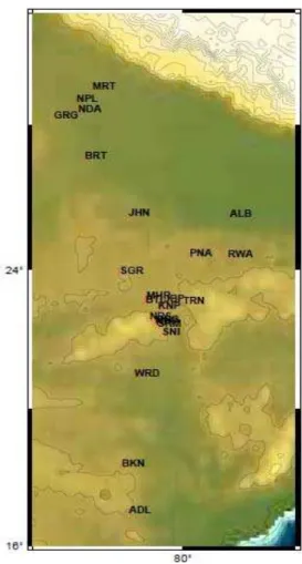
Figure 1 Location of Broadband seismic station installed in central India during 2005-2006 by NGRI, Hyderabad
II Broadband Location and Data Available
Table 1: Seismic station with sensor number and DAS number
III Measurement of Group Velocity
Figure 2: The time period versus group velocity contour plot of ALB station is shown. The group velocity for different period picked from contour in fundamental mode.
IV Data Processing Methodology
The ambient noise processing for the reconstructing the Green’s function of the medium between the path of connecting two stations primarily relies on simultaneous recordings. In addition to this, sufficiently long times of recording at the two stations will improve the reliability, and the signal to noise ratio of the estimates. We list the steps taken for the calculation of signal estimates of Greens function between two stations as[4]:
1. Prepare daily SAC files for each of the stations.
2. Remove the spurious days due to the instrument problem from seismic records.
3. Divide the full day record into 1 hour segments and compute the cross- correlations for the corresponding station pairs with 1 hour overlap and then average out the daily estimate.
4. Stack all of the averaged cross-correlations of the individual days to improve the signal . To noise ratio of the signal signal. In this procedure we do not attempt to exclude seismic [5]
IV.1 Single Station Data Preparation
The first phase of data processing consists of preparing waveform data for each station individually. The purpose of this stage to accenture broadband ambient noise source by attempting to remove earthquake signal and instrumental irregularities that leads to obscure ambient noise phase I of data processing: removal of instrumental response , de-meaning, de trending and bandpass filtering the seismogram, time domain normalization and spectral whitening [5]. This procedure is applied to single day of data. Day data with less than 80
IV.2 Temporal Normalization
Time domain normalization is a procedure for reducing the effect of cross correlation of earthquake, instrument irregularities and non stationary noise source near to station. Earthquake are among the most significant impediments to automated data processing. There are five different method to identify and remove the earthquake. We used automated event detection and removal in which 30 min of the waveform are set to zero if the amplitude of waveform is above the critical threshold [7].
IV.3 Spectral Normalization or whitening
Figures: 3 (a) Raw and (b) spectrally whitened amplitude spectra for 1 sample vertical data
IV.4 Cross Correlation, Stacking and Signal Emergence
After the preparation of the daily time-series [10], the next step in the data processing scheme (Phase2) is cross-correlation and stacking. Although some inter-station distances may be either too short or too long to obtain reliable measurements, we perform cross-correlations between all possible station pairs and perform data selection later. This yields a total of n(n -1)/2 possible station pairs, where n is the number of stations. Cross-correlation is performed daily in the frequency domain. After the daily cross-Cross-correlations are returned to the time domain they are added to one another, or stacked, to correspond to longer time series. Alternately, stacking can be done in the frequency domain which would save the inverse transform.
We prefer the organization that emerges from having daily raw time series and cross- correlations that are then stacked further into weekly, monthly, yearly, etc. time-series. In any event, the linearity of the cross-correlation procedure guarantees that this method will produce the same result as cross-cross-correlation applied to the longer time series. The resulting cross-correlations are two-sided time functions with both positive and negative time coordinates, i.e. both positive and negative correlation lags [10].
The time-series needed will depend on the group speeds of the waves and the longest inter station distance. The positive lag part of the cross-correlation is sometimes called the causal signal and the negative lag part the acausal signal. These waveforms represent waves traveling in opposite directions between the stations. Several examples of cross-correlations have been shown. some two-sided cross-correlations for different time-series lengths.
Fig. 4 (a): Cross correlation of station pair ALB-GRG and, (b) station pair ADL-BRT
Figure 5 : Cross correlation after applying different band pass filter
The constructive interference of the propagation from the sources along the surface to xAand xBis sufficient to
allow the construction of the Greens function between xAand xB . The most direct contributions come from the
vicinity of xAand xBsince the result is
independent of the configuration of the surface V . In the case where the surface V is far from the points of xA
and xB , the integral of rather subtle interference effects is needed to represent the Green’s function between
these points. The Greens function ˆG(xA, xB)
will include all scattering and multipath effects. Wapenaar & Fokkema (2006) showed the approximations to
ignore the effects from outside the V in appropriate circumstances. If the volume V extends further than the
twice the slowest propagation time between xAand xB, then the any energy returning from outside the surface
V will have a sufficiently long delay to have a little practical effect[12][13].
V Coefficient
This is most important parameter set in the multiple frequency techniques. We control the Relative width of filter by changing the parameter. For lower central frequency the bandwidth is narrower. Alpha appears in the numerator of exponent ratio in expression of filtering function so by setting lower , we find the broader filter. Due to uncertainty we can not set very high. It would make narrower filter, which would cause long unreal time signal and the resolution of the spectrogram would decrease. However, by setting very low we make very broad filter that will cause real signal in time domain but this signal would be competed by lot of frequencies. There is an optimal which will keep the resolution of at the best level. On the other hand, the optimal value may change the central frequency.
V.1 Recommendations for multiple filter analysis
Levshin recommended that the value of change with distance. The following choices may be adequate for the period range of 0 - 50 sec
Table II alpha with depth distance
1000 25 2000 50 4000 100 8000 200
(a) (b)
( c ), (d) & (e)
Figure:6 (a): ADL-JBP station pair inverted result (b) ALB-JBP sation pair inverted data. (c) ALD-MRT inverted data: (d)ALD-SNI station pair data.(e) ADL-R3 surface wave inverted data
Conclusion
between each pair of stations. Short-period surface-wave dispersion curves are estimated from the Green functions using frequency-time analysis paths connecting these stations. For the shorter period Rayleigh wave, which is most sensitive to shallow crustal structures no deeper than about 10 km. For the 15-s Rayleigh wave, which is sensitive mainly to the middle crust down to depths of about 20 km, These results establish that Rayleigh wave Green functions extracted by cross-correlating long sequences of ambient seismic noise, which are discarded as part of traditional seismic data processing, contain information about the structure of the shallow and middle crust.
The use of ambient seismic noise as the source of seismic observations addresses several shortcomings of traditional surface-wave methods. It may seem initially surprising that deterministic information about Earth’s crust can result from correlations of ambient seismic noise. Each of frequency components of the surface wave will sample with differing earth radius. In general the seismic velocity of earth increase radially downward so that the longer wavelength wave component which prorogate deeper, will propagate faster than shallower one. Dziewonski et al. (1980) develop a narrow MFT which operate in frequency time domain for estimating the group velocity.
The position of the peak of wave packet is calculated and divided by the source receiver distance to estimate the group velocity for that particular frequency. Figure 6.5 shows the cross correlation after applying different band pass filter. The compilation of data from 2005-2006 was done including all the broadband station across india for vertical component. Overall 276 individual cross correlation were calculated from the available data. The extracted two sided Green’s function of Rayleigh wave is observable for all the stations.
There is good spatial correspondence between features of group velocity and aspects of major geological provinces of India. The lower wave speeds have a strong correlation with thick sedimentary cover and petroleum deposit. Station GRG, NPL, NDA are very close and lying on same craton so they are grouped to Region R1, KHP, KNP, SNI are grouped to Region (R2), KHP, MNG, NRS are grouped to R3 region. We have 12 profile across the central part of India namely, ADL-BRT, ALB-JBP, ALB-MRT, ALB-R1, BRT-R3, GRG-R3, JHN-R1, JHN-GRG-R3, RWA-R1, TRN-R1, WRD-R3.We can compare group velocity in the station pairs for the time period of 10 sec(0.1Hz). These velocity show a high correlation with the major tectonic and geological features in the study area.
The high velocities are clear indicator of consolidated rock of Achaean and Proterozoic age in upper crust (Belousov et al.,1991). High velocity is possible indicator of volcanic rock in upper crust. The low velocity around 2.5Km/s due to thick sedimentary rock. Low velocity correlate with crustal temperature anomaly. For ALB-MRT group velocity is 2.94 Km/s, ALR-R3 group velocity is 3.28Km/s cab be explained as seismic station are located on proterozoic sediment basin. For ADL-BRT group velocity is 3.16 Km/s, ALB-JBP group velocity 2.87Km/s, ALB-SNI group velocity 2.33Km/s, BRT-R3 region, GRG-R3 region shows group velocity 3.41,3.49 respectively. For station pair Jhansi-R1, JHN-R3 group velocity is 2.33.For station pair RWA, TRN with R1 shows group velocity 2.26, 2.57 respectively.
For the Central Indian region, we have used to different velocity model during interpretation of the depth sampled by surface wave. In the first model uniform velocity 4.0K/s with depth was set in model. In second model varying velocity with depth was taken. The inversion result for both the models is similar.
Acknowledge
I would like to thanks Prof S. S. Rai, Scientist-G, National Geophysical Research Institute, Hyderabad for proving 24 seismic broadband data operated in Central India during 2005.