ACPD
10, 28471–28518, 2010Aerosol transport and transformation
with HSRL and WRF-Flexpart
B. de Foy et al.
Title Page
Abstract Introduction
Conclusions References
Tables Figures
◭ ◮
◭ ◮
Back Close
Full Screen / Esc
Printer-friendly Version Interactive Discussion
Discussion
P
a
per
|
Dis
cussion
P
a
per
|
Discussion
P
a
per
|
Discussio
n
P
a
per
|
Atmos. Chem. Phys. Discuss., 10, 28471–28518, 2010 www.atmos-chem-phys-discuss.net/10/28471/2010/ doi:10.5194/acpd-10-28471-2010
© Author(s) 2010. CC Attribution 3.0 License.
Atmospheric Chemistry and Physics Discussions
This discussion paper is/has been under review for the journal Atmospheric Chemistry and Physics (ACP). Please refer to the corresponding final paper in ACP if available.
Aerosol plume transport and
transformation in high spectral resolution
lidar measurements and WRF-Flexpart
simulations during the MILAGRO Field
Campaign
B. de Foy1, S. P. Burton2, R. A. Ferrare2, C. A. Hostetler2, J. W. Hair2, C. Wiedinmyer3, and L. T. Molina4,5
1
Department of Earth and Atmospheric Sciences, Saint Louis University, MO, USA
2
NASA Langley Research Center, Hampton, VA, USA
3
National Center of Atmospheric Research, Boulder, CO, USA
4
Molina Center for Energy and the Environment, CA, USA
5
ACPD
10, 28471–28518, 2010Aerosol transport and transformation
with HSRL and WRF-Flexpart
B. de Foy et al.
Title Page
Abstract Introduction
Conclusions References
Tables Figures
◭ ◮
◭ ◮
Back Close
Full Screen / Esc
Printer-friendly Version Interactive Discussion
Discussion
P
a
per
|
Dis
cussion
P
a
per
|
Discussion
P
a
per
|
Discussio
n
P
a
per
|
Received: 5 October 2010 – Accepted: 17 November 2010 – Published: 19 November 2010 Correspondence to: B. de Foy ([email protected])
ACPD
10, 28471–28518, 2010Aerosol transport and transformation
with HSRL and WRF-Flexpart
B. de Foy et al.
Title Page
Abstract Introduction
Conclusions References
Tables Figures
◭ ◮
◭ ◮
Back Close
Full Screen / Esc
Printer-friendly Version Interactive Discussion
Discussion
P
a
per
|
Dis
cussion
P
a
per
|
Discussion
P
a
per
|
Discussio
n
P
a
per
|
Abstract
The Mexico City Metropolitan Area (MCMA) experiences high loadings of atmospheric aerosols from anthropogenic sources, biomass burning and wind-blown dust. This pa-per uses a combination of measurements and numerical simulations to identify different plumes affecting the basin and to characterize transformation inside the plumes. The 5
airborne High Spectral Resolution Lidar measures extinction coefficients and extinction to backscatter ratio at 532 nm, and backscatter coefficients and depolarization ratios at 532 and 1064 nm. These can be used to identify aerosol types. The measurement cur-tains are compared with particle trajectory simulations using WRF-Flexpart for different source groups. The good correspondence between measurements and simulations 10
suggests that the aerosol transport is sufficiently well characterized by the models to estimate aerosol types and ages. Plumes in the basin undergo complex transport, and are frequently mixed together. Urban aerosols are readily identifiable by their low depolarization ratios and high lidar ratios, and dust by the opposite properties. Fresh biomass burning plumes have very low depolarization ratios which increase rapidly 15
with age. This rapid transformation is consistent with the presence of atmospheric tar balls in the fresh plumes.
1 Introduction
With maximum hourly concentrations above 300 µg/m3 for PM2.5 and above 600 µg/m3 for PM10 during the MILAGRO field campaign, aerosol concentrations are
20
a health concern in the Mexico City Metropolitan Area (MCMA) (Molina and Molina, 2002), (de Foy et al., 2008). These aerosols are the result of emissions from very dif-ferent sources including urban emissions, biomass burning smoke and wind suspen-sion of dust (Salcedo et al., 2006; Raga et al., 2001). The aerosol plumes are trans-ported by complex wind patterns in the basin leading to inhomogeneous plume dis-25
ACPD
10, 28471–28518, 2010Aerosol transport and transformation
with HSRL and WRF-Flexpart
B. de Foy et al.
Title Page
Abstract Introduction
Conclusions References
Tables Figures
◭ ◮
◭ ◮
Back Close
Full Screen / Esc
Printer-friendly Version Interactive Discussion
Discussion
P
a
per
|
Dis
cussion
P
a
per
|
Discussion
P
a
per
|
Discussio
n
P
a
per
|
(Jazcilevich et al., 2005; de Foy et al., 2006a. Intense vertical mixing in the afternoon leads to rapid venting of the urban plume outside of the basin (de Foy et al., 2006c). This paper focuses on identifying aerosol plumes in the MCMA basin during the MI-LAGRO field campaign using High Spectral Resolution Lidar (HSRL) measurements (Hair et al., 2008) and WRF-Flexpart particle trajectory simulations of known sources 5
(de Foy et al., 2009b).
MILAGRO (Megacity Initiative: Local And Global Research Observations) was an international field campaign in March 2006 that brought together hundreds of scientists. The goal was to study processes affecting atmospheric chemistry from the urban to the regional scale using the MCMA as a case study (Molina et al., 2010). Nested 10
within this field campaign was MCMA-2006 studying urban emissions and pollution within the basin, MAX-MEX studying aerosol transport and transformation in the urban plume leaving the basin, MIRAGE-Mex studying the pollution on the regional scale and INTEX-B studying large-scale impacts of pollution export (Molina et al., 2010). The lidar measurements used in this study are part of MAX-MEX and INTEX-B, and the 15
focus of the study is on the MCMA basin.
1.1 Aerosol composition
Aerosol composition at ground level in the MCMA was found to consist of roughly one quarter dust, one quarter secondary inorganic aerosols and one half organic matter for PM10, with similar patterns for PM2.5(Querol et al., 2008). Transmission Electron
Micro-20
scope (TEM) analysis found that most particles were coated or consisted of aggregates (Adachi and Buseck, 2008). Over half of the particles consisted of soot (black carbon) coated with organic matter and sulfates. This is consistent with Aiken et al. (2009) who found that half of the aerosols consisted of Secondary Organic Aerosol (SOA) and that the rest were split between primary urban emissions and biomass burning 25
ACPD
10, 28471–28518, 2010Aerosol transport and transformation
with HSRL and WRF-Flexpart
B. de Foy et al.
Title Page
Abstract Introduction
Conclusions References
Tables Figures
◭ ◮
◭ ◮
Back Close
Full Screen / Esc
Printer-friendly Version Interactive Discussion
Discussion
P
a
per
|
Dis
cussion
P
a
per
|
Discussion
P
a
per
|
Discussio
n
P
a
per
|
On the regional scale, Yokelson et al. (2007) and Crounse et al. (2009) found that biomass burning emissions could cause more than half of the organic aerosol mass in the plumes sampled by aircraft outside the basin and at higher altitudes. In addition, Christian et al. (2010) identified significant aerosol sources due to biofuel use and garbage burning throughout the region. These regional sources led to surface impacts 5
in the MCMA, although they remained smaller than the impacts from local sources (Aiken et al., 2010).
1.2 Aerosol transformation
The picture that arises of aerosols in the MCMA plume is one of a complex mixture of aerosols from very different sources. In addition, the plume is highly reactive and leads 10
to considerable formation of SOA. As the plume oxidizes, both the physical and optical properties evolve over a short time scale in a way that can be accounted for using bulk aerosol categories rather than detailed chemical composition (Jimenez et al., 2009). For the MCMA, rapid SOA formation was measured during the first day of plume trans-port. After that, total amounts of SOA did not increase even though oxidation continued 15
transforming the plume (DeCarlo et al., 2010). For plumes with high biomass burning content it was further shown that aging and transformation could add nearly half of the equivalent mass of the original primary organic aerosol (DeCarlo et al., 2010).
A detailed chemical analysis on the level of individual particles confirms the impor-tance of SOA by identifying that the most prevalent aerosol type contains mixed inor-20
ganic species coated in organic material (Moffet et al., 2010). Furthermore, the fraction of organic material increases with transport away from the MCMA. Fresh aerosols from the MCMA were found to have lower specific absorption which increased with distance travelled (Doran et al., 2007), although the relationship was weak and aerosol coating took place during the day but not at night (Doran et al., 2008). Similar results from 25
ACPD
10, 28471–28518, 2010Aerosol transport and transformation
with HSRL and WRF-Flexpart
B. de Foy et al.
Title Page
Abstract Introduction
Conclusions References
Tables Figures
◭ ◮
◭ ◮
Back Close
Full Screen / Esc
Printer-friendly Version Interactive Discussion
Discussion
P
a
per
|
Dis
cussion
P
a
per
|
Discussion
P
a
per
|
Discussio
n
P
a
per
|
but rather from an increase in the number of particles in the accumulation mode (Klein-man et al., 2009). This was found to correspond to an increase in particles in the ultra-fine and Aitken mode with photochemical age.
Studies of biomass burning plumes not limited to MILAGRO have found that they have a large range of optical properties depending on the type of fire and the age of the 5
plume (Reid et al., 2005). Janh ¨all et al. (2010) analyzed the geometric mean diameter and geometric standard deviation for fresh (less than 1 h old) and aged smoke and found that the fresh smoke had much smaller particles with a larger distribution of sizes. These small particles in the nucleation mode transfer to the accumulation mode within half an hour, but Janh ¨all et al. (2010) suggest that they have little influence on 10
optical properties.
Yokelson et al. (2009) identified tar balls during MILAGRO using TEM in plume sam-ples 10 to 30 min old, but not in the fresh sample that was collected within a few minutes of emissions. Atmospheric tar balls, not to be confused with blobs of oil in the ocean, are spherical particles that likely form within minutes from gas-to-particle conversion 15
in the plume, and are particularly abundant in the initial hours of transformation (Pos-fai et al., 2004). They typically have diameters between 30 and 500 nm and consist mainly of carbon and oxygen. They efficiently scatter and absorb light which makes them important in terms of regional haze and climate forcing (Hand et al., 2005). There is conflicting evidence of hygroscopicity, but it seems that aging and oxidation leads 20
to particle coating and enhanced solubility (Semeniuk et al., 2007). They have been called “brown carbon” because of their complex refractive indices and, in addition to young biomass burning plumes, have also been found in East-Asian outflow air masses (Alexander et al., 2008; Posfai and Buseck, 2010). Laboratory studies have further ex-amined their morphology (Chakrabarty et al., 2006) and suggest that they may have a 25
ACPD
10, 28471–28518, 2010Aerosol transport and transformation
with HSRL and WRF-Flexpart
B. de Foy et al.
Title Page
Abstract Introduction
Conclusions References
Tables Figures
◭ ◮
◭ ◮
Back Close
Full Screen / Esc
Printer-friendly Version Interactive Discussion
Discussion
P
a
per
|
Dis
cussion
P
a
per
|
Discussion
P
a
per
|
Discussio
n
P
a
per
|
1.3 Plume transport
Fast et al. (2007) describes the general meteorological conditions during MILAGRO along with the measurements available. Wind patterns were found to be represen-tative of the climatological average for Mexico City (de Foy et al., 2008) and include similar transport scenarios to the previous campaign, MCMA-2003 (de Foy et al., 5
2005), (Molina et al., 2007). The formation of convergence lines and very high mix-ing heights are important meteorological features in the basin that lead to rapid ventmix-ing of the plume and export into the free troposphere. During MILAGRO, maximum day-time boundary layer heights always reached 2000 m above ground level and frequently exceeded 4000 m (Shaw et al., 2007). SO2 was used as a tracer to identify verti-10
cal stratification of distinct plumes during the campaign (de Foy et al., 2009a). This showed that at night a low level industrial plume frequently led to high concentrations in the MCMA in combination with drainage flows around the basin slopes. The elevated plume from the Popocatepetl volcano, located on the southeastern edge of the basin, only mixed down to the surface under certain occasions during the day but otherwise 15
was transported aloft above the surface. This combination of daytime basin mixing and longer range transport stratified in the vertical can lead to a plug flow with segmented plumes travelling very rapidly at high altitude but much slower nearer the surface (Voss et al., 2010).
Lewandowski et al. (2010) performed an urban transect of the MCMA with a mobile 20
lidar. They observed directly the residual layers aloft, the mixed layer below growing during the day until it mixes with the residual layer, and the transport through the gap in the southeast of the basin. The valley to the south is at a lower elevation than the basin so that as the gap flow moves south, the MCMA plume continues at a constant height and is separated from the surface flow. The vertical stratification persists over 25
ACPD
10, 28471–28518, 2010Aerosol transport and transformation
with HSRL and WRF-Flexpart
B. de Foy et al.
Title Page
Abstract Introduction
Conclusions References
Tables Figures
◭ ◮
◭ ◮
Back Close
Full Screen / Esc
Printer-friendly Version Interactive Discussion
Discussion
P
a
per
|
Dis
cussion
P
a
per
|
Discussion
P
a
per
|
Discussio
n
P
a
per
|
The NASA Langley airborne HSRL acquired detailed high resolution profiles of aerosol extinction, optical depth, backscatter and depolarization during MILAGRO. The measurements are described in Sect. 2 and the Lagrangian particle simulations in Sect. 3. Simulations of urban, biomass burning and dust source types enables the identification of individual plumes in the data as well as an estimation of their ages. 5
Sect. 4 presents the results for biomass burning plumes and dust plumes, and then for urban transects in the MCMA and for flights following the plume as it is transported outside the basin. Sect. 5 discusses the relevance of the results to aerosol transport and transformation as well as for the evaluation of numerical simulations.
2 High spectral resolution lidar
10
The High Spectral Resolution Lidar technique was developed to separate the aerosol backscatter from molecular backscatter and therefore estimate aerosol extinction and backscatter coefficients independently (Shipley et al., 1983). This enables the di-rect measurement of the lidar ratio, which is the ratio of extinction to backscatter and provides an additional parameter for discriminating among aerosol types (Hair et al., 15
2008). The HSRL has been used to evaluate combined active and passive aerosol extinction profiles from satellite, and is being developed for space observation (Burton et al., 2010).
The National Aeronautics and Space Administration (NASA) Langley Research Cen-ter (LaRC) airborne High Spectral Resolution Lidar (HSRL) used during MILAGRO is 20
described in detail in Hair et al. (2008). The lidar uses a pulsed Nd:YAG laser with out-put at 532 nm and 1064 nm. An iodine vapor filter is used to discriminate between the Mie scattering of the aerosols and the Cabannes-Brillouin molecular scattering at the 532 nm wavelength. This provides independent measurements of aerosol backscat-ter and extinction coefficients. At 1064 nm, the standard backscatter lidar technique 25
ACPD
10, 28471–28518, 2010Aerosol transport and transformation
with HSRL and WRF-Flexpart
B. de Foy et al.
Title Page
Abstract Introduction
Conclusions References
Tables Figures
◭ ◮
◭ ◮
Back Close
Full Screen / Esc
Printer-friendly Version Interactive Discussion
Discussion
P
a
per
|
Dis
cussion
P
a
per
|
Discussion
P
a
per
|
Discussio
n
P
a
per
|
channels is performed internally thereby eliminating the need to calibrate against at-mospheric targets for which the aerosol loading is uncertain. The 1064 nm backscatter retrieval does rely on calibration to a region of low aerosol loading in the profile, but ben-efits from an estimate of the aerosol backscatter from the internally calibrated 532 nm channels.
5
Rogers et al. (2009) describe the evaluation of the HSRL during MILAGRO. The aerosol measurements were compared with in situ aerosol scattering and absorption measurements on board the C-130, G-1 and J-31 aircraft as well as ground based measurements from the Aerosol Robotic Network (AERONET). Bias in extinction coef-ficients at 532 nm were found to be below 3%, and root mean square differences below 10
50%.
Four intensive parameters that depend only on the aerosol type and not on the con-centration can be calculated from the measurements: the lidar ratio, the aerosol depo-larization ratio at 532 nm and 1064 nm, and the backscatter coefficient color ratio. The latter is defined as the backscatter at 532 nm divided by the backscatter at 1064 nm. 15
For the analysis, instead of using two depolarization ratios, we use the aerosol de-polarization ratio at 532 nm and the dede-polarization color ratio defined as the aerosol depolarization ratio at 1064 nm divided by that at 532 nm.
The lidar ratio has vertical resolution of 300 m and temporal resolution of 1 min (corresponding to 6 km horizontal resolution) whereas the depolarization ratio and 20
backscatter coefficients have a vertical resolution of 60 m and temporal resolution of 10 seconds (corresponding to 1 km horizontal resolution).
The depolarization ratio discriminates between spherical and non-spherical particles. The lidar ratio helps identify pollution which tends to be more absorbing, and hence have a higher ratio (M ¨uller et al., 2007). The backscatter color ratio is inversely related 25
(Sug-ACPD
10, 28471–28518, 2010Aerosol transport and transformation
with HSRL and WRF-Flexpart
B. de Foy et al.
Title Page
Abstract Introduction
Conclusions References
Tables Figures
◭ ◮
◭ ◮
Back Close
Full Screen / Esc
Printer-friendly Version Interactive Discussion
Discussion
P
a
per
|
Dis
cussion
P
a
per
|
Discussion
P
a
per
|
Discussio
n
P
a
per
|
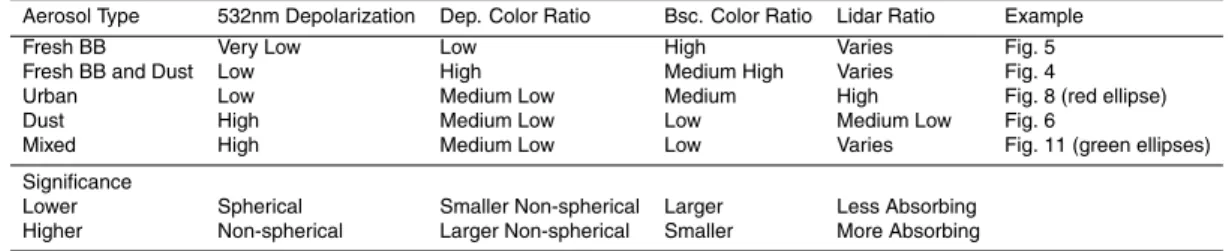
imoto and Lee, 2006; Ferrare et al., 2010). Table 1 provides an overview of the aerosol optical properties used in the discussion, along with information about different aerosol types and links to examples in the measurements.
Cattrall et al. (2005) used a clustering algorithm to classify aerosols into source types based on the intensive optical properties. This has been further developed to clas-5
sify aerosol types encountered during 10 field campaigns all over North America (Fer-rare et al., 2010). The HSRL typing analysis has been valuable for identifying smoke aerosols during the ARCTAS mission (Warneke et al., 2010) and urban aerosols during the MILAGRO mission (Molina et al., 2010).
The HSRL operated on 20 research flights during MILAGRO including the arriving 10
and departing flights. This paper focuses on the 10 flights between 3 March and 15 March. This period corresponds to the drier part of the campaign with fewer clouds, better data availability and more biomass burning and wind-blown dust.
3 Modeling
The meteorological simulations used in this study are described and evaluated in de-15
tail in de Foy et al. (2009b) and are the same as the ones used in the study of SO2
transport in the basin described in de Foy et al. (2009a). The model was evaluated by three different methods. First, statistical performance metrics were calculated using both surface observations and vertical profiles of temperature, humidity, wind speed and wind direction. Second, the model representation of wind clusters identified from 20
the data was compared for both surface wind patterns and radiosonde synoptic pat-terns. Third, the model was evaluated by comparing results from “Concentration Field Analysis”. This evaluates the model by seeing if trajectories based on the simulated wind fields are able to identify correctly known emissions of air pollutants based on surface measurements at different fixed sites.
25
ACPD
10, 28471–28518, 2010Aerosol transport and transformation
with HSRL and WRF-Flexpart
B. de Foy et al.
Title Page
Abstract Introduction
Conclusions References
Tables Figures
◭ ◮
◭ ◮
Back Close
Full Screen / Esc
Printer-friendly Version Interactive Discussion
Discussion
P
a
per
|
Dis
cussion
P
a
per
|
Discussion
P
a
per
|
Discussio
n
P
a
per
|
Forecast System (GFS) as initial and boundary conditions. There were three domains in the simulation with grid resolutions of 27, 9 and 3 km, 41 vertical levels and one-way nesting. Diffusion in coordinate space was used for domains 1 and 2, and in physical space for domain 3 (Z ¨angl et al., 2004). The following options were used: the Yonsei University (YSU) boundary layer scheme (Hong et al., 2006), the Kain-Fritsch 5
convective parametrization (Kain, 2004), the WSM6 microphysics scheme, the Dudhia shortwave scheme and the RRTM longwave scheme. High resolution satellite remote sensing was used to improve the land surface representation in the NOAH land surface model for domains 2 and 3 by using landuse, surface albedo, vegetation fraction and land surface temperature from the Moderate Resolution Imaging Spectroradiometer 10
(MODIS) as described in de Foy et al. (2006b).
Stochastic particle trajectories were calculated with FLEXPART (Stohl et al., 2005) using WRF-FLEXPART (Fast and Easter, 2006; Doran et al., 2008). Vertical diffusion coefficients were calculated based on the mixing heights and surface friction velocity from the mesoscale models. Sub-grid scale terrain effects were turned offand a re-15
flection boundary condition was used at the surface to eliminate all deposition effects. Particle locations were saved every hour for analysis.
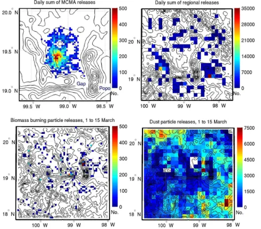
Separate particle simulations were carried out as tracers for urban MCMA emissions, urban emissions in the region surrounding the MCMA, biomass burning emissions and wind-blown dust emissions. Forward trajectories were calculated for every hour of the 20
field campaign with trajectories integrated for 48 h. Figure 1 shows the resulting grid of the daily sum of particle releases for each group. Figure 2 shows the hourly profile of the number of particles released for both the urban and the regional emissions used for each day, and the hourly variation of biomass burning and dust used for 1 to 15 March. For the urban plume, forward trajectories were calculated using urban CO emissions. 25
ACPD
10, 28471–28518, 2010Aerosol transport and transformation
with HSRL and WRF-Flexpart
B. de Foy et al.
Title Page
Abstract Introduction
Conclusions References
Tables Figures
◭ ◮
◭ ◮
Back Close
Full Screen / Esc
Printer-friendly Version Interactive Discussion
Discussion
P
a
per
|
Dis
cussion
P
a
per
|
Discussion
P
a
per
|
Discussio
n
P
a
per
|
vehicle counts and diurnal profiles (Lei et al., 2007). The grids were scaled to have a daily average of 2000 particles per hour released in the bottom 50 m of the boundary layer.
Anthropogenic emissions in the regions surrounding the MCMA were based on Mena-Carrasco et al. (2009) who used a number of sources. The bulk of the particles 5
released are due to the urban centers of Puebla to the east and Toluca to the west, with smaller contributions from Cuernavaca to the south and Pachuca to the northeast. For some of the plots and analysis, merged particle fields were created by scaling the regional emissions to the MCMA values and obtaining a single urban emissions field.
Tracers of biomass burning emissions were based on daily emission estimates of CO 10
calculated using the Fire INventory from NCAR (FINN) version 1, an emission frame-work method described in Wiedinmyer et al. (2006) and Wiedinmyer et al. (2010). Fire counts (MODIS Data Processing System) were provided by the University of Maryland, see MODIS Rapid Response project (2002) and Giglio et al. (2003). To account for the inconsistent daily coverage of the MODIS data in the tropical latitudes, fire detections 15
in these equatorial regions are counted for a 2-day period, following similar methods described by Al-Saadi et al. (2008). Land cover was determined with the MODIS Land Cover Type product (Friedl et al., 2010) and fuel loadings from Hoelzemann et al. (2004) and Akagi et al. (2010). Emission factors were taken from multiple sources (e.g., An-dreae and Merlet, 2001; M. O. AnAn-dreae, personal communications, 2008; Akagi et al., 20
2010).
The emissions are a revised version of the ones used in Aiken et al. (2010) and DeCarlo et al. (2010). Daily emissions totals are divided into hourly emissions starting at 8am of the current day until 8am the following day. This is to account for smoldering emissions that continue during the night, and for the fact that many of the fires are 25
ACPD
10, 28471–28518, 2010Aerosol transport and transformation
with HSRL and WRF-Flexpart
B. de Foy et al.
Title Page
Abstract Introduction
Conclusions References
Tables Figures
◭ ◮
◭ ◮
Back Close
Full Screen / Esc
Printer-friendly Version Interactive Discussion
Discussion
P
a
per
|
Dis
cussion
P
a
per
|
Discussion
P
a
per
|
Discussio
n
P
a
per
|
Tracers of dust emissions were calculated using the DUSTRAN dust transport mod-ule (Shaw et al., 2008) based on the WRF simulations. This parametrization is based on the friction velocity in the model and takes into account the land use type, soil type, vegetation fraction and soil moisture in estimating particulate mass loadings. We assumed medium-fine soils corresponding to clay-loam for the MCMA. Values of emis-5
sions in units of g/m2s were converted to number of particles with a proportionality constant, and emissions were grouped into a single area release for each two by two group of grid cells in order to reduce computational load. The focus of this paper is on the pattern of the emissions and the plume transport and so we shall not evaluate the quantities of dust emitted, but it is worth noting in passing that the DUSTRAN emis-10
sions are several orders of magnitude larger than the official MCMA inventory. Aerosol data suggests that the MCMA inventory is underestimated (Querol et al., 2008), and modeling studies suggest that the DUSTRAN emissions may be too high (Qian et al., 2010). Using an alternative model, Hodzic et al. (2009) found that wind-blown dust could account for 10% to 70% of PM2.5depending on meteorological conditions. The
15
estimates derived from DUSTRAN are consistent with this and suggest the ubiquitous presence of airborne dust in the region for the time period modeled.
An index of particle type was developed using the Flexpart simulations. For each emissions source, particles were counted inside grid cells corresponding to HSRL measurements. The cells were classified as being of a single aerosol type if that type 20
accounted for more than two thirds of the scaled particle count. They were classified as a mix of all three (urban, biomass burning and dust) if each type accounted for less than 40%. The particle fraction was obtained by scaling the number of particles from each source by the magnitude of the CO emissions. This was chosen because the CO inventory is relatively well constrained and has been found to provide good quantitative 25
ACPD
10, 28471–28518, 2010Aerosol transport and transformation
with HSRL and WRF-Flexpart
B. de Foy et al.
Title Page
Abstract Introduction
Conclusions References
Tables Figures
◭ ◮
◭ ◮
Back Close
Full Screen / Esc
Printer-friendly Version Interactive Discussion
Discussion
P
a
per
|
Dis
cussion
P
a
per
|
Discussion
P
a
per
|
Discussio
n
P
a
per
|
mass was similar to the biomass burning emissions, and from there use the same ratio of 10 to 1 for CO to PM2.5emissions. By adopting this method, we were able to identify areas that contained more urban or fire emissions than others, although it should be kept in mind that in practice, dust was present to some degree everywhere. The mean age of the particles was subsequently calculated based on the scaled particle counts. 5
4 Results
4.1 Biomass burning plumes
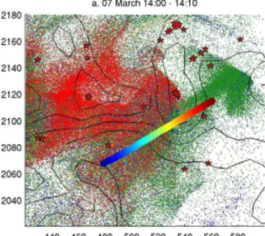
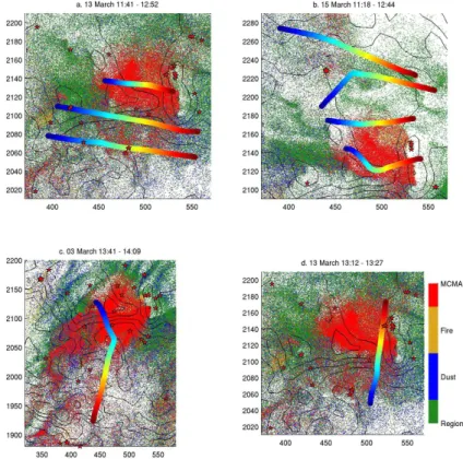
The HSRL measured numerous biomass burning plumes during the first half of the field campaign. Figure 3a and b show maps of two flight segments that sampled biomass burning plumes, with corresponding curtain plots shown in Figs. 4 and 5. These were 10
selected because the plumes have clear optical properties even though the simulations suffer from weak comparisons. Furthermore, they illustrate two contrasting types of optical properties. Twenty examples of biomass burning plumes sampled during the campaign are shown in the supplementary material, some of which are discussed in Sects. 4.3 and 4.4.
15
On 7 March the HSRL flew a leg south of the basin, moving northeastward towards the slopes of the Popocatepetl volcano as shown in Fig. 3a. The yellow ellipse on the left in Fig. 4 shows a smaller biomass burning plume in the valley to the south of the MCMA that is contained within the first 1000 m above ground level. The yellow ellipse to the right shows a bigger biomass burning plume on the eastern slope of the volcano, 20
that extends more than 2000 m above ground level. The green ellipse in the middle identifies a large plume of mixed aerosols south of the basin gap, between 3000 and 4500 mm.s.l..
The Flexpart simulations of biomass burning do not show many particles for the small plume on the left. However, Fig. 3a shows that there was a fire just northwest of 25
ACPD
10, 28471–28518, 2010Aerosol transport and transformation
with HSRL and WRF-Flexpart
B. de Foy et al.
Title Page
Abstract Introduction
Conclusions References
Tables Figures
◭ ◮
◭ ◮
Back Close
Full Screen / Esc
Printer-friendly Version Interactive Discussion
Discussion
P
a
per
|
Dis
cussion
P
a
per
|
Discussion
P
a
per
|
Discussio
n
P
a
per
|
in the simulations, barely seen as light blue on the navy background. The emissions model identified a small fire just south of the flight curtain (see Fig. 3a). In both cases, it is possible that the emissions estimates were too low for these fires and also that discrepancies in the transport direction were sufficient for the model to miss the bulk of the plume. In the middle of the figure, shown by the green ellipse, is a mixed plume 5
of dust, biomass burning and urban aerosols. This plume came from the MCMA basin through the mountain gap and was then transported as an elevated layer separated from the surface flow. In the simulations, the plume can be seen to be at the surface, below the green ellipse, because Flexpart transported it along terrain contours rather than at constant elevation. The separation of the flow passing over the basin rim will 10
be discussed further in Sect. 4.3.
The biggest difference in optical properties between the aerosols in the biomass burning plumes and the rest is the low aerosol depolarization ratio at 532 nm which is between 0.05 and 0.1, in contrast with regional values between 0.1 and 0.2. The high backscatter color ratio gives a clear signal of the plumes with values around 2 15
compared with 1 to 1.5 elsewhere. The high depolarization color ratio stands out more clearly for the bigger plume with values up to 2.5 compared to values from 1.5 to 2 for the background and the smaller plume. The lidar ratio is not very different from the surrounding areas, with values between 30 and 60.
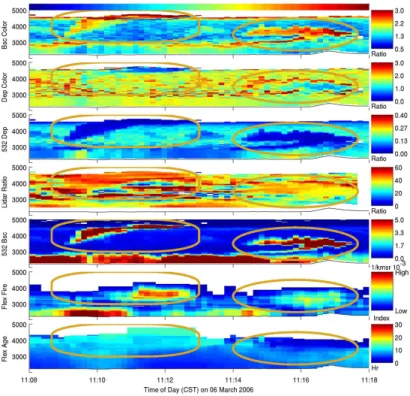
On 6 March, the HSRL performed a loop over the MCMA and detected an elevated 20
biomass burning plume transported above the surface urban layer. Fig. 3b shows the flight trajectory and the fire locations and Fig. 5 shows the curtain plots for this event. The yellow ellipses in the HSRL curtain plots highlight the two passes of the HSRL over the same plume. The Flexpart trajectories are in good agreement with the plumes showing that this is biomass burning smoke transported from a series of fires 25
ACPD
10, 28471–28518, 2010Aerosol transport and transformation
with HSRL and WRF-Flexpart
B. de Foy et al.
Title Page
Abstract Introduction
Conclusions References
Tables Figures
◭ ◮
◭ ◮
Back Close
Full Screen / Esc
Printer-friendly Version Interactive Discussion
Discussion
P
a
per
|
Dis
cussion
P
a
per
|
Discussion
P
a
per
|
Discussio
n
P
a
per
|
values up to 3 and the depolarization color ratio is lower with values below 1 for the higher parts of the plume. As will be seen below, the 6 March plume is indicative of a purer plume of biomass burning smoke with less dust content, and the plume on 7 March is indicative of a biomass burning plume with greater dust content.
4.2 Dust
5
Dust was ubiquitous during MILAGRO, especially during the first half of the campaign which was very dry (Fast et al., 2007). Figure 6 shows the largest dust plume in the data which was on the flanks of Pico de Orizaba, a dormant volcano 200 km to the east of the MCMA, as shown in Fig. 3c. The high backscatter coefficients can be seen to extend upwards to the top of the mixed layer. These are associated with some of the 10
highest values of aerosol depolarization ratios at 532 nm, in the range of 0.25 to 0.35. The depolarization color ratio is around 1, at the low end of measurements, and the backscatter color ratio is also low with values ranging from 0.4 to 0.6 (in contrast with values up to 3 for biomass burning plumes). The high aerosol depolarization ratios extend in a tail towards the west suggesting that there was some transport aloft, but 15
the low backscatter coefficients corresponding to this tail suggest that most of the dust has settled back to lower altitudes.
This transect is outside the fine domain for the WRF simulations. The model does simulate transport of emissions from the fine domain to the area, and it also simulates dust emissions using winds from the medium domain at a coarser resolution (9 km). 20
However, this resolution is too coarse to represent the localized feature and to create areas of intense emissions due to local flows. The model therefore does not capture this dust event even though it simulates the presence of dust in the region.
Further examples of dust plumes are presented in the supplementary material along with trajectory curtain plots. The optical properties are similar across the different 25
ACPD
10, 28471–28518, 2010Aerosol transport and transformation
with HSRL and WRF-Flexpart
B. de Foy et al.
Title Page
Abstract Introduction
Conclusions References
Tables Figures
◭ ◮
◭ ◮
Back Close
Full Screen / Esc
Printer-friendly Version Interactive Discussion
Discussion
P
a
per
|
Dis
cussion
P
a
per
|
Discussion
P
a
per
|
Discussio
n
P
a
per
|
4.3 Urban transects
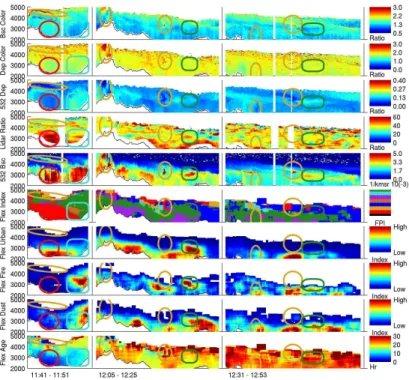
The HSRL performed transects of the MCMA basin during most of the flights. Fig-ures 7 a and b show maps of the flight segments over the MCMA, with the correspond-ing HSRL curtains shown in Fig. 8 for the three transects on 13 March and Fig. 9 for the four transects on 15 March. In general, the transects reflect the fact that the ur-5
ban area of the MCMA fills the center and the western side of the basin whereas the eastern side is more rural (see Fig. 1a).
On 13 March (Fig. 8), the first transect of the HSRL was over the southern part of the basin above the MCMA. The urban emissions were sampled on the western side, as shown clearly by the simulations (see red ellipse). These aerosols have low 10
aerosol depolarization ratios at 532 nm, with values around 0.1 compared with regional average values from 0.1 to 0.2, but not as low as the values of 0.05 seen for fresh biomass burning smoke. The depolarization color ratios are on the low end with values from 1.4 to 1.8 compared with a regional average from 1.5 to 2. The backscatter color ratio has values around 1.5 that are similar to the regional average. The clearest signal 15
of the urban plume are the high lidar ratios, with values from 50 to 60, compared with 30 to 60 elsewhere.
On the eastern side of the basin there are high aerosol loadings in the boundary layer extending nearly 2000 m above ground (see turquoise rectangle). In contrast with the biomass burning plumes discussed in Sect. 4.1, this plume has high depolarization 20
ratios at 532 nm (0.15 to 0.2), low backscatter color ratios (1 to 1.5) and low depolar-ization color ratios (1.4 to 1.7). The lidar ratio is not distinctive with values around 40 to 50. The smoke is relatively fresh, but has been transported 15 to 40 km from the fires to the north. The simulations suggest that these are the result of biomass burning on the sides of the volcanoes combined with dust emissions, with the resulting properties 25
being closer to those of dust than of biomass burning plumes.
ACPD
10, 28471–28518, 2010Aerosol transport and transformation
with HSRL and WRF-Flexpart
B. de Foy et al.
Title Page
Abstract Introduction
Conclusions References
Tables Figures
◭ ◮
◭ ◮
Back Close
Full Screen / Esc
Printer-friendly Version Interactive Discussion
Discussion
P
a
per
|
Dis
cussion
P
a
per
|
Discussion
P
a
per
|
Discussio
n
P
a
per
|
discussed in Sect. 4.1. This suggests that the elevated plume is both less aged and less mixed than the plume below.
The second transect on 13 March is over the southern side of the basin rim, over forests and smaller cities to the south. The HSRL flew over a fresh fire that can be clearly seen in the yellow ellipse above the mountain pass (the second ellipse counting 5
from the left margin). This fire has very high depolarization color ratios and backscatter color ratios. As the measurements move east, the aerosol layers are very inhomoge-neous with patchy plumes caused by complex transport over the basin rim. Towards the middle of the transect, the yellow ellipse (third from left margin) shows an elevated plume of biomass burning that is being transported from the basin rim. It is sepa-10
rate from the urban transport despite being so close to it. To the east of that, in the green rectangle, the measurements cross the plume transported by the gap flow in the southeast of the basin which mixes together older biomass burning, dust and urban emissions. Because of its mixed origin, the optical properties of this elevated plume do not have a distinctive signature.
15
The third transect shows the dust emissions from the basin rim and the elevated layers of urban mix as they are transported aloft above the valley to the south of the basin. Some of the features remain remarkably well defined as they are transported, in particular the plume of fresh smoke aloft, shown in the yellow ellipse in the middle of the transect (rightmost one). The green rectangle shows the mix that came from the 20
gap flow. At this location, the high depolarization ratios and low backscatter color ratios can be seen more clearly. The yellow ellipse at the beginning of the transect (fourth from the left) shows a small fire with a signature of the plume rise extending to the top of the mixing layer.
One noticeable discrepancy between the simulations and the data is the large sim-25
ACPD
10, 28471–28518, 2010Aerosol transport and transformation
with HSRL and WRF-Flexpart
B. de Foy et al.
Title Page
Abstract Introduction
Conclusions References
Tables Figures
◭ ◮
◭ ◮
Back Close
Full Screen / Esc
Printer-friendly Version Interactive Discussion
Discussion
P
a
per
|
Dis
cussion
P
a
per
|
Discussion
P
a
per
|
Discussio
n
P
a
per
|
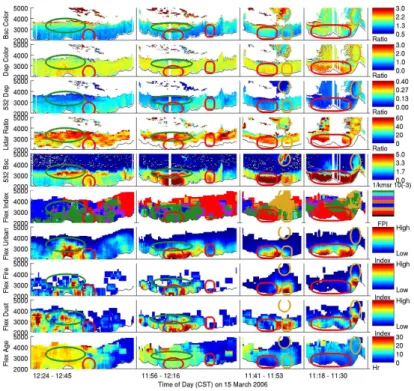
On 15 March (Fig. 9), the HSRL measured four transects starting over the southern rim of the basin and moving north. The dominant wind transport at that time is from north to south, so the transects will be displayed in reverse order to show the transport of regional pollution moving from north to south and mixing with local emissions.
The first transect detects a residual layer aloft that contains a mix of urban, biomass 5
burning and dust (green ellipse). This is an aging layer more than one day old. The red circle to the east highlights the plume of local emissions from Pachuca, a small city north of the MCMA. It extends 1000 m above ground but remains separated from the residual layer aloft.
Similar plumes can be seen in the second transect where the residual layer (second 10
green ellipse from the left margin) is now directly above local emissions at the surface from the Tula industrial region (second red ellipse from the left margin). The Pachuca plume can be seen in the red circle to the east (third from the left margin). The urban aerosols in the red circles have properties that are more similar to the ambient mix than to the urban plumes described above for 13 March.
15
The residual layer between 3000 and 4000 mm.s.l.has lower aerosol depolarization ratios at 532 nm (0.05 to 0.1, compared with 0.1 to 0.15 at the surface) and higher backscatter color ratios (1.5 to 2.5 compared with 1 to 1.5 at the surface). This sug-gests that the residual layer consists of smaller more spherical aerosols, most likely from a biomass burning plume with reduced dust content. The layer also has lower de-20
polarization color ratios (1.2 to 1.8 compared with 1.6 to 2.2 at the surface). Between 4000 and 5000 mm.s.l., an elevated plume of biomass burning smoke is beginning to be detected which will be seen more clearly in the third and fourth transects.
During the third transect, we now clearly see the urban emissions of the MCMA on the western side of the basin shown in the red ellipse (second from the right margin). 25
ACPD
10, 28471–28518, 2010Aerosol transport and transformation
with HSRL and WRF-Flexpart
B. de Foy et al.
Title Page
Abstract Introduction
Conclusions References
Tables Figures
◭ ◮
◭ ◮
Back Close
Full Screen / Esc
Printer-friendly Version Interactive Discussion
Discussion
P
a
per
|
Dis
cussion
P
a
per
|
Discussion
P
a
per
|
Discussio
n
P
a
per
|
dust (yellow ellipse from 2000 to 3000 mm.s.l.), and a purer elevated plume (yellow ellipse from 4000 to 5000 mm.s.l.). The optical properties provide a clear contrast of the two plumes, with the dust smoke mix having higher depolarization color ratios and lower backscatter color ratios whereas the purer smoke aloft has low depolarization color ratios and high backscatter color ratios.
5
The fourth transect passes south of the area influenced by biomass burning and measures urban emissions across the width of the basin (rightmost red rectangle). These are emissions from the north about to be transported over the southern basin rim and through the mountain gap in the southeast. The rightmost yellow ellipse shows the biomass burning plume on the sides of the mountains. This is lofted to 5000 mm.s.l.
10
and is the source of the high altitude plume seen in the third transect (yellow ellipse from 4000 to 5000 mm.s.l.), and also seen to a lesser degree in the first two transects.
4.4 Urban plume transport
Figures 7c and d show the maps of the HSRL transects along the plume on 3 and 13 March with the corresponding curtain plots in Figs. 10 and 11. The flight towards the 15
south on 3 March follows the plume as it is being transported over the basin rim and above the valley which is at much lower elevation (Figs. 7c and 10). Just before the top of the basin rim there is a plume extending 2000 m upwards that has the properties of dust (blue circle). The green ellipse shows the initial plume containing a mix of urban emissions, biomass burning smoke and dust. As for the transects described in 20
Sect. 4.3, the optical properties are similar to those of the mixed regional aerosols. The plume is transported in layers that remain at constant elevation, with plumes from local emissions clearly separated below.
The model simulates some fresh biomass burning plume in the vicinity of 4000 mm.s.l., shown by the two yellow ellipses. These plumes have very fine fea-25
ACPD
10, 28471–28518, 2010Aerosol transport and transformation
with HSRL and WRF-Flexpart
B. de Foy et al.
Title Page
Abstract Introduction
Conclusions References
Tables Figures
◭ ◮
◭ ◮
Back Close
Full Screen / Esc
Printer-friendly Version Interactive Discussion
Discussion
P
a
per
|
Dis
cussion
P
a
per
|
Discussion
P
a
per
|
Discussio
n
P
a
per
|
The blue circle on the right highlights a large dust plume. As with other dust plumes, the model simulates dust emissions in the area, but does not capture the very localized structure of the plume.
On 13 March (Figs. 7d and 11), the flight starts south of the basin, moves north-eastward over the gap in the basin rim and skirts the inside edge of the basin. As can 5
be seen in Fig. 7d, it does not extend as far south as the flight on 3 March. South of the basin, an elevated layer at a constant height of 3000 m can be clearly seen with the properties of the regional mix seen in the other transects (see the green circle to the left). The transport can be clearly seen in the simulations, along with the tendency of the model to move the plume along contours of constant height above ground level 10
rather than constant height above sea level.
Within the basin, the HSRL samples the urban plume as it moves south towards the gap (green rectangle). This contains a mix of urban emissions, biomass burning and dust, and has higher aerosol depolarization ratios at 532 nm than the elevated layer to the south.
15
The HSRL measures a very clear biomass burning plume above 3000 mm.s.l. (yel-low ellipse). This is correctly represented in the simulations, which shows that the plume is at most a couple of hours old. This is an example of a plume with a high de-polarization color ratio and medium-high backscatter color ratio similar to the 7 March cases (see Fig. 4), which suggests that it is mixed with dust.
20
5 Discussion
5.1 Aerosol optical properties
Table 1 presents a summary of aerosol properties measured during the MILAGRO field campaign for the main aerosol types based on the combination of data analysis and simulation comparisons. The information about aerosol morphology corresponding to 25
ACPD
10, 28471–28518, 2010Aerosol transport and transformation
with HSRL and WRF-Flexpart
B. de Foy et al.
Title Page
Abstract Introduction
Conclusions References
Tables Figures
◭ ◮
◭ ◮
Back Close
Full Screen / Esc
Printer-friendly Version Interactive Discussion
Discussion
P
a
per
|
Dis
cussion
P
a
per
|
Discussion
P
a
per
|
Discussio
n
P
a
per
|
Urban aerosols during MILAGRO had lower aerosol depolarization ratios and higher lidar ratios corresponding to more spherical and more absorbing aerosols. In contrast, dust had high aerosol depolarization ratios, low backscatter color ratios and low lidar ratios corresponding to highly non-spherical particles that are larger and absorb less. The more striking features of the analysis are the very low aerosol depolarization ratios 5
of fresh biomass burning smoke. These are combined with higher backscatter color ratios and lidar ratios suggesting small, spherical, absorbing particles. The smoke plumes during the campaign can be separated into one group consisting of pure smoke and another group consisting of mixed smoke and dust. Many of the fires around the basin were observed to be small agricultural fires in areas with bare earth and even 10
ploughing leading to dust emissions. As the biomass burning plumes aged, they were mixed with other plumes and ended up with the properties of dust.
Figure 12 shows a scatter plot of aerosol optical properties versus average particle age calculated from the simulations for the section through the gap flow on 13 March (see Figs. 11 and 7d). The HSRL measured a clear plume of mixed aerosols trans-15
ported aloft out of the basin, and a separate plume of fresh biomass burning smoke. The scattergram clearly shows the low depolarization ratios at 532 nm and high depo-larization color ratios and backscatter color ratios of the biomass burning smoke mixed with some dust. The plume was sampled very near the source, but within 10 h the optical properties have evolved to those of the mixed layer.
20
The ubiquitous presence of dust led to rapid convergence of aerosol optical proper-ties as different plumes were transported away from the source regions. In addition, complex transport patterns meant that the match between observations and simula-tions was good qualitatively, but that significant discrepancies remained in the identifi-cation and loidentifi-cation of plume features. For these two reasons, the present analysis of 25
ACPD
10, 28471–28518, 2010Aerosol transport and transformation
with HSRL and WRF-Flexpart
B. de Foy et al.
Title Page
Abstract Introduction
Conclusions References
Tables Figures
◭ ◮
◭ ◮
Back Close
Full Screen / Esc
Printer-friendly Version Interactive Discussion
Discussion
P
a
per
|
Dis
cussion
P
a
per
|
Discussion
P
a
per
|
Discussio
n
P
a
per
|
The optical properties of the aerosols sampled in and around the MCMA during MILAGRO are consistent with Querol et al. (2008) and Crounse et al. (2009) who report that there are considerable amounts of dust everywhere. Atmospheric tar balls (Posfai et al., 2004) have been detected in a number of field campaigns including MILAGRO (Yokelson et al., 2009). The very low depolarization ratios in the fresh biomass burning 5
plumes suggests that optical properties in the early plumes are dominated by very small spherical particles. This would be consistent with the presence of tar balls. As the plumes age, they are both oxidized and mixed with other aerosols, mainly dust, which would explain the rapid evolution of the properties towards larger, more irregular aerosols that are more absorbing.
10
5.2 Simulations
The results show that there is good qualitative agreement between the simulations and measurements. Nevertheless, significant discrepancies remain in the detail of the emissions and the transport. Parker (2009) suggests the use of “Adequacy-for-Purpose” when evaluating atmospheric models rather than focusing on quality of fit 15
between simulations and measurements (see also Oreskes (1998)). In the present context, we suggest that the simulations presented satisfy criteria of “Aristotelian Ac-curacy” (de Foy et al., 2009b) for identifying aerosol plumes and ages, but that direct pixel by pixel comparison is premature.
The limitations are due to uncertainties in meteorological simulations, the impact of 20
sub-grid scale effects and uncertainties in emissions models. The result is that whereas WRF-Flexpart can be used to identify large features quantitatively, and finer scale ones qualitatively, a direct mapping of HSRL measurements with Flexpart simulations con-tains too much noise to be able to detect fine changes in aerosol properties.
In terms of plume rise, even small fires were seen to have plumes extending vertically 25
ACPD
10, 28471–28518, 2010Aerosol transport and transformation
with HSRL and WRF-Flexpart
B. de Foy et al.
Title Page
Abstract Introduction
Conclusions References
Tables Figures
◭ ◮
◭ ◮
Back Close
Full Screen / Esc
Printer-friendly Version Interactive Discussion
Discussion
P
a
per
|
Dis
cussion
P
a
per
|
Discussion
P
a
per
|
Discussio
n
P
a
per
|
Localized dust storms were clearly identified in the HSRL data by the high depolar-ization ratio, low lidar ratio and low depolardepolar-ization color ratios. The small scale of these features suggests that they are generated by sub-grid scale wind fields that are not represented in the model. If a significant proportion of dust is emitted by these dust storms, this suggests that an emissions model would need to include a parametrization 5
based on sub-grid scale gust winds.
6 Conclusions
In summary, we find that the HSRL detects numerous meteorological flow features and can often provide qualitative information about aerosol types from the measurements of their optical properties. These can be used to evaluate numerical simulations of pol-10
lution transport to identify model strengths and weaknesses. The simulations capture the main flow directions of the aerosol plumes including complex venting patterns as they move inside the basin and are then vented outside of it. Vertical stratification is also represented, although we find that the model is too likely to follow the terrain rather than transport pollution plumes at constant altitude. In the measurements, there is very 15
strong layering of the plumes which the model cannot represent. This may be due to a combination of sub-grid scale effects and approximations in the planetary boundary layer schemes. With the current state of simulation accuracy, the model results can be used to identify plumes and plume aging qualitatively. Direct mapping of HSRL measurements to simulated results however still remains very approximate because of 20
mismatches in plume location.
The simulations can be used to classify the aerosol by origin and to estimate the age of the plumes. In this way, the fresh biomass burning plumes stand out as having particularly low aerosol depolarization combined with high depolarization color ratios and high backscatter color ratio. Within 10 h or less, the properties evolve to those 25
ACPD
10, 28471–28518, 2010Aerosol transport and transformation
with HSRL and WRF-Flexpart
B. de Foy et al.
Title Page
Abstract Introduction
Conclusions References
Tables Figures
◭ ◮
◭ ◮
Back Close
Full Screen / Esc
Printer-friendly Version Interactive Discussion
Discussion
P
a
per
|
Dis
cussion
P
a
per
|
Discussion
P
a
per
|
Discussio
n
P
a
per
|
for the presence of atmospheric tar balls. Dust particles start off with the opposite properties of fresh smoke: high aerosol depolarization, low backscatter color ratio and low depolarization color ratio. Given the complex combination of aerosol sources and meteorological transport, aerosols rapidly develop into mixed particulate matter with average optical properties throughout the region.
5
This work focuses on the use of particle trajectories to identify transport rather than on quantitative comparisons of concentrations. These quantitative studies are pre-cluded because we have limited the study to passive tracers with neither formation nor deposition. Nonetheless, we find that the biomass burning emission inventory from the MODIS remote sensing products detects most of the plumes measured by the HSRL. 10
We can also clearly see the rapid mixing of the urban plume within the boundary layer at the source. This transports the aerosol aloft which then get stratified as the free tropospheric flow exports the plumes regionally. The plume rise from biomass burning was also evident leading to transport aloft. Dust storms were equally found to have con-siderable vertical extent, although in contrast with the biomass burning plumes, these 15
do not persist at higher elevations suggesting that there is rapid deposition. Overall, the combination of measurements and numerical simulations provides detailed information on aerosol properties that can be used to explore plume transport and transformation as well as numerical model behavior.
Supplementary material related to this article is available online at:
20
http://www.atmos-chem-phys-discuss.net/10/28471/2010/ acpd-10-28471-2010-supplement.pdf.
Acknowledgements. We wish to thank the large number of people involved in the MILAGRO field campaign as well as those involved in monitoring in the Mexico City basin without which this study would not exist.
25
ACPD
10, 28471–28518, 2010Aerosol transport and transformation
with HSRL and WRF-Flexpart
B. de Foy et al.
Title Page
Abstract Introduction
Conclusions References
Tables Figures
◭ ◮
◭ ◮
Back Close
Full Screen / Esc
Printer-friendly Version Interactive Discussion
Discussion
P
a
per
|
Dis
cussion
P
a
per
|
Discussion
P
a
per
|
Discussio
n
P
a
per
|
and the Molina Center for Strategic Studies in Energy and the Environment is gratefully ac-knowledged for this work.
We acknowledge the support of the NASA LaRC, NASA HQ Science Mission Directorate, and the NASA CALIPSO Project for funding the development of the HSRL instrument. The deploy-ment of the HSRL in these field experideploy-ments were supported in part by the US Departdeploy-ment of
5
Energys Atmospheric Science Program (Office of Science, BER, Grant DE-AI02-05ER63985). We also acknowledge the aircraft flight support provided by personnel in the NASA LaRC Re-search Services Directorate.
References
Adachi, K. and Buseck, P. R.: Internally mixed soot, sulfates, and organic matter in aerosol
10
particles from Mexico City, Atmos. Chem. Phys., 8, 6469–6481, doi:10.5194/acp-8-6469-2008, 2008. 28474
Aiken, A. C., Salcedo, D., Cubison, M. J., Huffman, J. A., DeCarlo, P. F., Ulbrich, I. M., Docherty, K. S., Sueper, D., Kimmel, J. R., Worsnop, D. R., Trimborn, A., Northway, M., Stone, E. A., Schauer, J. J., Volkamer, R. M., Fortner, E., de Foy, B., Wang, J., Laskin, A., Shutthanandan,
15
V., Zheng, J., Zhang, R., Gaffney, J., Marley, N. A., Paredes-Miranda, G., Arnott, W. P., Molina, L. T., Sosa, G., and Jimenez, J. L.: Mexico City aerosol analysis during MILAGRO using high resolution aerosol mass spectrometry at the urban supersite (T0) – Part 1: Fine particle composition and organic source apportionment, Atmos. Chem. Phys., 9, 6633–6653, doi:10.5194/acp-9-6633-2009, 2009. 28474
20
Aiken, A. C., de Foy, B., Wiedinmyer, C., DeCarlo, P. F., Ulbrich, I. M., Wehrli, M. N., Szidat, S., Prevot, A. S. H., Noda, J., Wacker, L., Volkamer, R., Fortner, E., Wang, J., Laskin, A., Shutthanandan, V., Zheng, J., Zhang, R., Paredes-Miranda, G., Arnott, W. P., Molina, L. T., Sosa, G., Querol, X., and Jimenez, J. L.: Mexico city aerosol analysis during MILAGRO using high resolution aerosol mass spectrometry at the urban supersite (T0) – Part 2: Analysis of
25
the biomass burning contribution and the non-fossil carbon fraction, Atmos. Chem. Phys., 10, 5315–5341, doi:10.5194/acp-10-5315-2010, 2010. 28475, 28482
ACPD
10, 28471–28518, 2010Aerosol transport and transformation
with HSRL and WRF-Flexpart
B. de Foy et al.
Title Page
Abstract Introduction
Conclusions References
Tables Figures
◭ ◮
◭ ◮
Back Close
Full Screen / Esc
Printer-friendly Version Interactive Discussion
Discussion
P
a
per
|
Dis
cussion
P
a
per
|
Discussion
P
a
per
|
Discussio
n
P
a
per
|
in atmospheric models, Atmos. Chem. Phys. Discuss., 10, 27523–27602, doi:10.5194/acpd-10-27523-2010, 2010. 28482
Al-Saadi, J., Soja, A., Pierce, R. B., Szykman, J., Wiedinmyer, C., Emmons, L., Kondragunta, S., Zhang, X., Kittaka, C., Schaack, T., and Bowman, K.: Intercomparison of near-real-time biomass burning emissions estimates constrained by satellite fire data, J. Appl. Remote
5
Sens., 2, 021504, doi:10.1117/1.2948785, 2008. 28482
Alexander, D. T. L., Crozier, P. A., and Anderson, J. R.: Brown carbon spheres in East Asian outflow and their optical properties, Science, 321, 833–836, doi:10.1126/science.1155296, 2008. 28476
Andreae, M. and Merlet, P.: Emission of trace gases and aerosols from biomass burning, Global
10
Biogeochem. Cy., 15, 955–966, 2001. 28482
Burton, S. P., Ferrare, R. A., Hostetler, C. A., Hair, J. W., Kittaka, C., Vaughan, M. A., Obland, M. D., Rogers, R. R., Cook, A. L., Harper, D. B., and Remer, L. A.: Using airborne high spec-tral resolution lidar data to evaluate combined active plus passive retrievals of aerosol ex-tinction profiles, J. Geophys. Res.-Atmos., 115, D00H15, doi:10.1029/2009JD012130, 2010.
15
28478
Cattrall, C., Reagan, J., Thome, K., and Dubovik, O.: Variability of aerosol and spectral lidar and backscatter and extinction ratios of key aerosol types derived from selected Aerosol Robotic Network locations, J. Geophys. Res.-Atmos., 110, D10S11, doi:10.1029/2004JD005124, 2005. 28480
20
Chakrabarty, R., Moosmuller, H., Garro, M., Arnott, W., Walker, J., Susott, R., Babbitt, R., Wold, C., Lincoln, E., and Hao, W.: Emissions from the laboratory combustion of wildland fuels: Particle morphology and size, J. Geophys. Res.-Atmos., 111, D07204, doi:10.1029/ 2005JD006659, 2006. 28476
Chakrabarty, R. K., Moosm ¨uller, H., Chen, L.-W. A., Lewis, K., Arnott, W. P., Mazzoleni, C.,
25
Dubey, M. K., Wold, C. E., Hao, W. M., and Kreidenweis, S. M.: Brown carbon in tar balls from smoldering biomass combustion, Atmos. Chem. Phys., 10, 6363–6370, doi:10.5194/acp-10-6363-2010, 2010. 28476
Christian, T. J., Yokelson, R. J., C ´ardenas, B., Molina, L. T., Engling, G., and Hsu, S.-C.: Trace gas and particle emissions from domestic and industrial biofuel use and garbage burning
30
in central Mexico, Atmos. Chem. Phys., 10, 565–584, doi:10.5194/acp-10-565-2010, 2010. 28475
ACPD
10, 28471–28518, 2010Aerosol transport and transformation
with HSRL and WRF-Flexpart
B. de Foy et al.
Title Page
Abstract Introduction
Conclusions References
Tables Figures
◭ ◮
◭ ◮
Back Close
Full Screen / Esc
Printer-friendly Version Interactive Discussion
Discussion
P
a
per
|
Dis
cussion
P
a
per
|
Discussion
P
a
per
|
Discussio
n
P
a
per
|
de M ´exico, Tech. Rep. (Web), Secretar´ıa del Medio Ambiente, Gobierno de M ´exico, M ´exico, 2008. 28481
Crounse, J. D., DeCarlo, P. F., Blake, D. R., Emmons, L. K., Campos, T. L., Apel, E. C., Clarke, A. D., Weinheimer, A. J., McCabe, D. C., Yokelson, R. J., Jimenez, J. L., and Wennberg, P. O.: Biomass burning and urban air pollution over the Central Mexican Plateau, Atmos.
5
Chem. Phys., 9, 4929–4944, doi:10.5194/acp-9-4929-2009, 2009. 28475, 28493
de Foy, B., Caetano, E., Maga ˜na, V., Zit ´acuaro, A., C ´ardenas, B., Retama, A., Ramos, R., Molina, L. T., and Molina, M. J.: Mexico City basin wind circulation during the MCMA-2003 field campaign, Atmos. Chem. Phys., 5, 2267–2288, doi:10.5194/acp-5-2267-2005, 2005. 28477
10
de Foy, B., Clappier, A., Molina, L. T., and Molina, M. J.: Distinct wind convergence patterns in the Mexico City basin due to the interaction of the gap winds with the synoptic flow, Atmos. Chem. Phys., 6, 1249–1265, doi:10.5194/acp-6-1249-2006, 2006a. 28474
de Foy, B., Molina, L. T., and Molina, M. J.: Satellite-derived land surface parameters for mesoscale modelling of the Mexico City basin, Atmos. Chem. Phys., 6, 1315–1330,
15
doi:10.5194/acp-6-1315-2006, 2006b. 28481
de Foy, B., Varela, J. R., Molina, L. T., and Molina, M. J.: Rapid ventilation of the Mex-ico City basin and regional fate of the urban plume, Atmos. Chem. Phys., 6, 2321–2335, doi:10.5194/acp-6-2321-2006, 2006c. 28474
de Foy, B., Lei, W., Zavala, M., Volkamer, R., Samuelsson, J., Mellqvist, J., Galle, B., Mart´ınez,
20
A.-P., Grutter, M., Retama, A., and Molina, L. T.: Modelling constraints on the emission inven-tory and on vertical dispersion for CO and SO2in the Mexico City Metropolitan Area using So-lar FTIR and zenith sky UV spectroscopy, Atmos. Chem. Phys., 7, 781–801, doi:10.5194/acp-7-781-2007, 2007. 28483
de Foy, B., Fast, J. D., Paech, S. J., Phillips, D., Walters, J. T., Coulter, R. L., Martin, T. J., Pekour,
25
M. S., Shaw, W. J., Kastendeuch, P. P., Marley, N. A., Retama, A., and Molina, L. T.: Basin-scale wind transport during the MILAGRO field campaign and comparison to climatology using cluster analysis, Atmos. Chem. Phys., 8, 1209–1224, doi:10.5194/acp-8-1209-2008, 2008. 28473, 28477
de Foy, B., Krotkov, N. A., Bei, N., Herndon, S. C., Huey, L. G., Mart´ınez, A.-P., Ruiz-Su ´arez,
30