www.atmos-chem-phys.net/8/159/2008/ © Author(s) 2008. This work is licensed under a Creative Commons License.
Chemistry
and Physics
Scanning rotational Raman lidar at 355 nm for the measurement of
tropospheric temperature fields
M. Radlach, A. Behrendt, and V. Wulfmeyer
University of Hohenheim, Institute of Physics and Meteorology, Garbenstrasse 30, 70599 Stuttgart, Germany Received: 14 March 2007 – Published in Atmos. Chem. Phys. Discuss.: 31 May 2007
Revised: 16 November 2007 – Accepted: 12 December 2007 – Published: 15 January 2008
Abstract. For high-resolution measurements of tempera-ture fields in the atmospheric boundary layer and the lower free troposphere a scanning eye-safe lidar which deploys the rotational Raman technique at 355 nm was developed. To optimize the filters of the receiver for both high nighttime and daytime performance, detailed simulation studies have been performed. The receiver is fiber-coupled to a sequential setup of multicavity interference filters used under small an-gles of incidence. Examples of nighttime and daytime mea-surements with the system which has a total power-aperture-efficiency product of 0.006 W m2 are presented. Noontime temperature measurements with a temporal resolution of 60 s result in 1-sigma statistical temperature uncertainty of<1 K up to 1 km height and <2 K up to 2 km height. With an integration time of 60 min and a gliding average of 750 m a 1-sigma statistical temperature uncertainty of<1 K up to 14 km height is achieved during night.
1 Introduction
Temperature is a key parameter to describe the state of the atmosphere. It rules atmospheric stability. The observation of the diurnal variation of temperature layering in the free troposphere and the boundary layer is important for many meteorological processes e.g. the initiation of convection or the propagation of gravity waves. Thus for a comprehen-sive understanding of such processes, we developed an in-strument which is capable of measuring temperature from close to the ground up to the tropopause with high accuracy and high temporal and spatial resolution. A scanner allows to perform these measurements in any direction of interest and hence to investigate spatial variability, especially, inside the Correspondence to:M. Radlach
atmospheric boundary layer and of the transition to the free troposphere.
The rotational Raman (RR) lidar technique for the mea-surement of atmospheric temperature was suggested by Cooney (1972). It makes use of the temperature dependence of the intensities of the rotational Raman lines. At date, the RR technique is the most reliable lidar method for temper-ature profiling (Behrendt, 2005) in the troposphere. Sev-eral ground based systems exist today (Vaughan et al., 1993; Nedeljkovic et al., 1993; Behrendt and Reichardt, 2000; Mat-tis at al., 2002) and even airborne (Behrendt et al., 2004a) and space-borne (Di Girolamo et al., 2006) application seems feasible.
Besides the RR technique also high spectral resolution li-dar (HSRL) is used to measure tropospheric temperature pro-files. The HSRL technique is resolving the temperature de-pendent linewidth of the Cabannes line which is Doppler broadened (Schwiesow and Lading, 1981; Shimizu et al., 1983). This technique poses much higher demands in re-spect to the stability of the system as shown in Hair et al. (2001) than RR lidar. Furthermore, it is difficult to achieve sufficiently high rejection of the Mie scattering (Hua et al., 2005a,b). While with the rotational Raman technique and state of the art interference filters, even measurements in optically thin clouds are possible (Behrendt and Reichardt, 2000).
So far, RR lidar systems have mainly been operated at the frequency-doubled wavelength of Nd:YAG lasers of 532 nm because of the higher laser power and receiver efficiency at this wavelength compared to the UV. Such systems are at date capable of temperature profiling up to the upper strato-sphere (Behrendt et al., 2004b). In principle, UV wave-lengths are advantageous to visible wavewave-lengths because the rotational Raman backscatter coefficient is proportional to λ−4. Attempts have also been made to use an UV wavelength
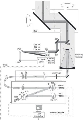
Fig. 1.Schematic setup of the scanning rotational Raman lidar sys-tem of UHOH. BD: beam dump, BE: beam expander, BSU: Scanner (beam steering unit), IF0–IF3: interference filter, L1–L6: lenses, LM: laser mirrors, ND: neutral density filter, OF: optical fiber, PBP: Pellin-Broca prism, PMT: photomultiplier tube, TRIG: trigger sig-nal.
knowledge were made by Di Girolamo et al. (2004) with the frequency-tripled radiation of Nd:YAG laser of 355 nm. Day-time temperature profiling was demonstrated in the visible with gratings combined with a Fabry-Perot interferometer as a comb-filter (Arshinov et al., 2005) and with narrow-band interference filters (Behrendt et al., 2002; Di Girolamo et al., 2004). The better optical performance for narrow-band in-terference filters in the UV that can be realized today leads to a better system performance for tropospheric tempera-ture profiling than for comparable systems in the visible do-main because of the higher molecular backscatter coefficient and a higher efficiency of the detectors at lower wavelengths (Behrendt, 2005).
At University of Hohenheim (UHOH) we have developed a highly efficient RR lidar in the UV with a cascade filter mounting which is optimized for temperature measurements in the lower troposphere. This RR receiver setup was first
introduced by Behrendt and Reichardt (2000) and was oper-ated before only at 532 nm. In Sect. 2 the system setup of our scanning RR lidar is described. Section 3 gives a short overlook of the simulation of the filter parameters which we performed in order to select filter parameters optimized for our purposes. An example of a nighttime and a daytime as well as a scanning measurement is presented in Sects. 4–6. Conclusions are given in Sect. 7.
2 System setup
Table 1.Technical data.
Laser
Type Flash-lamp-pumped frequency tripled Nd:YAG laser, Spectra-Physics GCR5-30
Wavelength 354.66 nm
Pulse energy ≈300 mJ
Pulse repetition rate 30 Hz
Pulse duration 10 ns
Receiver
Geometry Ritchey-Chretien telescope
Primary mirror diameter 0.4 m Telescope focal length 4 m
Field of view 0.75 mrad (selectable) Polychromator
Detectors Hamamatsu R7400-U02 (elastic channel) Hamamatsu R1924P (rotational Raman channels) Data acquisition system 3 channel Licel Transient recorder
TR40-40 (analog and photon-counting) + opt-PR 2.5–20
we use two filters for the first rotational Raman channel. As shown in Table 2, already one order of suppression of the elastically scattered light is obtained at IF1 which reflects less than 10 % at the laser wavelength. The temperature is calculated with the ratioQ(T )=PRR1(R, T )/PRR2(R, T )of
the two RR signalsPRR1(T , R)andPRR2(T , R)which
de-pend on rangeRand temperatureT.
An estimation results in a power-aperture-efficiency product of about 0.006 W m2for the full system including all optical components but the narrow-band interference filters IF1–IF3 which have peak transmissions of 0.62, 0.34 and 0.52 for the elastic, RR1 and RR2 channel, respectively. The values are mostly taken from manufacturers’ data sheets but the reflec-tivities for the 3 consecutive laser mirros (LM) and both of the large scanner mirrors (Fig. 1) were measured by the au-thors.
The rotational Raman signals are extracted from the anti-Stokes branch like done before with other systems (Nedeljkovic et al., 1993; Behrendt and Reichardt, 2000; Behrendt et al., 2002; Di Girolamo et al., 2004). The trans-mission curves of the filters manufactured by Barr Asso-ciates, MA, USA, and the pure rotational Raman spectrum for N2and O2at temperatures of 250 K and 300 K are shown
in Fig. 2. The filter parameters are listed in Table 2. They were selected according to the results of detailed optimiza-tions described in Sect. 3.
The data acquisition is performed with a 3-channel transient recorder of Licel GmbH, Germany. The data of each chan-nel are recorded as three signals: with 3.75 m resolution up to range of 15 km in analog and photon-counting mode and simultaneously in photon-counting mode with 37.5 m reso-lution up to a range of 76.8 km. This concept allows us to use the analog signals in the near range in which the
photon-353 354 355 356 357
0.5 1.0
25 50 75 100
0
N2 O2
300 K 250 K
.
u .
a ,
yti
s
n
et
nI
Wavelength, nm
IF1 IF2a IF2b IF2a+2b IF3
% ,
n
oi
ss
i
ms
na
r
T
λ
Fig. 2. Transmission curves of the narrow-band interference fil-ters used in the rotational Raman lidar polychromator together with the rotational Raman spectrum of N2and O2for temperatures of
T1=300 K andT2=250 K.λ0denotes the wavelength of the laser.
counting signals are saturated and the photon-counting sig-nals in far range in which the signal-to-noise ratio of the ana-log data is low. It is then possible to combine the anaana-log and the photon-counting data to get a single profile (e.g. Behrendt et al., 2004b; Whiteman et al., 2006; Pety et al., 2006).
3 Filter optimization
352.4 352.6 352.8 353.0 353.2 353.4 353.6 353.8 λCWL2, nm
353.8 354.0 354.2 354.4 354.6 λ 1 L W C , m n 1.00 1.05 1.10 1.15 1.20 1.25 1.30 1.35 1.40 1.45 1.50 > T=300 K
a
352.4 352.6 352.8 353.0 353.2 353.4 353.6 353.8 λCWL2, nm
353.8 354.0 354.2 354.4 354.6 λ 1 L W C , m n 1.0 1.1 1.2 1.3 1.4 1.5 1.6 1.7 1.8 1.9 2.0 > T=300 K
d
352.4 352.6 352.8 353.0 353.2 353.4 353.6 353.8 λCWL2, nm
353.8 354.0 354.2 354.4 354.6 λ 1 L W C , m n 1.00 1.05 1.10 1.15 1.20 1.25 1.30 1.35 1.40 1.45 1.50 > T=270 K
b
352.4 352.6 352.8 353.0 353.2 353.4 353.6 353.8
λCWL2, nm
353.8 354.0 354.2 354.4 354.6 λ 1 L W C , m n 1.0 1.1 1.2 1.3 1.4 1.5 1.6 1.7 1.8 1.9 2.0 > T=270 K
e
1.00 1.05 1.10 1.15 1.20 1.25 1.30 1.35 1.40 1.45 1.50 >352.4 352.6 352.8 353.0 353.2 353.4 353.6 353.8 λCWL2, nm
353.8 354.0 354.2 354.4 354.6 λ 1 L W C , m n T=220 K
c
1.0 1.1 1.2 1.3 1.4 1.5 1.6 1.7 1.8 1.9 2.0 >352.4 352.6 352.8 353.0 353.2 353.4 353.6 353.8 λCWL2, nm
353.8 354.0 354.2 354.4 354.6 λ 1 L W C , m n T=220 K
f
Fig. 3.Results of the optimization calculations for the parameters of the rotational Raman channel filters: Calculated statistical temperature uncertainty1T versus filter CWLsλCWL1andλCWL2for the filters shown in Fig. 2. Left:(a)(T1, T2)=(300 K, 305 K),(b)(T1, T2)=(270 K,
275 K) and(c)(T1, T2)=(220 K, 225 K). Right: same as (a–c) but with a background signal of the same intensity as the strongest rotational
Raman line in the anti-Stokes branch added to the signals. Calculation step width was 0.01 nm. Values for1T are scaled relatively to the minimum () of each plot. The circle marks our setup. The gray scale of1T is plotted on the right.
maximum) at different atmospheric temperaturesT. For the calculations we took into account the RR lines of N2and O2.
The 1-σ statistical temperature uncertainty can be calculated with
1T = ∂T
∂Q1Q (1)
≈ (T1−T2)
(Q1−Q2)
Q s
PRR1+2PB1
PRR12
+PRR2+2PB2
PRR22
,
withPRR1andPRR2for the background corrected RR signals
andQthe ratio of these two signals (Behrendt et al., 2004b). We calculated the uncertainties for different pairs of temper-ature (T1, T2) ranging from (220, 225 K) to (300, 305 K).
Q1andQ2are the corresponding ratio values of the two
ex-tracted RR signals. PB1 andPB2 are the total background
signals of each RR signal due to both detector noise and
so-lar background. The statistical temperature uncertainties are minimum for a certain combination of high temperature sen-sitivity and large signal intensities dependent on temperature and background intensity.
We fulfilled different steps to attain our current filter spec-ification. In the first step, we used a modified Gaussian curve to extract the signals out of the anti-Stokes branch in the sim-ulations. The function is defined by
f (λ)=Aexp "
−
2(λ−λCWL) B
1λFWHM
4#
(2)
withλCWLthe central wavelength at the peak transmissionA
and1λFWHM the filter width. B is describing the shape of
Table 2.Filter parameters.
IF0 IF1 IF2a IF2b IF3
AOI, deg 0.0 5.7 6.5 6.5 6.2
CWL, nm 353.65 354.66 354.05 354.05 353.05
FWHM, nm 8.5 0.29 0.32 0.33 0.52
Peak transmission 0.56 0.62 0.53 0.65 0.52
Reflectivity at 354.66 nm <0.1
Transmission at 354.66 nm 0.56 0.62 <10−3 <10−3 <10−6
curve include very steep edges and an idealized transmission of 100% (A=1). To simulate daytime performance, we used a background signal per 0.1 nm of the spectrum which we scaled with a factorSrelative to the intensity of the strongest RR line in the anti-Stokes branch. The background of each channel was then calculated for the respective filter width 1λFWHM. We get therefore
PB=S
λFWHM
0.1nmP
max
J (3)
withPJmaxas intensity of the strongest RR line in the anti-Stokes branch and1λFWHMthe filter width.
First calculations showed us that the most inappropri-ate filter bandwidth is at around 0.1 nm. For such nar-row filters there is never more than one RR line of N2
within the extracted signal because the RR lines are sep-arated by >0.1 nm for a primary wavelength of 355 nm. The simulations showed that a pair of broader filters with different FWHM is the best choice. Below, 1λFWHM1
is corresponding to the filter that extracts the RR signals close to the laser wavelength in the channel RR1 (in our case the pair of filters IF2a and IF2b) and 1λFWHM2
cor-responds to the filter which extracts the RR signals of higher rotational quantum states in the channel RR2 (IF3 in our case). When comparing equal transmission values
1λFWHM1=1λFWHM2=0.05 nm with broader filters with
1λFWHM1=0.3 nm and 1λFWHM2=0.5 nm we found much
lower statistical uncertainties in case of no background for the broader filters. This is due to the higher number of se-lected RR lines. But even with daylight background, 1T for the broader pair of filters is almost equal to the pair with
1λFWHM1=1λFWHM2=0.05 nm regardless of the intensity
of the background. It is worth mentioning that transmis-sion values for very narrow filters with FWHM=0.05 nm are feasible with around 15–20% at date. While filters with FWHM>0.3 nm can be manufactured with a transmission higher than 60%.
In the second step, we used realistic filter curves for our favored filter bandwidths of 0.3 nm for the first RR channel and 0.5 nm for the second RR channel. The filter curves were provided by Barr Associates, MA, USA, and included a real-istic shape and transmission. In an iterative process, we opti-mized the CWL for low statistical measurement errors of RR
0
2
4
6
8
10
12
10
-310
-210
-110
010
110
210
3P
BG, Lidar
/P
BHeight, km a.g.l.
RR1
RR2
S=0.1
S=1
S=10
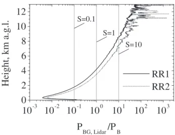
Fig. 4. Comparison of a measured daylight background in the RR channels RR1 and RR2 measured on 11 July 2006 at Hornisgrinde, 1161 m above sea level (a.s.l.) (Black Forest, Germany) between 11:30– 12:15 UTC to the simulated background PB. Local noon
is at 11:33 UTC. The ratio PBG,Lidar/PB is equal to the value of
S which needs to be selected to obtain the measured background according to Eq. (3) for the simulation.
temperature measurement under the condition to get at the same time sufficient suppression of at least 7 orders of mag-nitude of the elastically backscattered light in the RR chan-nels. The optimum CWL we found for this configuration of filter pairs were ordered for an angle of incidence (AOI) of 5◦to allow the sequential mounting and wavelength tuning.
In the last step finally the optimum setup was simu-lated with the transmission curves of the manufactured fil-ters (see Fig. 2 and Table 2) by calculating 1T with Eq. (1). The calculations for atmospheric temperatures of (T1, T2)=(300 K, 305 K), (T1, T2)=(270 K, 275 K) and
(T1, T2)=(250 K, 255 K) are shown without and with
back-ground signal in Fig. 3a–c and Fig. 3d–f, respectively. These simulations were performed for the wavelength of our laser of 354.66 nm. Figures 3a–c and Figs. 3d–f show that there is a pronounced shift of the optimumλCWL2towards longer
∆
T, K
0 1 2 3 4 5
255 270 285 -2 0 2
a
Lidar
11:52-12:12 UTC Local Radiosonde 12 UTC
Temperature, K
Height, km a.g.l.
b
Signal smoothing 0.0 - 1.5 km: 120 m 1.5 - 5.0 km: 600 m
∆TLidar T
Lidar- TRS
Fig. 5. Time-height cross section of 60-s temperature profiles be-tween 11:52–12:12 UTC on 27 March 2006 at University of Ho-henheim (Stuttgart, Germany) (left) and lidar profile with error bars (straight line) from 11:56 UTC and radiosonde (circles) from 12:00 UTC (right). Lidar signals were smoothed with a gliding average of 240 m. Error bars show the statistical temperature uncer-tainty.
only a very small shift forλCWL1for the temperature range
investigated. In case of daytime performance in Fig. 3d– f with S=1 there is a shift towards longer wavelengths of λCWL2 and a shift towards shorter wavelengths of λCWL1
compared to the case without background (Fig. 3a–c). This shift also is barely increasing in case ofS≫1. In conclusion, Fig. 3 show that we can fixλCWL1at one position and we
afterwards can improve the system sensitivity by changing λCWL2 by selecting the AOI depending on the background
level present at the temperature range of interest. This can be done without any further adjustments of the other channels because the second RR channel is the last in the sequence. For the measurements presented in this paper, however, we decided to keep the filters fixed for optimum daytime perfor-mance and have not yet made use of this method for further improvements for nighttime measurements.
We had to offsetλCWL1towards a shorter wavelength
be-cause of sufficient suppression of the elastic scattered light at the optimum position. For a temperature of 300 K this leads to an increase of statistical temperature uncertainties of just about 17% and 8% without and with daylight back-ground, respectively. We obtain high performance in the lower troposphere like it is our goal. For other temperatures we got the following results: 270 K, uncertainties increase by 15% and 11% without and with daylight background, re-spectively; 220 K, uncertainties increase by 13% and 36% without and with daylight background, respectively.
To show that the artificial background signal used for the
filter simulations is realistic, a typical measurement signal is compared with the simulations. The solar elevation angle was about 60◦during the lidar measurement.
For comparison it is necessary to scale the theoretical derived background relatively to the measured background. This is done byPLidar/PSimulation×PB. Figure 4 shows the
ratio of the measured background signalsPBG,Lidarto the
the-oreticalPB. It turns out that the simulations with the
artifi-cial background is matching the reality at about 4 km alti-tude. This height gives the point in whichPLidar/PBG,Lidaris
just equal toPSimulation/PB. Here the temperature was 267 K
in this case. AsPLidaris range-dependent andPSimulationis
not a scaling factor of S=1 used for Fig. 3d–f is too high for heights below 4 km and too low above. It is important to note, that this does not affect our conclusions since no sig-nificant changes in optimum filter parameters were found for even much higher values ofS. IfS is matched to simulate the performance for higher temperatures (e.g. for heights at around 1.5 kmS=0.1, which corresponds to a temperature of 285 K in that case) the optimum values forλCWL2is shifted
towards shorter wavelength by 0.1 nm whereasλCWL1is not
changed. In summary it can be stated that the performance simulations show that we can select filter parameters close to the optimum with and without daylight background and for a large range of temperatures.
4 Daytime measurements
The measurement example presented in this section is from 27 March 2006 at the site of University of Hohenheim, Stuttgart, Germany. The data were acquired at about noon between 11:52 and 12:12 UTC.
The lidar needs to be calibrated to obtain temperature. This is done by comparison of the ratio Q(T )of the two RR signals with temperature profiles measured with ra-diosondes that are close in time and space to the lidar mea-surement. For the calibration we useQ(T )=exp(a/T+b) which is the exact function of Q(T )for two isolated lines (Behrendt, 2005),T is temperature anda,bare calibration constants. We found in this case no differences worth con-sidering the more complicated expression (Behrendt et al., 2002)Q(T )=exp(a′/T2
+b′/T+c′).
∆
∆
265 275 285
11:55 12:00 12:05 12:10 1.0
1.5 2.0
Time, UTC
Height, km a.g.l.
270 272 274 276 278 280 282 284 286 288
11:56 UTC Lidar
Temperature, K
Local Radiosonde 12 UTC
T, K
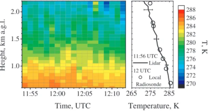
Fig. 6. (a)Lidar and radiosonde temperature profiles measured on 27 March 2006 at University of Hohenheim (Stuttgart, Germany). Lidar signals were smoothed with a gliding average of the indicated window lengths. Error bars are showing the statistical temperature uncertainty of the lidar profile. (b)Difference between lidar and radiosonde temperature and 1-σtemperature uncertainty of the lidar profile.
11:55 12:00 12:05 12:10
1.0 1.5 2.0
1.0 1.5 2.0
−1
1
0
Time, UTC
Height, km a.g.l.
d ln[P(z) z²]/dz, a.u.
Fig. 7.Time-height cross section of the logarithm of the range cor-rected elastic signal on 27 March 2006 at University of Hohenheim (Stuttgart, Germany). The black line marks the boundary layer top.
Figure 5b shows the deviations between the lidar profile and the radiosonde as well as the statistical temperature uncer-tainty of the lidar profile. In this case the deviations are al-ways smaller than 1-σuncertainties of the lidar profile except at heights below 1 km above ground layer (a.g.l.) which are caused by natural differences in the boundary layer. The 1-σ statistical temperature uncertainties are not exceeding 3 K up to 5 km altitude a.g.l. and they are less than 1 K up to 3 km a.g.l. Figure 6 shows the time-height cross section of the 20-min time series. The profile of 11:56 UTC is shown on the right side. The statistical uncertainties are not exceed-ing 1 K up to 1 km a.g.l. and are well below 3 K up to 2 km height. The time-height cross section of the gradient of the logarithm of the range-corrected elastically scattered light as well as the temperature gradient is plotted in Figs. 7 and 8, respectively. From the data shown in Fig. 7 the boundary layer top was determined (black line). It can be seen that it is varying between 1.7 and 2.0 km a.g.l. during the mea-surement period. Normally the BL top is well defined by a temperature inversion or a lid. Such a lid is existing in the
11:55 12:00 12:05 12:10
1.0 1.5 2.0
1.0 1.5 2.0
−10
−8
−6
−4
−2
Time, UTC
Height, km a
.g.l
. dT/
dz
,
K/
k
m
Fig. 8.Time-height cross section of the temperature gradient on 27 March 2006 at University of Hohenheim (Stuttgart, Germany). The black line is marking the boundary layer top derived by Fig. 7.
region of the BL top like seen in Fig. 8 with the temperature gradient. Values between −0.1 and 0.4 K/100 m mark the stable region which correlates with the BL top derived with the aerosol data.
5 Nighttime measurement: vertical
The measurement example shown in this and the following section were carried out during a campaign in the northern Black Forest in Germany. The campaign took place from 6– 21 July 2006. The lidar site was situated on Hornisgrinde, the highest peak in the Northern Black Forest (8.2◦E, 48.6◦N)
with an elevation of 1161 m above sea level (a.s.l.). During the campaign, radiosondes were launched in a distance of 3 km west of the lidar site at Brandmatt. This station was situated in a valley at an elevation of around 700 m a.s.l.
Table 3.Lidar temperature versus radiosonde at height intersections for the measurement example shown in Fig. 11.
Scan number Range to Spatial distance TRS TLidar 1TLidar TLidar−TRS radiosonde of measurement points
lidar–radiosonde
5 4.6 km 1.3 km 273.3 K 274.0 K 0.6 K 0.7 K
6 2.1 km 0.8 km 283.0 K 284.7 K 0.5 K 1.7 K
7 2.2 km 1.0 km 284.5 K 285.2 K 0.5 K 0.7 K
8 2.7 km 1.0 km 284.7 K 283.9 K 0.7 K 0.8 K
9 3.0 km 0.6 km 290.1 K 288.9 K 0.7 K 1.6 K
0 4 8 12 16 20 24
220 240 260 280 300 -6 -3 0 3 6
b
a
Radiosonde Brandmatt 21 UTC
Munich 0 UTC
Temperature, K
Height, km a.g.l.
Lidar, 20-21 UTC
TLidar-TMunich
∆TLidar
T
Lidar-TBrandmatt
∆
T, K
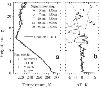
Signal smoothing150 m 0 - 3 km:
450 m 3 - 7 km:
750 m 7 - 20 km:
1500 m 12 - 20 km:
3000 m 20 - 25 km:
Fig. 9. (a)Lidar and radiosonde temperature profiles during night on 10 July 2006 on Hornisgrinde (Black Forest, Germany). Lidar signals were initially smoothed with a gliding average of the indi-cated window lengths. Error bars show the statistical temperature uncertainty of the photon-counting data. (b) Difference between lidar and the local radiosonde launched in Brandmatt and 1-σ tem-perature uncertainty.
temperature uncertainties above 14 km altitude. Larger dif-ferences of about 4 K between 16 and 19 km height might be caused by gravity wave activity above the lidar site.
The drift of the radiosonde during this ascent was mainly affected by a slow flow of 2–9 m/s. Up to 3 km a.s.l. the drift was basically towards the east. Beyond that level the sonde started circling around Hornisgrinde in a distance of 1–2 km by drifting to the southeast up to 5 km a.s.l. Above that level the ascent continued steadily northeastward. Up to a height of 9 km the sonde was within a circle of 3 km to the lidar site. It should be pointed out that the prominent feature of these deviations here is apparently wave-like (1T maxima in equidistant height of 2, 4, 6, 8 and 10 km) which coincides with the fact that the meteorological conditions were favor-able for orographically induced gravity waves on that day.
0
−1 −2
−3 1 2 3
1000 2000 3000
Height, m a.s.l.
Horizontal Distance, km
1161 m, Lidar Site→ Ε
W ←
1
2
3
4
5
6
7
8
9
4000
← ←
Track of Radiosonde
Fig. 10.Scan pattern and W-E cross section through the lidar site. Numbers from 1–9 are denoting directions in which profiles were measured. The track of the local radiosonde transposed to this plane, launched at 21:10 UTC, is illustrated by the dotted line.
6 Nighttime measurement: scanning
As first rotational Raman lidar, the system allows scanning measurements to investigate the variability of the temper-ature field. A scan pattern which we performed during a radiosonde launch is shown in Fig. 10. In the case pre-sented here from 10 July 2006 we performed a zonal-RHI-scan (Range-Height-Indicator) with a constant step width of 22.5◦. The lidar data was collected between 21:00 and
22:00 UTC. The temporal resolution for each pointing di-rection was 60 s. We performed 6 scans during the one-hour measurement period which were added up to improve the sig-nal statistics. For the calculation of temperature profiles we used the calibration constants determined by the measure-ment in Sect. 5.
0 1 2 3 4
0 1 2 3 4
0 1 2 3 4
275 280 285 290 275 280 285 290 275 280 285 290
1.5 2.0 2.5
2 3
2 3 4
2 3 4 5
2 3 4
2 3
1.5 2.0 2.5
9
8
7
6
5
4
3
2
1
Range, km
Range, km
Temperature, K
Range, km
Temperature, K
Temperature, K
Height, km a.s.l.
Height, km a.s.l.
Height, km a.s.l.
z0 z0 z0
z0 z0
z0
z0 z0
z0 z0
z0
Fig. 11. Temperature profiles for each scan direction measured on 10 July 2006 from 21:00–22:00 UTC according to Fig. 10. The single profiles were averaged over 6 scans (=6 min) and a gliding average of 300 m until 1.5 km range, 600 m until 3 km range and 1200 m above 3 km range was applied. The black circles denotes the temperature measured by radiosonde at the corresponding height intersections. z0
denotes the height of the lidar site of 1161 m a.s.l.
measured by the lidar are plotted in Fig. 11. Measurements where the radiosonde crossed the height level of the corre-sponding lidar profile are shown with a black circle. Table 3 summarizes these intersecting points. Lidar and radiosonde are in good agreement within the statistical uncertainties. At two points there are deviations larger than the uncertainties of the lidar data. The radiosonde station was located a little bit farther north to the lidar site and thus lidar profile 9 is sens-ing a volume about 600 m south of the radiosonde track, that easily leads to differences due to a different elevation of the orography. Close to the intersection with lidar profile 6 the radiosonde was entering a level with rapidly changing wind direction (from west to northwest) about 800 m down the val-ley respectively to the lidar. Wind shifts in the free tropo-sphere very often are accompanied by temperature changes because of the advection of different air masses below and above the shift. The lidar profile 6 in Fig. 11 indicates the ex-istence of such a layer that is potentially more elevated up the valley where the lidar measurement took place. The
uncer-tainties of all profiles are less than 1.1 K in the plotted range of 4 km. Furthermore it should be noted that the lidar mea-surements present a temporal average while the radiosonde data provide a snapshot.
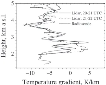
2
3
4
5
−
10
−
5
0
5
Temperature gradient, K/km
Height, km a.s.l.
Lidar, 20-21 UTC Lidar, 21-22 UTC Radiosonde
Fig. 12. Temperature gradients on 10 July 2006 of the lidar tem-perature profile measured between 20:00–21:00 UTC (1t=60 min) (see Fig. 9), the lidar profile number 5 (1t=6 min) from Fig. 11 and the radiosonde launched at 21:10 UTC.
shown in Figs. 13 and 14 in greater detail. The tempera-ture gradient in Fig. 14 corresponds to the gradient along the line of sight of the measurement. The air flowing against the mountain ridge is lifted up which causes a steep temper-ature gradient to the west (profile number 8 (see Fig. 10) at ranges around 1 km) in the direction of the measurement. Be-cause of a stable atmosphere, the rising warm air is blocked at around 1.5 km a.g.l. just atop Hornisgrinde. To the east, a se-quence of stable and more unstable regions developed. This can be seen in profile number 3 (see Fig. 10) in about 1 km and 2.2 km range as well as in profile number 2 in 2 km and 3 km range where the lowest temperature gradients are per-sisting bounded by stable layers. We believe that this shows gravity waves initiated at the mountain ridge.
7 Conclusions and outlook
We have developed a lidar for high-resolution rotational Ra-man temperature measurements at 355 nm. The receiver makes use of multicavity interference filters in a sequential setup. That way we gain very high efficiency when sepa-rating the signals and a high suppression of the elastically backscattered light in the rotational Raman channels. Fur-thermore, we are able to change the system’s sensitivity by selecting the tilting angles of the filters. We performed sim-ulations to optimize the filter parameters for RR tempera-ture measurements for both high nighttime and daytime per-formance in the lower troposphere. A noontime tempera-ture measurement resulted in uncertainties less than 1 K for ranges up to 1 km for 1 min integration time. The lidar al-lows to measure temperature fields by the use of a scanner. This gives a new tool to study, e.g. the highly complex
struc-0 -1 -2
-3 1 2 3
Horizontal Distance, km
1161 m, Lidar Site
→ Ε
W ←
←
270 290
280 285
275
T
, K
1 2 3
Hei
ght, km a
.s
.l
. 4
Wind direction
Fig. 13. Temperature field measured over Hornisgrinde on 10 July 2006 between 21:00–22:00 UTC (same profiles shown in Fig. 11). Lines mark the 285-K isotherm.
0 -1 -2
-3 1 2 3
1 2 3
Height, km a.s.l.
Horizontal Distance, km
1161 m, Lidar Site
→ Ε
W ←
4
←
-10 10
0 5
-5
dT/dR
, K/km
Fig. 14. Field of the temperature gradient along the line of sight calculated with the profiles shown in Fig. 11.
ture of the temperature field over mountainous terrain. In the example shown, an averaging of the individual lidar profiles over 6 min and a spatial averaging, ranging from 300 m to 1200 m, yields in measurement uncertainties of smaller than 1.1 K up to a range of 4 km. Temperature profiling cover-ing the whole troposphere up to 13 km altitude with statisti-cal temperature uncertainties of less than 1 K is demonstrated with 60 min integration time.
than 300 m within the boundary layer without any extra day-light filter and an accuracy of1T <1 K.
Acknowledgements. This research was supported within the Convective Storms Virtual Institute (COSI-TRACKS) of the German Helmholtz Association. The authors are grateful to GKSS, Geesthacht, Germany to donate the mobile platform, to the Institute for Tropospheric Research, Leipzig, Germany, for the supply of the laser and to the National Center for Atmospheric Research, Boulder, CO for building the scanner and the technical support. Thanks to T. Schaberl for the interior fittings as well as to S. Pal for the support during the field campaigns.
Edited by: W. Ward
References
Arshinov, Y., Bobrovnikov, S., Serikov, I., Althausen, D., Ansmann, A., Mattis, I., M¨uller, D., and Wandinger, U.: Optic-fiber scram-blers and fourier transform lens as a means to tackle the problem on the overlap factor of lidar, Proceedings of the 22nd Interna-tional Laser Radar Conference, 227–230, 2004.
Arshinov, Y., Bobrovnikov, S., Serikov, I., Ansmann, A., Wandinger, U., Althausen, D., Mattis, I., and M¨uller, D.: Day-time operation of a pure rotational Raman lidar by use of a Fabry-Perot interferometer, Appl. Optics, 44, 3593–3603, 2005. Behrendt, A. and Reichardt, J.: Atmospheric temperature profiling
in the presence of clouds with a pure rotational Raman lidar by use of an interference-filter-based polychromator, Appl. Optics, 39, 1372–1378, 2000.
Behrendt, A.: Fernmessung atmosphrischer Temperaturprofile in Wolken mit Rotations-Raman-Lidar, doctoral dissertation (Uni-versity of Hamburg, Hamburg, Germany), 2000.
Behrendt, A., Nakamura, T., Onishi, M., Baumgart, R., and Tsuda, T.: Combined Raman lidar for the measurement of atmospheric temperature, water vapor, particle extinction coefficient, and par-ticle backscatter coefficient, Appl. Optics, 41, 7657–7666, 2002. Behrendt, A., Nakamura, T., Tsuda, T., and Wulfmeyer, V.: Rota-tional Raman temperature lidar: New experimental results and performance expected for future ground-based and airborne sys-tems, Proceedings of the 22nd International Laser Radar Confer-ence, 2004a.
Behrendt, A., Nakamura, T., and Tsuda, T.: Combined tempera-ture lidar for measurements in the troposphere, stratosphere, and mesosphere, Appl. Optics, 43, 2930–2939, 2004b.
Behrendt, A.: Temperature Measurements with Lidar, in: Lidar: Range-Resolved Optical Remote Sensing of the Atmosphere, edited by: Weitkamp, C., Springer, New York, 2005.
Cooney, J.: Measurement of atmospheric temperature profiles by Raman backscatter, Appl. Meteorol., 11, 108–112, 1972. Di Girolamo, P., Marchese, R., Whiteman, D. N., and
De-moz, B.: Rotational Raman Lidar measurements of atmo-spheric temperature in the UV, Geophys. Res. Lett., 31, L01106, doi:10.1029/2003GL018342, 2004.
Di Girolamo, P., Behrendt, A., and Wulfmeyer, V.: Spaceborne profiling of atmospheric temperature and particle extinction with pure rotational Raman lidar and of relative humidity in
combina-tion with differential absorpcombina-tion lidar: performance simulacombina-tions, Appl. Optics, 45, 2474–2494, 2006.
Hair, J. W., Caldwell, L. M., Krueger, D. A., and She, C. Y.: High-spectral-resolution lidar with iodine-vapor filters: measure-ment of atmospheric-state and aerosol profiles, Appl. Optics, 40, 5280–5294, 2001.
Hua, D., Uchida, M., and Kobayashi, T.: Ultraviolet Rayleigh-Mie lidar with Mie-scattering correction by Fabry-Perot etalons for temperature profiling of the troposphere, Appl. Optics, 44, 1305– 1314, 2005.
Hua, D., Uchida, M., and Kobayashi, T.: Ultraviolet Rayleigh-Mie lidar for daytime-temperature profiling of the troposphere, Appl. Optics, 44, 1315–1322, 2005.
Mattis, I., Ansmann, A., Althausen, D., Jaenisch, V., Wandinger, U., M¨uller, D., Arshinov, Y. F., Bobrovnikov, S. M., and Serikov, I. B.: Relativ-humidity profiling in the troposphere with a Raman lidar, Appl. Optics, 41, 6451–6462, 2002.
Nedeljkovic, D., Hauchecorne, A., and Chanin, M.-L.: Rota-tional Raman lidar to measure the atmospheric temperature from ground to 30 km, IEEE Trans. Geosci. Remote Sens., 31, 90–101, 1993.
Pety, D. and Turner, D.: Combined analog-to-digital and photon counting detection utilized for continous Raman lidar measure-ments, Proceedings of the 23rd International Laser Radar Con-ference, post deadline paper, 2006.
Shimizu, H., Lee, S. A., and She, C. Y.: High spectral resolution lidar system with atomic blocking filters for measuring atmo-spheric parameters, Appl. Optics, 22, 1373–1381, 1983. Schwiesow, R. L. and Lading, L.: Temperature profiling by
Rayleigh-scattering lidar, Appl. Optics, 20, 1972–1979, 1981. Spuler, S. and Mayor, S.: Scanning Eye-Safe Elastic Backscatter
Lidar at 1.54µm, J. Atmos. Ocean. Technol., 22, 696–703, 2005. Vaughan, G., Wareing, D. P., Pepler, S. J., Thomas, L., and Mitev, V. M.: Atmospheric temperature measurements made by rotational Raman scattering, Appl. Optics, 32, 2758–2764, 1993.
Whiteman, D. N., Demoz, B., Di Girolamo, P., Comer, J., Veselovskii, I., Evans, K., Wang, Z., Cadirola, M., Rush, K., Schwemmer, G., Gentry, B., Melfi, S. H., Mielke, B., Venable, D., and Van Hove, T.: Raman lidar measurements during the International H2O Project. Part I: Instrumentation and Analysis
Techniques, J. Atmos. Ocean. Tech., 23, 157–169, 2006. Zeyn, J., Lahmann, W., and Weitkamp, C.: Remote daytime