Separating mixtures of aerosol types in airborne High Spectral Resolution Lidar data

(1)

AMTD

6, 8269–8309, 2013

Aerosol mixtures in HSRL data

S. P. Burton et al.

Title Page

Abstract Introduction

Conclusions References

Tables Figures

◭ ◮

Back Close

Full Screen / Esc

Printer-friendly Version Interactive Discussion

Discussion

P

a

per

|

Dis

cussion

P

a

per

|

Discussion

P

a

per

|

Discussio

n

P

a

per

|

Atmos. Meas. Tech. Discuss., 6, 8269–8309, 2013 www.atmos-meas-tech-discuss.net/6/8269/2013/ doi:10.5194/amtd-6-8269-2013

Atmospheric Measurement

Techniques

Open Access

Discussions

Geoscientiic Geoscientiic

This discussion paper is/has been under review for the journal Atmospheric Measurement Techniques (AMT). Please refer to the corresponding final paper in AMT if available.

Separating mixtures of aerosol types in

airborne High Spectral Resolution Lidar

data

S. P. Burton, M. A. Vaughan, R. A. Ferrare, and C. A. Hostetler

NASA Langley Research Center, MS 475, Hampton, VA, 23681, USA

Received: 17 August 2013 – Accepted: 3 September 2013 – Published: 6 September 2013 Correspondence to: S. P. Burton (sharon.p.burton@nasa.gov)

(2)

AMTD

6, 8269–8309, 2013

S. P. Burton et al.

Title Page

Tables Figures

◭ ◮

Back Close

Full Screen / Esc

Discussion

P

a

per

|

Dis

cussion

P

a

per

|

Discussion

P

a

per

|

Discussio

n

P

a

per

|

Abstract

Knowledge of aerosol type is important for source attribution and for determining the magnitude and assessing the consequences of aerosol radiative forcing. However, at-mospheric aerosol is frequently not a single pure type, but instead occurs as a mixture of types, and this mixing a_ffects the optical and radiative properties of the aerosol. This

5

paper extends the work of earlier researchers by using the aerosol intensive param-eters measured by the NASA Langley Research Center airborne High Spectral Res-olution Lidar (HSRL-1) to develop a comprehensive and unified set of rules for char-acterizing the external mixing of several key aerosol intensive parameters: extinction-to-backscatter ratio (i.e. lidar ratio), backscatter color ratio, and depolarization ratio.

10

We present the mixing rules in a particularly simple form that leads easily to mixing rules for the covariance matrices that describe aerosol distributions, rather than just scalar values of measured parameters. These rules can be applied to infer mixing ratios from the lidar-observed aerosol parameters, even for cases without significant depolarization. We demonstrate our technique with measurement curtains from three

15

HSRL-1 flights which exhibit mixing between two aerosol types, urban pollution plus dust, marine plus dust, and smoke plus marine. For these cases, we infer a time-height cross-section of mixing ratio along the flight track, and partition aerosol extinction into portions attributed to the two pure types.

1 Introduction 20

Atmospheric aerosols play an important role in climate change and solar energy avail-ability and affect air quality and human health, but there are still significant uncertainties in our knowledge of the radiative e_ffects of aerosol (IPCC, 2007). The vertical distribu-tion of aerosol is particularly important, since aerosol lifetime and climate response depend on altitude (Hansen et al., 1997). Uniquely among remote sensing

measure-25

(3)

AMTD

6, 8269–8309, 2013

S. P. Burton et al.

Title Page

Tables Figures

◭ ◮

Back Close

Full Screen / Esc

Discussion

P

a

per

|

Dis

cussion

P

a

per

|

Discussion

P

a

per

|

Discussio

n

P

a

per

|

aerosol properties within the atmospheric column. At the same time, the determination of aerosol radiative forcing and source attribution also requires knowledge of aerosol type. Depending on the sophistication of the lidar instrument, one or more aerosol in-tensive parameters can be measured. Inin-tensive parameters are quantities that vary only with aerosol type and not amount and which can therefore be used for aerosol

5

classification (Burton et al., 2012). For the NASA Langley Research Center (LaRC) airborne High Spectral Resolution Lidar (HSRL-1) (Hair et al., 2008), these parameters include the depolarization ratio at 532 and 1064 nm, aerosol extinction to backscatter ratio (lidar ratio) at 532 nm, and the spectral ratio of aerosol backscatter (i.e. backscat-ter color ratio).

10

Observed aerosol layers are frequently mixtures of multiple types. For passive in-struments, which observe full columns rather than vertically resolved profiles, the mea-surements reflect an effective mix of aerosols throughout the column. The assumption of a single aerosol type throughout the column is also frequently required in retrievals of aerosol extinction from elastic backscatter lidar (even though the backscatter

mea-15

surements are vertically resolved) (Fernald, 1984). Standard retrievals for the Cloud-Aerosol Lidar with Orthogonal Polarization (CALIOP) lidar on the Cloud-Cloud-Aerosol Lidar and Infrared Pathfinder Satellite Observations (CALIPSO) satellite do not make this assumption; however, they do require significant layer averaging that can result in lay-ers that include multiple different aerosol types. In those cases, the effective lidar ratio

20

and other properties depend on multiple types, complicating the retrieval (Burton et al., 2013). Even in very highly resolved measurements, aerosols are often present in a mixed state (Tesche et al., 2009; Petzold et al., 2011). Mixing between aerosol types can be either external or internal. In external mixing, the aerosol particles are physically separated and individually pure. Composite particles formed by, for example,

coagu-25

lation or aqueous reactions are considered internal mixtures (Lesins et al., 2002). We focus on external mixtures in this paper.

(4)

AMTD

6, 8269–8309, 2013

S. P. Burton et al.

Title Page

Tables Figures

◭ ◮

Back Close

Full Screen / Esc

Discussion

P

a

per

|

Dis

cussion

P

a

per

|

Discussion

P

a

per

|

Discussio

n

P

a

per

|

include some mixtures, for example Polluted Dust in the CALIPSO aerosol classifica-tion (Omar et al., 2009) and Polluted Maritime and Dusty Mix in the NASA HSRL-1 classification (Burton et al., 2012). Groß et al. (2013) also address mixtures, by in-cluding mixing lines to indicate regions in the multi-dimensional measurement space representing mixtures between two types, either Saharan dust and marine aerosol or

5

Saharan dust and biomass-burning aerosol. These mixing line equations build on a heritage (including Groß et al., 2011; Gasteiger et al., 2011; Tesche et al., 2009) that dates back at least a decade. L ´eon et al. (2003) and Kaufman et al. (2003) used equa-tions for the inverse lidar ratio and backscatter angstrom exponent for a mixture of two modeled aerosol modes. Sugimoto et al. (2003) examined mixtures of dust and

non-10

dust aerosol and derived equations linking the depolarization with the partitioning of backscatter and, in later work, the backscatter-related Angstrom exponent (Sugimoto and Lee, 2006). While not explicitly providing equations for aerosol intensive proper-ties of mixtures, Nishizawa et al. (2010) do an extinction retrieval similar to that of L ´eon et al. (2003) but use both the depolarization ratio and spectral relationship of the

15

measured backscatter to choose between three specific aerosol models; they present results as partitions of aerosol extinction. In this paper, we infer mixing ratios and extinc-tion partiextinc-tions for various cases of mixing, including a non-dust case where we cannot rely on variation in the depolarization ratio to achieve the separation. We also expand on the equations of L ´eon et al. (2003) and Sugimoto and Lee (2006) by showing that,

20

with a fortuitous choice of variables, the mixing equations can all be recast in the form of linear combinations. This more convenient form then leads easily to a representation of the full variance-covariance matrices for mixtures of multivariate normal distributions as well.

The classification algorithms used by Groß et al. (2013) and Weinzierl et al. (2011)

25

(5)

AMTD

6, 8269–8309, 2013

S. P. Burton et al.

Title Page

Tables Figures

◭ ◮

Back Close

Full Screen / Esc

Discussion

P

a

per

|

Dis

cussion

P

a

per

|

Discussion

P

a

per

|

Discussio

n

P

a

per

|

distributions of aerosol types were calculated from the NASA Langley HSRL-1 (Burton et al., 2012) and are an important part of the aerosol classification methodology in use for that instrument. This article builds on the work of Burton et al. (2012) and shows mixtures of aerosol types in the framework of multivariate normal distributions using measurements from the NASA Langley airborne HSRL-1.

5

Following a brief instrument description in Sect. 2, Sect. 3 presents a derivation of the linear mixing equations for aerosol intensive parameters, expanding on the work in earlier papers. In Sect. 4, we extend the equations to include not just the mean values but also the full covariance matrix for a mixture of two multivariate normal distributions. In the second half of this paper, in Sects. 5–7, we will show three case studies of

10

external mixtures observed by the NASA Langley airborne HSRL-1, which satisfy the derived relationships. We also estimate mixing ratios for our case studies and show the apportionment of aerosol extinction to the two constituent types.

2 Instrument description

HSRL-1 (Hair et al., 2008) is the first airborne high spectral resolution lidar

instru-15

ment built and operated by NASA Langley Research Center. Between March 2006 and October 2012, HSRL-1 has flown more than 1200 h during 357 science flights on the NASA King Air B200 on twenty field campaigns across North America. The HSRL technique independently retrieves aerosol and tenuous cloud extinction and backscatter (Grund and Eloranta, 1991) without a priori information on aerosol type

20

or extinction-to-backscatter ratio, as is required for standard elastic backscatter lidar retrievals. The NASA HSRL-1 employs the HSRL technique at 532 nm and the stan-dard backscatter technique at 1064 nm. It also measures depolarization ratio at both wavelengths. HSRL-1 is well calibrated and has been extensively validated using in situ and remote sensing measurements; the HSRL-1 aerosol optical thickness (AOT)

25

(6)

AMTD

6, 8269–8309, 2013

S. P. Burton et al.

Title Page

Tables Figures

◭ ◮

Back Close

Full Screen / Esc

Discussion

P

a

per

|

Dis

cussion

P

a

per

|

Discussion

P

a

per

|

Discussio

n

P

a

per

|

direct and unambiguous retrieval of loading-invariant aerosol intensive properties in ad-dition to loading-dependent extensive properties such as AOT. The intensive properties provided by HSRL-1 are the 532 nm lidar ratio, the aerosol depolarization ratios at both 532 and 1064 nm, and the backscatter color ratio (i.e., the ratio of aerosol backscatter coe_fficients at the two wavelengths; the 1064-nm backscatter depends on a nominal

5

lidar ratio, but the systematic error this assumption produces does not greatly a_ffect the ratio used in aerosol classification, due to limited sensitivity of backscatter to the lidar ratio assumption at 1064 nm (Burton et al., 2012)). The intensive parameters provide information about the aerosol physical properties and are combined to infer aerosol type (Burton et al., 2012).

10

3 Mixing relationships

Analytically derived lidar observables for mixtures are discussed by Kaufman et al. (2003) and L ´eon et al. (2003), who derive backscatter-to-extinction ratio and a backscatter-related pseudo Angstrom exponent for a mixture of a fine and a coarse aerosol mode using Moderate Resolution Imaging Spectroradiometer (MODIS) aerosol

15

models. Their starting point is a simple partition of extinction,α, into fine and coarse modes with the fine mode fraction defined in terms of aerosol extinction.

f ≡ αs

α_s₊α_l (1)

Here, subscripts “s” and “l” indicate small and large mode. We are interested in the lidar ratio, or extinction-to-backscatter ratio, the inverse of the quantity used by L ´eon et

20

al. (2003). The pseudo Angstrom exponent they use likewise is related to the backscat-ter color ratio we use, but not identical. Also, we wish to mix two arbitrary aerosol types, which we will calla andb, not single modes. Therefore, we start our derivation from a slightly di_fferent point, with the goal of producing mixing ratio equations in a very sim-ple form. Nevertheless the mixing relations given here are consistent with those given

(7)

AMTD

6, 8269–8309, 2013

S. P. Burton et al.

Title Page

Tables Figures

◭ ◮

Back Close

Full Screen / Esc

Discussion

P

a

per

|

Dis

cussion

P

a

per

|

Discussion

P

a

per

|

Discussio

n

P

a

per

|

by earlier authors, and we will show how to convert between them later in this section (Eq. 20).

We start with a mixing ratio (partition) defined in terms of aerosol backscatter

p≡ βa

β_a₊β_b (2)

where β denotes aerosol backscatter coe_fficient, and subscripts “a” and “b” denote

5

the contributions from two types. First, the aerosol backscatter component of each constituent type can be written in terms of the partition and the backscatter of the mixture:

β_a₌pβ (3)

10

β_b₌(1−p)β (4)

Then, to represent the aerosol extinction, α, for the constituent types, we apply the aerosol extinction-to-backscatter ratio, or lidar ratio,S.

α_a₌S_aβ_a₌S_apβ (5)

15

α_b₌S_bβ_b₌S_b(1−p)β (6)

We note that the aerosol lidar ratio is typically represented asS_a with a subscript “a” for “aerosol”. In this work, however, we drop this customary subscript to avoid confus-ing it with the subscripts “a” and “b” indicatconfus-ing specific aerosol types. All lidar ratios, depolarization ratios, and backscatter and extinction coefficients in this paper should

20

(8)

AMTD

6, 8269–8309, 2013

S. P. Burton et al.

Title Page

Tables Figures

◭ ◮

Back Close

Full Screen / Esc

Discussion

P

a

per

|

Dis

cussion

P

a

per

|

Discussion

P

a

per

|

Discussio

n

P

a

per

|

With the definitions of aerosol extinction and backscatter for the two types given in Eqs. (3)–(6), we can proceed to deriving the lidar ratio of the mixture. The lidar ratio is the ratio of aerosol extinction to aerosol backscatter coe_fficient.

S₌α

β (7)

Inserting Eqs. (5) and (6) in the numerator,

5

=

S_ap₊S_b(1−p)

β

β (8)

Cancelling terms in the numerator and denominator leaves a simple expression for the lidar ratio of the mixture in terms of a linear combination of the lidar ratio of each of the two constituent types.

S₌S_ap₊S_b(1−p) (9)

10

This relationship is true at any wavelength, but both the lidar ratios and the mixing ratio

p are wavelength dependent. We must therefore derive the wavelength dependence of the mixing parameter. Accordingly, we will introduce a superscriptλto indicate the wavelength dependence of the mixing ratio and other quantities and write Eq. (2) more explicitly for the 1064 nm channel.

15

p₁₀₆₄₌ β

1064 a

β_a1064₊β1064

b

(10)

To get the relationships between channels, we need the backscatter color ratio

χ₌ β

532

(9)

AMTD

6, 8269–8309, 2013

S. P. Burton et al.

Title Page

Tables Figures

◭ ◮

Back Close

Full Screen / Esc

Discussion

P

a

per

|

Dis

cussion

P

a

per

|

Discussion

P

a

per

|

Discussio

n

P

a

per

|

The color ratios for the two pure types will be indicated byχ_aandχ_b. The mixing ratio at 532 nm is derived following similar steps.

p₅₃₂₌ β

532 a

β532_a ₊β532

b

(12)

= χaβ

1064 a

χ_aβ_a1064₊χ_bβ1064

b

(13)

5

Combining with Eqs. (3) and (4) and cancelling out the total aerosol backscatter in the numerator and denominator, we are left with the following equation, which gives the wavelength dependence of the mixing parameter. As long as the mixing ratio is known at one wavelength, along with color ratio values for the two pure types, the mixing ratio at other wavelengths can be obtained.

10

p₅₃₂₌ χap1064

χ_ap₁₀₆₄₊χ_b(1−p₁₀₆₄) (14)

We can write the equation for the lidar ratio at 532 nm as a linear combination of the 532 nm lidar ratios of each pure type like this:

S532₌S_a532p₅₃₂₊S_b532(1−p₅₃₂) (15)

or like this:

15

S532₌S

532

a χap1064+S

532

b χb(1−p1064)

χ_ap₁₀₆₄₊χ_b(1−p₁₀₆₄) (16)

(10)

AMTD

6, 8269–8309, 2013

S. P. Burton et al.

Title Page

Tables Figures

◭ ◮

Back Close

Full Screen / Esc

Discussion

P

a

per

|

Dis

cussion

P

a

per

|

Discussion

P

a

per

|

Discussio

n

P

a

per

|

ratio itself.

χ₌χaβ

1064

a +χbβ1064b

β1064_a ₊β1064

b

(17)

χ₌

χ_ap₁₀₆₄₊χ_b(1−p₁₀₆₄)

β1064

β1064 (18)

5

χ₌χ_ap₁₀₆₄₊χ_b(1−p₁₀₆₄) (19)

So this also mixes linearly. That is, the form of the equation is the same as Eq. (9) and furthermore the mixing parameter is the same as for the lidar ratio at 1064 nm.

A similar derivation yields the relationship between the backscatter partition p_λ at any wavelength and the partition of extinction,f_λ, that was defined in Eq. (1).

10

f_λ₌ S

λ

apλ

S_aλp_λ₊Sλ

b(1−pλ)

(20)

The final intensive parameter that we use for aerosol classification is the aerosol depo-larization ratio. Following the same logic as Sugimoto and Lee (2006), it is possible to derive the aerosol depolarization ratio of a mixture. Multiple definitions of depolariza-tion ratio are in use (Cairo et al., 1999; Gimmestad, 2008), and we must be specific.

15

We consider only the depolarization due to aerosols, and, using the same notation as Sugimoto and Lee (2006), we use the symbolδ for the ratio of the aerosol backscat-ter coe_fficient measured in the perpendicular channel to that measured in the parallel channel,

δ₌β⊥

β_k (21)

(11)

AMTD

6, 8269–8309, 2013

S. P. Burton et al.

Title Page

Tables Figures

◭ ◮

Back Close

Full Screen / Esc

Discussion

P

a

per

|

Dis

cussion

P

a

per

|

Discussion

P

a

per

|

Discussio

n

P

a

per

|

and the symbolδ′for the ratio of perpendicular to total aerosol backscatter.

δ′₌ β⊥

β_k₊β_⊥ (22)

δ′₌ δ

1+δ (23)

Note that the second half of Sugimoto and Lee’s (2006) Eq. (3) relating the two

depo-5

larization parameters includes a typographical error. It should be this:

δ₌ δ

′

1−δ′ (24)

Aerosol depolarization measurements from lidar are usually reported as defined by Eq. (21) . This includes archived aerosol depolarization ratio measurements from the NASA airborne HSRL-1 used in this study and by Burton et al. (2012). However, for

10

the mixing equations in this study, we will use δ′ from Eq. (22) because this is the quantity that mixes linearly. To distinguish between them more conveniently, we will use the term “aerosol depolarization potential” for the quantityδ′and the term “aerosol depolarization ratio” for the more familiar quantity,δ. The term “depolarization potential” is inspired by Gimmestad (2008) who describes it as “a measure of the propensity of

15

the scattering medium to depolarize the incident polarization.”

Sugimoto and Lee (2006) use the backscatter mixing ratio, which they call X, and we callp₅₃₂. Without assuming that one type is totally non-depolarizing as they do, we can write a more general form of their Eq. (6) for two types. Sugimoto and Lee’s equation relates the depolarization ratio, δ, of a mixture to the depolarization potential, δ′, of

20

(12)

AMTD

6, 8269–8309, 2013

S. P. Burton et al.

Title Page

Tables Figures

◭ ◮

Back Close

Full Screen / Esc

Discussion

P

a

per

|

Dis

cussion

P

a

per

|

Discussion

P

a

per

|

Discussio

n

P

a

per

|

more useful for our later development in Sect. 4.

δ′mix₅₃₂

1−δ′mix 532

= δ

′

ap532+δ

′

b(1−p532)

(1−δ′

a)p532+(1−δ′b) (1−p532)

(25)

Invert and add 1 to both sides:

1

δ′mix 532

= 1−δ

′ a

p₅₃₂₊ 1−δ′_b

(1−p₅₃₂)

δ′

ap532+δ′b(1−p532)

+δ

′

ap532+δ′b(1−p532)

δ′

ap532+δ′b(1−p532)

(26)

Canceling terms in the numerator and inverting again yields

5

δ′mix₅₃₂₌δ′_ap₅₃₂₊δ′_b(1−p₅₃₂) (27)

Not only is this in the convenient form of a linear combination, but the mixing ratio is the same as the 532 nm backscatter mixing ratio found in Eq. (15).

4 Multivariate normal distributions for mixture types

The previous section provides mixing rules for the mean values of lidar intensive

pa-10

rameters. However, as discussed in the introduction, for some applications it is useful to examine not just mean values, but also to estimate model distributions for the mixtures. Burton et al. (2012) use multivariate normal distributions for various aerosol types, in-cluding both pure types and some mixtures, which were based on HSRL measure-ments of various types. However, the mixtures included in this scheme were based

15

empirically on specific mixture cases that were straightforward to identify in HSRL-1 observations. Here, we analytically calculate the multivariate normal distributions of a mixture, given covariance matrices describing distributions for two pure types. Recall that the set of normal distributions is closed under linear transformations. Therefore, the equations in Sect. 3 showing lidar-observed aerosol intensive parameters in the

(13)

AMTD

6, 8269–8309, 2013

S. P. Burton et al.

Title Page

Tables Figures

◭ ◮

Back Close

Full Screen / Esc

Discussion

P

a

per

|

Dis

cussion

P

a

per

|

Discussion

P

a

per

|

Discussio

n

P

a

per

|

form of linear combinations are in a particularly convenient form. Following Burton et al. (2012) and earlier authors (Cattrall et al., 2005), we assume that the lidar measure-ments for pure types can be approximated by multivariate normal distributions; in that case, the linear equations imply that a mixture of two pure types with a specific mixing ratio can also be approximated as a multivariate normal distribution.

5

Specifically, given that an optical measurement of depolarization potential, lidar ratio, or color ratio – written generically byx_mix– can be represented as a linear combination of two pure types as given in Sect. 3,

x_mix₌px_a₊(1−p)x_b (28)

then we define measurement vectorsAandBcomprising those three quantities for the

10

two pure types, “a” and “b”.

A=



 

δ_a′532

S532_a

χ_a





 B=



 

δ_b′532

S532_b

χ_b





 (29)

The vectorX that describes the mixture is given by the vector equation

X=PA+(I−P)B (30)

whereIis the identity matrix andPis a diagonal matrix composed of the mixing ratios

15

for each measurement dimension.

P= 



p₁ 0 0 0 p₂ 0 0 0 p₃



=



 

χ_ap₁₀₆₄

χ_ap1064+χ_b(1−p₁₀₆₄) 0 0

0 χap1064

χ_ap1064+χ_b(1−p₁₀₆₄) 0

0 0 p₁₀₆₄





 (31)

(14)

AMTD

6, 8269–8309, 2013

S. P. Burton et al.

Title Page

Tables Figures

◭ ◮

Back Close

Full Screen / Esc

Discussion

P

a

per

|

Dis

cussion

P

a

per

|

Discussion

P

a

per

|

Discussio

n

P

a

per

|

by covariance matricesΣX,ΣA andΣB then, the covariance matrix for the mixing state

Xis given as follows (Parois and Lutz, 2011),

ΣX =PΣAPt+(I−P)ΣB(I−P)t (32)

where superscript t indicates the transpose operation. Recall that the diagonal ele-ments of the covariance matrix are the variances, while the off-diagonal elements are

5

the covariance terms:

Σ = 

  

σ₁2 ρ₁₂σ₁σ₂ ρ₁₃σ₁σ₃

ρ₁₂σ₁σ₂ σ₂2 ρ₂₃σ₂σ₃

ρ₁₃σ₁σ₃ ρ₂₃σ₂σ₃ σ₃2



  

(33)

Writing out the diagonal terms of Eq. (32) produces the familiar propagation of errors for a linear combination (e.g. Bevington and Robinson, 1992).

σ_{X i}2 ₌p2_iσ_Ai2₊(1−p_i)2σ_Bi2 for i ₌δ₅₃₂′ , S₅₃₂, χ (34)

10

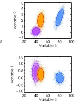
Equation (32) can be illustrated by simulation, as shown in Fig. 1. Here two covariance matrices are arbitrarily selected to represent pure types. Points randomly selected from these distributions are shown in blue and purple. Blue and purple ellipses show the 2-sigma contours of the covariance matrices for the pure types (when representing covariance matrices as ellipses, the major and minor axes are given by the square root

15

of the eigenvalues while the directions are determined by the eigenvectors (Rodgers, 2000)). A specific mixture of the two pure types is calculated numerically by mixing the blue and purple points using three different mixing ratios for the three dimensions, and these points are shown in orange. The mixing ratios are (0.6, 0.2, 0.8). That is, Variable 1 is calculated as 60 % purple plus 40 % blue, Variable 2 is 20 % purple plus 80 % blue,

20

(15)

AMTD

6, 8269–8309, 2013

S. P. Burton et al.

Title Page

Tables Figures

◭ ◮

Back Close

Full Screen / Esc

Discussion

P

a

per

|

Dis

cussion

P

a

per

|

Discussion

P

a

per

|

Discussio

n

P

a

per

|

projection. Since the orange points are calculated numerically and the red ellipses are calculated analytically, and they agree, this simulation provides a demonstration that the form of the equation is correct.

5 HSRL-1 observations of dust and pollution mixtures during MILAGRO

HSRL-1 data from the MILAGRO (Megacity Initiative: Local and Global Research

Ob-5

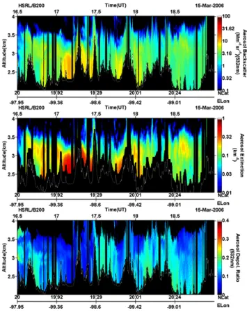
servations) campaign provide a further illustration of Eqs. (30) and (32). Figure 2 shows the aerosol backscatter coefficient, aerosol extinction coefficient and aerosol depolar-ization ratio at 532 nm for a flight in and around Mexico City on 15 March 2006. More details about the meteorological context and aerosol sources and transport in this case study are given by de Foy et al. (2011), who discuss comparisons of the Weather

10

Research and Forecasting (WRF)-Flexpart aerosol transport model and the HSRL-1 measurements for this case. Enhancements of backscatter and extinction in the data curtains mostly indicate urban aerosol from the Mexico City Metropolitan Area. The aerosol depolarization ratio, which is an indicator of non-spherical particles, is elevated throughout much of the boundary layer, indicating the influence of locally generated

15

dust.

Most of the scene consists of varying amounts of dust and pollution. While de Foy et al. (2011) also show a significant amount of fresh smoke in the region, here we limit the analysis to the region below 4 km above mean sea level (ASL) and no smoke plumes are included. Figure 3 shows the measurements on 15 March 2006 from HSRL-1 of

20

three intensive variables for all data points below 4 km having extinction in excess of 0.05 km−1. Here, the aerosol depolarization ratio has been converted to depolarization potential, since this is the quantity that mixes linearly, according to Eq. (27). Note that the intensive variables are spread over a continuum in all three measurement dimen-sions, supporting the inference of an external mixture between two types.

25

(16)

AMTD

6, 8269–8309, 2013

S. P. Burton et al.

Title Page

Tables Figures

◭ ◮

Back Close

Full Screen / Esc

Discussion

P

a

per

|

Dis

cussion

P

a

per

|

Discussion

P

a

per

|

Discussio

n

P

a

per

|

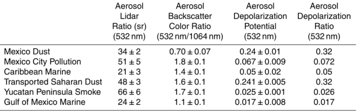
scene-specific measurements, rather than using generic models. For pure dust, we take an HSRL-1 measurement sample of locally generated dust from a dust plume ob-served on the slope of Pico de Orizaba, 200 km east of Mexico City, three days earlier on 12 March (de Foy et al., 2011). The 532 nm lidar ratio of this measurement sample, 34±2 sr, is smaller than typical values reported for Saharan dust close to the source

5

(Freudenthaler et al., 2009), but the high depolarization ratio, 0.32, is comparable to the values of 0.27–0.35 measured by Freudenthaler et al. (2009), suggesting this sam-ple is indeed pure dust, though of a di_fferent composition than Saharan dust. The very low backscatter color ratio (532 nm/1064 nm) of 0.70±0.07 indicates large particles. Again, these values differ from other HSRL-1 measurements of pure dust which mostly

10

correspond to transported Saharan dust (Burton et al., 2012). The smaller color ratios in this observation of dust in Mexico, directly at the source, probably imply the presence of large particles that have not yet deposited out of the plume. For this analysis, we also sample Mexico City urban pollution using the HSRL-1 aerosol classification mask (Bur-ton et al., 2012) from an overpass directly over Mexico City where the backscattering

15

and extinction are at a maximum. In contrast to the dust, this sample has a higher lidar ratio, 51±5 sr, larger backscatter color ratio, 1.8±0.1, and small depolarization ratio of 0.07, consistent with urban aerosol. These measurements are also shown in Table 1.

Numerically calculating the variance-covariance matrices for the pure-type measure-ment samples is straightforward. The ellipses representing the 2-sigma covariance

con-20

tours of the samples of pure dust and pure urban aerosol are shown in red in Fig. 3. Also shown, in orange, are ellipses representing covariance matrices for mixtures built using Eqs. (30)–(32) with mixing ratiosp₅₃₂ of 10, 20, 30. . . 90 %. The agreement be-tween the measured data and the envelope of the string of ellipses can be taken as confirmation of the derivations in Sects. 3 and 4 and an indicator that the aerosol in

25

this case is well represented as an external mixture.

(17)

AMTD

6, 8269–8309, 2013

S. P. Burton et al.

Title Page

Tables Figures

◭ ◮

Back Close

Full Screen / Esc

Discussion

P

a

per

|

Dis

cussion

P

a

per

|

Discussion

P

a

per

|

Discussio

n

P

a

per

|

mixing ratio at each point. But to infer a mixing ratio simultaneously consistent with all three measured variables, we instead use the calculated distributions for the mixtures il-lustrated in Fig. 3. For each point, we choose the mixing ratio by using the Mahalanobis distance to select which mixture distribution is the best fit to the three variables. The Mahalanobis distance (Mahalanobis, 1936), discussed in detail by Burton et al. (2012),

5

is a generalized metric that describes the “distance” between a measurement point and a multivariate normal distribution. For the examples discussed here, the mixing ratio is chosen to the nearest 10 % by minimizing the Mahalanobis distance with re-spect to each of the covariance matrices calculated by Eqs. (30)–(32) forp₅₃₂₌0, 10, 20,. . . 100 %. Figure 4 shows a time-height cross-section of the inferred mixing ratio,

10

p₅₃₂, for this flight.

Vertical lines in Fig. 4 indicate the point of closest approach to the MILAGRO cam-paign’s three measurement ground sites, T0, T1, and T2. In each case, the closest approach was within 10 km and 15 min of an Aerosol Robotic Network (AERONET) (Holben et al., 1998) observation. AERONET retrievals of coarse mode fraction (O’Neill

15

et al., 2003) at these locations and times were 4, 31, and 43 % for T0, T1, and T2, re-spectively. Assuming the dust in this scene is predominantly coarse mode, then the inferred dust mixing ratio in Fig. 4 for these three locations is in good agreement with these column values. For T0, the mixing ratio contour inferred for every point in the column was 0 %. At T1, most of the column falls on the 30 % mixing ratio contour, and

20

at T2, most of the column falls on the 40 % contour. However, Fig. 4 clearly shows in other parts of the scene, for example between 16:30 UT and 17:00 UT and again between 18:30–18:45, that there is significant vertical variability in the aerosol mixing ratio. These vertical gradients cannot be captured by a passive instrument that retrieves only column-equivalent values.

25

(18)

AMTD

6, 8269–8309, 2013

S. P. Burton et al.

Title Page

Tables Figures

◭ ◮

Back Close

Full Screen / Esc

Discussion

P

a

per

|

Dis

cussion

P

a

per

|

Discussion

P

a

per

|

Discussio

n

P

a

per

|

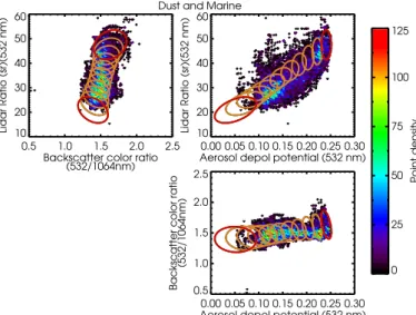
6 HSRL-1 observations of dust and marine mixtures in the Caribbean Sea

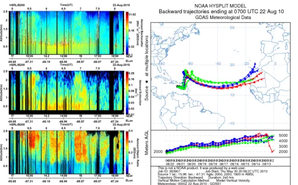
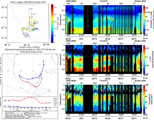
Another case of HSRL-1 observations of mixtures is shown in Fig. 6. On six days be-tween 18 August and 27 August 2010, HSRL-1 observed dust in the Caribbean trans-ported from Africa. Some of these cases are discussed by Burton et al. (2012, 2013). The observations shown in Fig. 6 occurred on 22 August south of Puerto Rico at 13◦–

5

19◦N latitude and 65◦–69◦W longitude. Back-trajectories calculated using the online Hybrid Single Particle Lagrangian Integrated Trajectory (HYSPLIT) tool from the NOAA Air Resources Laboratory READY website (http://ready.arl.noaa.gov/HYSPLIT.php) (Draxler and Rolph, 2013) lead back to Saharan Africa approximately 10 days earlier. In this scene, the main part of the dust layer is at relatively low altitude, in contact with

10

the marine boundary layer and mixing with it. This is evidenced by the depolarization-ratio curtain in Fig. 6, where the aerosol depolarization depolarization-ratio exceeds 0.10 even in the marine boundary layer. The aerosol intensive parameters are shown in Fig. 7 for all measurements with extinction above 0.05 km−1 (again, aerosol depolarization ratio is converted to aerosol depolarization potential for Fig. 7). To analyze these

measure-15

ments in terms of mixtures of dust plus marine aerosol, a pure dust sample was se-lected using the HSRL classification (Burton et al., 2012) from the part of this scene with the highest depolarization ratio, between 05:24 UT (5.4 UT) and 05:48 UT (5.8 UT) and between 1.4 and 2.4 km a.s.l. The measured depolarization ratio of this sample is again approximately 0.32 (which is 0.24 depolarization potential), the lidar ratio is

20

48±3 sr and the backscatter color ratio is 1.6±0.1 (see Table 1). The depolarization ratio is again consistent with pure dust; however, the larger backscatter color ratio in-dicates a smaller mean particle size, smaller than the locally generated Mexican dust discussed in Sect. 5. This is consistent with the largest particles being lost to depo-sition during transport. Aerosol depolarization ratio measurements greater than 0.10

25

(19)

AMTD

6, 8269–8309, 2013

S. P. Burton et al.

Title Page

Tables Figures

◭ ◮

Back Close

Full Screen / Esc

Discussion

P

a

per

|

Dis

cussion

P

a

per

|

Discussion

P

a

per

|

Discussio

n

P

a

per

|

are given in Table 1. The covariance matrices derived from the two samples of pure types are shown as red ellipses (2-sigma covariance) in Fig. 7.

Once again, the HSRL-1 measurements lie on a continuum between the two pure types and are in good agreement with the ellipses representing mixture covariance types from Eqs. (30)–(32). Note however that there is a significant di_fference in lidar

5

ratio and backscatter color ratio between the pure dust samples from the Mexico scene and the Caribbean scene. Other researchers (Esselborn et al., 2009; Schuster et al., 2012) have found that the lidar ratio for dust depends on source region, and that the size distribution changes as large particles are removed during transport (Maring et al., 2003; Weinzierl et al., 2011). The accuracy of the mixing ratio and partitioning results

10

depends on the accuracy of the models used. If the pure dust sample from Mexico City were used in place of the Caribbean dust model in this scene, the ellipses would not line up well with the data. For some applications, generic aerosol models may be unavoidable, but such models would be expected to produce only approximate results for the mixed states. Further study is required to determine how to best use generic

15

models for specific applications.

Figure 8 shows the inferred mixing ratio for this scene as a percentage of 532 nm backscatter due to dust and shows the partitioning of extinction for this scene. The marine aerosol is confined to the boundary layer. While most of the aerosol extinction due to dust is in a lofted layer, there is a significant amount of dust aerosol also in the

20

marine boundary layer, as expected.

7 HSRL-1 observations of mixed smoke and marine aerosol in the Gulf of Mexico

Our final case study occurred in the Gulf of Mexico near Veracruz on 28 March 2006, also during the MILAGRO field campaign. Figure 9 shows HSRL-1 measurement

cur-25

(20)

AMTD

6, 8269–8309, 2013

S. P. Burton et al.

Title Page

Tables Figures

◭ ◮

Back Close

Full Screen / Esc

Discussion

P

a

per

|

Dis

cussion

P

a

per

|

Discussion

P

a

per

|

Discussio

n

P

a

per

|

aerosol with low lidar ratios near 24 sr. The upper layer, from an airmass which crossed the Yucatan peninsula 24–48 h before the time of observation, has higher lidar ratios of 60–70 sr consistent with pollution or smoke. Figure 10 shows the aerosol lidar ratio and backscatter color ratio for measurements below 2500 m a.s.l. and having extinction greater than 0.05 km−1. The backscatter color ratio increases with lidar ratio such that

5

larger particles are associated with the lower lidar ratios (marine) and smaller particles are associated with higher lidar ratios (smoke or pollution). Considering the prevalence of small fires in the region (Fast et al., 2007), the airmass is probably best described as smoke aerosol. Both Figs. 9 and 10 show that the marine and smoke aerosol types are not cleanly separated. At altitudes in the middle of the boundary layer, the lidar

10

ratio and backscatter color ratio take on intermediate values. This suggests that there is mixing between the two types.

There is no dust in this scene and insignificant aerosol depolarization. Therefore the technique of Sugimoto and Lee (2006) and Tesche et al. (2009) for separating aerosol into dust and non-dust components would not be applicable in this case. In contrast,

15

the generalized technique presented in this study uses multiple aerosol intensive pa-rameters and does not require measurable depolarization. We therefore performed our separation technique for this case using only the lidar ratio and backscatter color ratio shown in Fig. 10. The covariance matrices for the pure types were both taken from measurement samples in this flight. The smoke sample is taken from between 1.5

20

and 2.0 km a.s.l. from the start of the flight before 14:28 UT (14.46 UT) where elevated aerosol extinction levels indicate higher aerosol loading. The marine sample was ob-tained below 0.7 km a.s.l. between 14:48 UT (14.8 UT) and 15:12 UT (15.2 UT) where the lidar ratio is low and has relatively little variability. The inferred mixing ratio and par-tition of extinction are shown in Fig. 11. As expected, most of the extinction in the lower

25

(21)

AMTD

6, 8269–8309, 2013

S. P. Burton et al.

Title Page

Tables Figures

◭ ◮

Back Close

Full Screen / Esc

Discussion

P

a

per

|

Dis

cussion

P

a

per

|

Discussion

P

a

per

|

Discussio

n

P

a

per

|

8 Summary and outlook

In summary, we show that lidar observable aerosol intensive parameters frequently re-flect mixtures between different aerosol types. We expand the derivations of equations used by previous researchers to describe external mixtures. The equations for each ob-servable can be written in the form of a linear combination of pure types, which allows

5

a mathematical description of mixture distributions rather than just scalar values. We also give the relationships between the mixing ratios for di_fferent intensive quantities at different wavelengths.

It’s important to acknowledge that not all variability in aerosol is due to external mix-ing. Humidification of aerosol (Su et al., 2008; Ferrare et al., 2001; Howell et al., 2006),

10

aging and deposition during transport (Maring et al., 2003; Weinzierl et al., 2011), and internal mixing (Lesins et al., 2002; Mishchenko et al., 2012) are other mechanisms that a_ffect aerosol intensive parameters, in ways which may not conform to the relationships presented here. However, we show three example flights where good agreement be-tween the lidar measurements and the analytical relationships support the assumption

15

of external mixing: of pollution plus dust, dust plus marine, and smoke plus marine. We also apply the equations to infer time-height cross-sections of mixing ratio and par-titions of extinction, which is possible even for cases which do not include dust (and therefore which have insignificant depolarization).

Unlike most passive instruments which give only total column amounts of

aerosol-20

relevant measurements, lidar measurements are fully resolved vertically. The ability to quantitatively apportion aerosol extinction to type in a vertically resolved measure-ment has the potential to greatly increase the information content that can be used for comparison and validation of global aerosol models and chemical transport models. Climate models are the usual means of assessing the impact of aerosol on climate and

25

(22)

AMTD

6, 8269–8309, 2013

S. P. Burton et al.

Title Page

Tables Figures

◭ ◮

Back Close

Full Screen / Esc

Discussion

P

a

per

|

Dis

cussion

P

a

per

|

Discussion

P

a

per

|

Discussio

n

P

a

per

|

(Textor et al., 2007). The aerosol classification from the NASA Langley airborne HSRL has previously been used to help evaluate and interpret aerosol models (e.g. de Foy et al., 2011). The ability to handle mixtures of aerosol types can potentially increase the usefulness of such comparisons, by providing more precise information on the vertical apportionment of aerosol by type. For example, using the standard HSRL-1 aerosol

5

classification (Burton et al., 2012), most of the Caribbean scene illustrated in Figs. 6–8 is classified qualitatively as “dusty mix”. The ability to quantify the amount of extinction in the marine boundary layer which is due to dust can give information on the deposi-tion of aerosol which can improve our understanding of aerosol transformadeposi-tion during transport and relates to measurements of primary productivity in the ocean.

10

Applications relating to climate science can be challenging for aircraft measure-ments, which are necessarily limited in time and space. However, the work presented suggests that a 2β₊1α₊2δ HSRL instrument (that is, an instrument with backscat-ter, extinction, and depolarization channels similar to the airborne HSRL-1) on a space platform could be used to quantitatively partition extinction by type in cases of external

15

mixing on a global basis. Such an instrument is possible with today’s technology, and could have a significant potential for furthering our current understanding of climate through improvements to and validation of global models.

The CALIPSO satellite lidar has provided global, vertically resolved measurements of aerosol from space since 2006. However, due to its smaller number of

measure-20

ment channels, aerosol extinction cannot be calculated without external information or assumptions. Some methods for providing more accurate aerosol extinction profiles from CALIPSO use column aerosol optical thickness as a constraint (e.g. Josset et al., 2010; Burton et al., 2010). This technique avoids the need to infer a lidar ratio but does still require the assumption of a uniform aerosol mixture throughout the column.

25

Calculations of mixtures from coincident HSRL-1 measurements on validation flights could potentially be used to help assess where and when this assumption is valid.

(23)

in-AMTD

6, 8269–8309, 2013

S. P. Burton et al.

Title Page

Tables Figures

◭ ◮

Back Close

Full Screen / Esc

Discussion

P

a

per

|

Dis

cussion

P

a

per

|

Discussion

P

a

per

|

Discussio

n

P

a

per

|

strument, HSRL-2, which makes measurements of extinction, backscatter, and de-polarization at 355 nm in addition to the measurements made by HSRL-1. The extra aerosol parameters from the airborne or a future spaceborne lidar with this capabil-ity are expected to improve the accuracy of aerosol mixing ratio estimates. Moreover, the second wavelength of extinction and backscatter measurements enables advanced

5

microphysical retrievals (M ¨uller et al., 1999), and the methods described here can im-prove those retrievals. The large search space of these microphysical retrievals can be constrained by quantitative calculations of aerosol partitioning from the much sim-pler calculations presented in this paper, potentially making them both faster and more accurate (Veselovskii et al., 2013). We plan to explore this combination of techniques

10

using data from the HSRL-2 instrument from past and future campaigns.

Finally, we note that altitude resolved aerosol mixing ratio from a spaceborne lidar similar to HSRL-1 or HSRL-2 could prove useful as a constraint for retrievals from coincident radiometer or, in particular, multi-angle polarimeter measurements. Such a combination of instruments is indeed called for on NASA’s ACE mission and we

antici-15

pate exploring joint lidar-polarimeter retrieval approaches using data from the airborne HSRL instruments and coincidently acquired polarimeter data from past and future field campaigns.

Acknowledgements. Funding for this research came from the NASA HQ Science Mission Di-rectorate Radiation Sciences Program and the NASA CALIPSO project. The authors also

ac-20

knowledge the NOAA Air Resources Laboratory (ARL) for the provision of the HYSPLIT trans-port and dispersion model and READY website (http://www.arl.noaa.gov/ready.php) used for some of the analysis described in this presentation, and we thank Brent Holben for establishing and maintaining the AERONET stations at the MILAGRO ground sites. Credit is owed to Cindy Brewer for the red-yellow-blue color set used in the mixing ratio plots. The authors are also very

25

(24)

AMTD

6, 8269–8309, 2013

S. P. Burton et al.

Title Page

Tables Figures

◭ ◮

Back Close

Full Screen / Esc

Discussion

P

a

per

|

Dis

cussion

P

a

per

|

Discussion

P

a

per

|

Discussio

n

P

a

per

|

Finally, we would like to thank Brian Cairns (NASA GISS) and Larry Thomason (NASA LaRC) for helpful discussions about the derivations presented in this paper.

References

Bevington, P. R. and Robinson, D. K.: Data Reduction and Error Analysis for the Physical Sci-ences, 2nd Ed., McGraw-Hill Inc., 328 pp., 1992.

5

Burton, S. P., Ferrare, R. A., Hostetler, C. A., Hair, J. W., Kittaka, C., Vaughan, M. A., Obland, M. D., Rogers, R. R., Cook, A. L., Harper, D. B., and Remer, L. A.: Using airborne high spectral resolution lidar data to evaluate combined active plus passive retrievals of aerosol extinction profiles, J. Geophys. Res.-Atmos., 115, D00H15, doi:10.1029/2009jd012130, 2010.

Burton, S. P., Ferrare, R. A., Hostetler, C. A., Hair, J. W., Rogers, R. R., Obland, M. D., Butler,

10

C. F., Cook, A. L., Harper, D. B., and Froyd, K. D.: Aerosol Classification of Airborne High Spectral Resolution Lidar Measurements – Methodology and Examples, Atmos. Meas. Tech., 5, 73–98, doi:10.5194/amt-5-73-2012, 2012.

Burton, S. P., Ferrare, R. A., Vaughan, M. A., Omar, A. H., Rogers, R. R., Hostetler, C. A., and Hair, J. W.: Aerosol classification from airborne HSRL and comparisons with the CALIPSO

15

vertical feature mask, Atmos. Meas. Tech., 6, 1397–1412, doi:10.5194/amt-6-1397-2013, 2013.

Cairo, F., Di Donfrancesco, G., Adriani, A., Pulvirenti, L., and Fierli, F.: Comparison of Various Linear Depolarization Parameters Measured by Lidar, Appl. Opt., 38, 4425–4432, 1999. Cattrall, C., Reagan, J., Thome, K., and Dubovik, O.: Variability of aerosol and spectral lidar and

20

backscatter and extinction ratios of key aerosol types derived from selected Aerosol Robotic Network locations, J. Geophys. Res.-Atmos., 110, D10S11, doi:10.1029/2004jd005124, 2005.

de Foy, B., Burton, S. P., Ferrare, R. A., Hostetler, C. A., Hair, J. W., Wiedinmyer, C., and Molina, L. T.: Aerosol plume transport and transformation in high spectral resolution lidar

25

measurements and WRF-Flexpart simulations during the MILAGRO Field Campaign, Atmos. Chem. Phys., 11, 3543–3563, doi:10.5194/acp-11-3543-2011, 2011.

(25)

AMTD

6, 8269–8309, 2013

S. P. Burton et al.

Title Page

Tables Figures

◭ ◮

Back Close

Full Screen / Esc

Discussion

P

a

per

|

Dis

cussion

P

a

per

|

Discussion

P

a

per

|

Discussio

n

P

a

per

|

gov/HYSPLIT.php (last access: 4 September 2013), NOAA Air Resources Laboratory, Silver Spring, MD, 2013.

Esselborn, M., Wirth, M., Fix, A., Weinzierl, B., Rasp, K., Tesche, M., and Petzold, A.: Spatial distribution and optical properties of Saharan dust observed by airborne high spectral resolution lidar during SAMUM 2006, Tellus B, 61, 131–143,

doi:10.1111/j.1600-5

0889.2008.00394.x, 2009.

Fast, J. D., de Foy, B., Acevedo Rosas, F., Caetano, E., Carmichael, G., Emmons, L., McKenna, D., Mena, M., Skamarock, W., Tie, X., Coulter, R. L., Barnard, J. C., Wiedinmyer, C., and Madronich, S.: A meteorological overview of the MILAGRO field campaigns, Atmos. Chem. Phys., 7, 2233–2257, doi:10.5194/acp-7-2233-2007, 2007.

10

Fernald, F. G.: Analysis of Atmospheric Lidar Observations – Some Comments, Appl. Optics, 23, 652–653, 1984.

Ferrare, R., Turner, D. D., Brasseur, L. H., Feltz, W. F., Dubovik, O., and Tooman, T. P.: Raman lidar measurements of the aerosol extinction-to-backscatter ratio over the Southern Great Plains, J. Geophys. Res.-Atmos., 106, 20333–20347, 2001.

15

Freudenthaler, V., Esselborn, M., Wiegner, M., Heese, B., Tesche, M., Ansmann, A., Muller, D., Althausen, D., Wirth, M., Fix, A., Ehret, G., Knippertz, P., Toledano, C., Gasteiger, J., Garhammer, M., and Seefeldner, M.: Depolarization ratio profiling at several wavelengths in pure Saharan dust during SAMUM 2006, Tellus Ser. B-Chem. Phys. Meteorol., 61, 165–179, doi:10.1111/j.1600-0889.2008.00396.x, 2009.

20

Gasteiger, J., Wiegner, M., Groß, S., Freudenthaler, V., Toledano, C., Tesche, M., and Kandler, K.: Modelling lidar-relevant optical properties of complex mineral dust aerosols, Tellus B, 63, 725–741, doi:10.1111/j.1600-0889.2011.00559.x, 2011.

Gimmestad, G. G.: Reexamination of depolarization in lidar measurements, Appl. Opt., 47, 3795–3802, 2008.

25

Groß, S., Tesche, M., Freudenthaler, V., Toledano, C., Wiegner, M., Ansmann, A., Althausen, D., and Seefeldner, M.: Characterization of Saharan dust, marine aerosols and mixtures of biomass-burning aerosols and dust by means of multi-wavelength depolarization and Raman lidar measurements during SAMUM 2, Tellus B, 63, 706–724, doi:10.1111/j.1600-0889.2011.00556.x, 2011.

30

(26)

AMTD

6, 8269–8309, 2013

S. P. Burton et al.

Title Page

Tables Figures

◭ ◮

Back Close

Full Screen / Esc

Discussion

P

a

per

|

Dis

cussion

P

a

per

|

Discussion

P

a

per

|

Discussio

n

P

a

per

|

Grund, C. J. and Eloranta, E. W.: University-of-Wisconsin High Spectral Resolution Lidar, Opt. Eng., 30, 6–12, 1991.

Hair, J. W., Hostetler, C. A., Cook, A. L., Harper, D. B., Ferrare, R. A., Mack, T. L., Welch, W., Izquierdo, L. R., and Hovis, F. E.: Airborne High Spectral Resolution Lidar for profiling aerosol optical properties, Appl. Optics, 47, 6734–6752, doi:10.1364/AO.47.006734, 2008.

5

Hansen, J., Sato, M., and Ruedy, R.: Radiative forcing and climate response, J. Geophys. Res.-Atmos., 102, 6831–6864, 1997.

Holben, B. N., Eck, T. F., Slutsker, I., Tanr ´e, D., Buis, J. P., Setzer, A., Vermote, E., Reagan, J. A., Kaufman, Y. J., Nakajima, T., Lavenu, F., Jankowiak, I., and Smirnov, A.: AERONET – A federated instrument network and data archive for aerosol characterization, Remote Sens.

10

Environ., 66, 1–16, 1998.

Howell, S. G., Clarke, A. D., Shinozuka, Y., Kapustin, V., McNaughton, C. S., Huebert, B. J., Doherty, S. J., and Anderson, T. L.: Influence of relative humidity upon pollution and dust during ACE-Asia: Size distributions and implications for optical properties, J. Geophys. Res.-Atmos., 111, D06205, doi:10.1029/2004jd005759, 2006.

15

IPCC: Changes in Atmospheric Constituents and in Radiative forcing in Climate Change 2007, Cambridge University Press, New York, 2007.

Josset, D., Pelon, J., and Hu, Y.: Multi-Instrument Calibration Method Based on a Mul-tiwavelength Ocean Surface Model, Geosci. Remote Sens. Lett., IEEE, 7, 195–199, doi:10.1109/lgrs.2009.2030906, 2010.

20

Kaufman, Y. J., Tanre, D., Leon, J. F., and Pelon, J.: Retrievals of profiles of fine and coarse aerosols using lidar and radiometric space measurements, Geoscience and Remote Sens-ing, IEEE Trans., 41, 1743–1754, doi:10.1109/tgrs.2003.814138, 2003.

Kinne, S., Schulz, M., Textor, C., Guibert, S., Balkanski, Y., Bauer, S. E., Berntsen, T., Berglen, T. F., Boucher, O., Chin, M., Collins, W., Dentener, F., Diehl, T., Easter, R., Feichter, J.,

Fill-25

more, D., Ghan, S., Ginoux, P., Gong, S., Grini, A., Hendricks, J., Herzog, M., Horowitz, L., Isaksen, I., Iversen, T., Kirkev ˚ag, A., Kloster, S., Koch, D., Kristjansson, J. E., Krol, M., Lauer, A., Lamarque, J. F., Lesins, G., Liu, X., Lohmann, U., Montanaro, V., Myhre, G., Penner, J., Pitari, G., Reddy, S., Seland, O., Stier, P., Takemura, T., and Tie, X.: An AeroCom initial assessment – optical properties in aerosol component modules of global models, Atmos.

30

Chem. Phys., 6, 1815–1834, doi:10.5194/acp-6-1815-2006, 2006.

(27)

AMTD

6, 8269–8309, 2013

S. P. Burton et al.

Title Page

Tables Figures

◭ ◮

Back Close

Full Screen / Esc

Discussion

P

a

per

|

Dis

cussion

P

a

per

|

Discussion

P

a

per

|

Discussio

n

P

a

per

|

S., Horowitz, L. W., Iversen, T., Kirkev ˚ag, A., Koch, D., Krol, M., Myhre, G., Stier, P., and Takemura, T.: Application of the CALIOP layer product to evaluate the vertical distribution of aerosols estimated by global models: AeroCom phase I results, J. Geophys. Res., 117, D10201, doi:10.1029/2011jd016858, 2012.

L ´eon, J. F., Tanr ´e, D., Pelon, J., Kaufman, Y. J., Haywood, J. M., and Chatenet, B.: Profiling of

5

a Saharan dust outbreak based on a synergy between active and passive remote sensing, J. Geophys. Res.-Atmos., 108, 8575, doi:10.1029/2002jd002774, 2003.

Lesins, G., Chylek, P., and Lohmann, U.: A study of internal and external mixing scenarios and its effect on aerosol optical properties and direct radiative forcing, J. Geophys. Res.-Atmos., 107, AAC5-1–AAC5-12, doi:10.1029/2001jd000973, 2002.

10

Mahalanobis, P. C.: On the Generalized Distance in Statistics, Proceedings of the National Institute of Sciences in India, 2, 49–55, 1936.

Maring, H., Savoie, D. L., Izaguirre, M. A., Custals, L., and Reid, J. S.: Mineral dust aerosol size distribution change during atmospheric transport, J. Geophys. Res.-Atmos., 108, 8592, doi:10.1029/2002jd002536, 2003.

15

Mishchenko, M. I., Liu, L., and Mackowski, D. W.: T-matrix modeling of linear depolarization by morphologically complex soot and soot-containing aerosols, J. Quant. Spectrosc. Ra., 123, 135–144, doi:10.1016/j.jqsrt.2012.11.012, 2012.

M ¨uller, D., Wandinger, U., and Ansmann, A.: Microphysical particle parameters from extinc-tion and backscatter lidar data by inversion with regularizaextinc-tion: simulaextinc-tion, Appl. Optics, 38,

20

2358–2368, 1999.

Nishizawa, T., Sugimoto, N., Matsui, I., Shimizu, A., Liu, X., Zhang, Y., Li, R., and Liu, J.: Vertical distribution of water-soluble, sea salt, and dust aerosols in the planetary boundary layer estimated from two-wavelength backscatter and one-wavelength polariza-tion lidar measurements in Guangzhou and Beijing, China, Atmos. Res., 96, 602–611,

25

doi:10.1016/j.atmosres.2010.02.002, 2010.

O’Neill, N. T., Eck, T. F., Smirnov, A., Holben, B. N., and Thulasiraman, S.: Spectral dis-crimination of coarse and fine mode optical depth, J. Geophys. Res.-Atmos., 108, 4559, doi:10.1029/2002jd002975, 2003.

Omar, A. H., Winker, D. M., Kittaka, C., Vaughan, M. A., Liu, Z. Y., Hu, Y. X., Trepte, C. R.,

30