The effect of warm-season precipitation on the diel cycle of the surface energy balance and carbon dioxide at a Colorado subalpine forest site

(1)

BGD

12, 8939–9004, 2015

Precipitation in a subalpine forest

S. P. Burns et al.

Title Page

Abstract Introduction

Conclusions References

Tables Figures

◭ ◮

Back Close

Full Screen / Esc

Printer-friendly Version Interactive Discussion

Discussion

P

a

per

|

Discussion

P

a

per

|

Discussion

P

a

per

|

Discussion

P

a

per

|

Biogeosciences Discuss., 12, 8939–9004, 2015 www.biogeosciences-discuss.net/12/8939/2015/ doi:10.5194/bgd-12-8939-2015

This discussion paper is/has been under review for the journal Biogeosciences (BG). Please refer to the corresponding final paper in BG if available.

The e

_ff

ect of warm-season precipitation

on the diel cycle of the surface energy

balance and carbon dioxide at a Colorado

subalpine forest site

S. P. Burns1,2, P. D. Blanken1, A. A. Turnipseed3, and R. K. Monson4

1

Department of Geography, University of Colorado, Boulder, Colorado, USA

2

National Center for Atmospheric Research, Boulder, Colorado, USA

3

2B Technologies, Inc., Boulder, Colorado, USA

4

School of Natural Resources and the Environment, University of Arizona, Tucson, Arizona, USA

Received: 15 May 2015 – Accepted: 21 May 2015 – Published: 16 June 2015 Correspondence to: S. P. Burns ([email protected])

(2)

BGD

12, 8939–9004, 2015

S. P. Burns et al.

Title Page

Tables Figures

◭ ◮

Back Close

Full Screen / Esc

Discussion

P

a

per

|

Discussion

P

a

per

|

Discussion

P

a

per

|

Discussion

P

a

per

|

Abstract

Precipitation changes the physical and biological characteristics of an ecosystem. Us-ing a precipitation-based conditional samplUs-ing technique and a 14 year dataset from a 25 m micrometeorological tower in a high-elevation subalpine forest, we examined

how warm-season precipitation affected the above-canopy diel cycle of wind and

tur-5

bulence, net radiationRnet, ecosystem eddy covariance fluxes (sensible heatH, latent

heat LE, and CO₂ net ecosystem exchange NEE) and vertical profiles of scalars (air

temperatureTa, specific humidity q, and CO2 dry mole fraction χc). This analysis

al-lowed us to examine how precipitation modified these variables from hourly (i.e., the diel cycle) to multi-day time-scales (i.e., typical of a weather-system frontal passage).

10

During mid-day we found: (i) even though precipitation caused mean changes on the

order of 50–70 % toRnet,H, and LE, the surface energy balance (SEB) was relatively

insensitive to precipitation with mid-day closure values ranging between 70–80 %, and (ii) compared to a typical dry day, a day following a rainy day was characterized by

increased ecosystem uptake of CO2 (NEE increased by≈10 %), enhanced

evapora-15

tive cooling (mid-day LE increased by≈30 W m−2), and a smaller amount of sensible

heat transfer (mid-day H decreased by ≈70 W m−2). Based on the mean diel cycle,

the evaporative contribution to total evapotranspiration was, on average, around 6 % in dry conditions and 20 % in wet conditions. Furthermore, increased LE lasted at least 18 h following a rain event. At night, precipitation (and accompanying clouds) reduced

20

Rnet and increased LE. Any effect of precipitation on the nocturnal SEB closure and

NEE was overshadowed by atmospheric phenomena such as horizontal advection and

decoupling that create measurement di_fficulties. Above-canopy mean χc during wet

conditions was found to be about 2–3 µmol mol−1 larger than χc on dry days. This

difference was fairly constant over the full diel cycle suggesting that it was due to

syn-25

optic weather patterns (di_fferent air masses and/or e_ffects of barometric pressure). In

(3)

BGD

12, 8939–9004, 2015

S. P. Burns et al.

Title Page

Tables Figures

◭ ◮

Back Close

Full Screen / Esc

Discussion

P

a

per

|

Discussion

P

a

per

|

Discussion

P

a

per

|

Discussion

P

a

per

|

verticalχc differences compared to those in dry conditions. Finally, the effect of clouds

on the timing and magnitude of daytime ecosystem fluxes is described.

1 Introduction

Forest ecosystem disturbances can be natural (e.g., wildfire, insect outbreaks) or anthropogenic (clear-cutting of forests, etc.) in origin. Warm-season precipitation is

5

a common perturbation that changes the physical and biological properties of a forest

ecosystem. The most obvious effect is the wetting of vegetation and ground surfaces

which provides liquid water for evaporation and changes the surface energy

partition-ing between sensible heat fluxH and latent heat flux LE (i.e., evapotranspiration). Such

changes are important in the modeling of ecosystem process on both local and global

10

scales (e.g., Bonan, 2008). Liquid water infiltration also changes the thermal diffusivity of the soil (Garratt, 1992; Cuenca et al., 1996; Moene and Van Dam, 2014) as well as the rain itself transporting heat into the soil (Kollet et al., 2009). Rain can also suppress

the release of CO2from soil because of inhibited CO2diffusion/transport due to

water-filled soil pore space (Hirano et al., 2003; Ryan and Law, 2005). The soil and the

atmo-15

sphere near the ground are closely coupled, and therefore soil moisture changes also

affect near-ground atmospheric properties (Betts and Ball, 1995; Pattantyús-Ábrahám

and Jánosi, 2004).

Rain has been shown to cause short-lived increases in soil respiration by microor-ganisms (by as much as a factor of ten) in diverse ecosystems ranging from: deciduous

20

eastern US forests (Lee et al., 2004; Savage et al., 2009), ponderosa pine plantations (Irvine and Law, 2002; Tang et al., 2005; Misson et al., 2006), California oak-savanna grasslands (Xu et al., 2004), Colorado shortgrass steppe (Munson et al., 2010; Parton et al., 2012), arid/semi-arid regions across the western US (Huxman et al., 2004; Austin et al., 2004; Ivans et al., 2006; Jenerette et al., 2008; Bowling et al., 2011),

Mediter-25

ranean oak woodlands (Jarvis et al., 2007), and abandoned agricultural fields (Inglima

(4)

follow-BGD

12, 8939–9004, 2015

S. P. Burns et al.

Title Page

Tables Figures

◭ ◮

Back Close

Full Screen / Esc

Discussion

P

a

per

|

Discussion

P

a

per

|

Discussion

P

a

per

|

Discussion

P

a

per

|

ing a long drought period is one aspect of the so-called Birch effect (named after H. F.

Birch (1912–1982), see Jarvis et al. (2007); Borken and Matzner (2009); Unger et al. (2010) for a summary). The timing, size, and duration of the precipitation event (as well

as the number of previous wet–dry cycles) all affect the magnitude of the microbial and

plant/tree responses to the water entering the system. The response of soil respiration

5

to a rain pulse typically has an exponential decay with time (Xu et al., 2004; Jenerette

et al., 2008). The Birch effect is especially important for the carbon balance in arid or

water-limited ecosystems where background soil respiration rates are generally low.

Net ecosystem exchange of CO2 (NEE) is calculated from the above-canopy eddy

covariance CO₂ vertical flux plus the temporal changes in the CO₂ dry mole fraction

10

between the flux measurement-level and the ground (i.e., the CO₂ storage term). The

studies listed in the previous paragraph have used a combination of eddy-covariance,

soil chambers, and continuous in-situ CO2 mixing ratio measurements to examine

ecosystem responses to precipitation. Many of these studies have also shown that

CO2 pulses due to the Birch effect have an important influence on the seasonal and

15

annual budget of NEE for that particular ecosystem (e.g., Lee et al., 2004; Jarvis et al., 2007; Parton et al., 2012). In the current study we will not be concerned with

mech-anistic or biological aspects of the Birch effect, but instead focus on how precipitation

affects above-canopy NEE and any possible implications on the annual carbon budget.

Evaporation from wet surfaces was initially modeled by Penman (1948) using

avail-20

able energy (primarily net radiation), the difference between saturation vapor pressure

and atmospheric vapor pressure at a given temperature (i.e.,es−ed, also known as

the vapor pressure deficit, VPD), and aerodynamic resistances to formulate an expres-sion for surface LE. The concepts by Penman were extended to include transpiration by Monteith (1965) who introduced the concept of canopy resistance (a resistance to

25

(5)

stabil-BGD

12, 8939–9004, 2015

S. P. Burns et al.

Title Page

Tables Figures

◭ ◮

Back Close

Full Screen / Esc

Discussion

P

a

per

|

Discussion

P

a

per

|

Discussion

P

a

per

|

Discussion

P

a

per

|

ity (which affects the aerodynamic resistances), stomatal resistance, and VPD. It has

been questioned whether stomates respond to the rate of transpiration rather than VPD (e.g., Monteith, 1995). It has also been shown that stability/wind speed only has a small direct effect on transpiration (e.g., Kim et al., 2014). Since our study is focused on both evaporation and transpiration changes, we focus on the diel changes in the measured

5

variables listed above.

Near vegetated surfaces, it is known that the atmospheric fluxes of CO₂ and water

vapor are correlated to each other because the leaf stomates control both photosynthe-sis and transpiration (Monteith, 1965; Brutsaert, 1982; Jarvis and McNaughton, 1986; Katul et al., 2012; Wang and Dickinson, 2012). There are also temporal changes (and

10

feedbacks) to LE related to boundary layer growth and entrainment which are sum-marized by van Heerwaarden et al. (2009, 2010). One of the drawbacks to the eddy covariance measurement of LE is that the contributions from the physical process of evaporation are not easily separated from the biological process of transpiration with-out making some assumptions of stomatal behavior (e.g., Scanlon and Kustas, 2010),

15

using isotopic methods (e.g., Yakir and Sternberg, 2000; Williams et al., 2004; Werner et al., 2012; Jasechko et al., 2013; Berkelhammer et al., 2013), or having additional measurements, such as sap flow (e.g., Hogg et al., 1997; Oishi et al., 2008; Staudt et al., 2011) or weighing lysimeters (e.g., Grimmond et al., 1992; Rana and Katerji, 2000; Blanken et al., 2001). Another technique uses above-canopy eddy-covariance

20

instruments for evapotranspiration coupled with sub-canopy instruments to estimate evaporation (e.g., Blanken et al., 1997; Law et al., 2000; Wilson et al., 2001; Staudt et al., 2011); this method, however, can have issues with varying flux footprint sizes (Misson et al., 2007). An accurate way to separate transpiration and evaporation has been a goal of the ecosystem-measurement community for many years.

25

(6)

BGD

12, 8939–9004, 2015

S. P. Burns et al.

Title Page

Tables Figures

◭ ◮

Back Close

Full Screen / Esc

Discussion

P

a

per

|

Discussion

P

a

per

|

Discussion

P

a

per

|

Discussion

P

a

per

|

effect of precipitation on ecosystem-scale eddy covariance fluxes at the diel (i.e., hourly or “weather-front”) time scale is lacking.

Our study uses fourteen years of data from a high-elevation subalpine forest Ameri-Flux site to explore how warm-season rain events (defined as a daily precipitation total greater than 3 mm) change the mean meteorological variables (horizontal wind speed

5

U, air temperatureTa and specific humidity q), the surface energy fluxes (latent and

sensible heat), and carbon dioxide (both CO₂ mole fraction and NEE) over the diel

cycle. From this analysis we can evaluate both the magnitude and timing of how the energy balance terms and NEE are modified by the presence of rainwater in the soil and on the vegetation. Precipitation is also closely linked to changes in air

tempera-10

ture and humidity as weather fronts and storm systems pass by the site. Since NEE and the energy fluxes depend on meteorological variables such as net radiation, air

temperature and VPD, it can be difficult to separate out the effect of precipitation vs.

other environmental changes (Turnipseed et al., 2009; Riveros-Iregui et al., 2011). To

estimate the atmospheric stability, we use the bulk Richardson number (Rib) calculated

15

with sensors near the ground and above the canopy.

Though the primary goal of our study is to quantify how precipitation modifies the warm-season mean diel cycle of the measured scalars and fluxes, a secondary goal is to present the 14 year mean and interannual variability of the energy fluxes and NEE measured at the Niwot Ridge Subalpine Forest AmeriFlux site. These results will serve

20

(7)

BGD

12, 8939–9004, 2015

S. P. Burns et al.

Title Page

Tables Figures

◭ ◮

Back Close

Full Screen / Esc

Discussion

P

a

per

|

Discussion

P

a

per

|

Discussion

P

a

per

|

Discussion

P

a

per

|

2 Data and methods

2.1 Site description

Our study uses data from the Niwot Ridge Subalpine Forest AmeriFlux site (site US-NR1, more information available at http://ameriflux.lbl.gov) located in the Rocky Moun-tains about 8 km east of the Continental Divide. The US-NR1 measurements started

5

in November 1998. The site is on the side of an ancient moraine with granitic-rocky-podzolic soil (typically classified as a loamy sand in dry locations) overlain by a

shal-low layer (≈10 cm) of organic material (Marr, 1961; Scott-Denton et al., 2003). The

subalpine forest near the tower was established in the early 1900s following logging

operations, and is primarily composed of subalpine fir (Abies lasiocarpa var. bifolia)

10

and Englemann spruce (Picea engelmannii) to the west with lodgepole pine (Pinus

contorta) to the east. Smaller patches of aspen (Populus tremuloides) and limber pine

(Pinus flexilis) are also present. The tree density near the US-NR1 Tower is around

4000 trees ha−1 with a leaf area index (LAI) of 3.8–4.2 m2m−2and tree heights of 12–

13 m (Turnipseed et al., 2002; Monson et al., 2010). Recent analysis of tree ring cores

15

near the US-NR1 tower has revealed a significant presence of remnant trees which are older (over 200 years old) and larger than the trees that became established after logging in the early 1900s (R. Alexander, F. Babst, and D. J. P. Moore, University of Arizona, unpublished data).

At the US-NR1 subalpine forest, ecosystem processes are closely linked to the

pres-20

ence of snow (Knowles et al., 2014), which typically arrives in October or November,

reaches a maximum depth in early April (snow water equivalent (SWE)≈30 cm), and

melts by early June. Sometime in March or April, the snowpack becomes isothermal (Burns et al., 2013) and liquid water becomes available in the soil, which initiates the

photosynthetic uptake of CO2by the forest (Monson et al., 2005). The long-term mean

25

(8)

clas-BGD

12, 8939–9004, 2015

S. P. Burns et al.

Title Page

Tables Figures

◭ ◮

Back Close

Full Screen / Esc

Discussion

P

a

per

|

Discussion

P

a

per

|

Discussion

P

a

per

|

Discussion

P

a

per

|

sification system (Kottek et al., 2006) the site is type Dfc which corresponds to a cold, snowy/moist continental climate with precipitation spread fairly evenly throughout the year. The forest could also be classified as climate type H which is sometimes used for mountain locations (Greenland, 2005). The summer precipitation timing is primarily controlled by the mountain-plain atmospheric dynamics and thus usually occurs in the

5

afternoon when upslope flows trigger convective thunderstorms (Brazel and Brazel, 1983; Parrish et al., 1990; Whiteman, 2000; Turnipseed et al., 2004; Burns et al., 2011; Zardi and Whiteman, 2013).

2.2 Surface energy balance, measurements, and data details

The terms in the surface energy balance (SEB) are,

10

Rnet − Gz − Ssoil − Scanopy = H + LE +Eadv, (1)

whereRnet is net radiation,Gz is soil heat flux measured at depthz, and the two

stor-age terms account for the heat stored in the soil (Ssoil) and in the biomass and airspace

between the ground and the turbulent flux measurement level (Scanopy). All terms in

Eq. (1) have units of W m−2. Positive Rnet indicates radiative warming of the surface,

15

whereas a positive sign for the other terms in Eq. (1) indicate surface cooling.Scanopy

andSsoilare typically less than 10 % ofRnet(Oncley et al., 2007). The horizontal

advec-tion of heat and water vapor (Eadv) requires spatially distributed measurements, and is

thought to be a primary reason that Eq. (1) does not balance at most flux sites (Leuning et al., 2012). The heat flux at the soil surface (G) was determined fromGz with 4–5 soil

20

heat flux plates (REBS, model HFT-1) dispersed near the tower at a depth of 8–10 cm.

Turnipseed et al. (2002) showed that the storage terms andG_z at US-NR1 were small

(less than 8 % ofRnet). Therefore, we neglectScanopy andSsoiland assume the surface

heat flux is close to our measured soil heat flux (i.e.,G≈G_z). In our discussions, the

simple SEB closure fraction refers to the ratio of the sum of the turbulent fluxes to the

25

(9)

BGD

12, 8939–9004, 2015

S. P. Burns et al.

Title Page

Tables Figures

◭ ◮

Back Close

Full Screen / Esc

Discussion

P

a

per

|

Discussion

P

a

per

|

Discussion

P

a

per

|

Discussion

P

a

per

|

Rnetwas measured at 25 m above ground level (a.g.l.) with both a net (REBS, model

Q-7.1) and four-component (Kipp and Zonen, model CNR1) radiometer.Rnet from the

Q-7.1 sensor is about 15 % closer to closing the SEB than with the CNR1 sensor (Turnipseed et al., 2002; Burns et al., 2012). Since the Q-7.1 radiometer operated

during the entire 14 year period, it is the primaryRnet sensor in our study. The

turbu-5

lent fluxesH and LE were measured at 21.5 m a.g.l. using standard eddy covariance

flux data-processing techniques (e.g., Aubinet et al., 2012) and instrumentation (a 3-D sonic anemometer (Campbell Scientific, model CSAT3), krypton hygrometer (Campbell Scientific, model KH2O), and closed-path infrared gas analyzer (IRGA; LI-COR, model LI-6262)). Further details on the specific instrumentation and data-processing

tech-10

niques are provided elsewhere (Monson et al., 2002; Turnipseed et al., 2002, 2003; Burns et al., 2013). Additional measurements used in our study are described in Ap-pendix A1 while further details about updates to the US-NR1 flux calculations are in Appendix A2.

Turnipseed et al. (2002) studied the energy balance at the US-NR1 site and found

15

that during the daytime the sum of the turbulent fluxes accounts for around 85 % of the radiative energy input into the forest. At night, under moderate turbulent conditions, simple SEB closure was comparable to the daytime; however, when the night-time

conditions were either calm or extremely turbulent, H and LE only accounted for 20–

60 % of the net longwave radiative flux. Burns et al. (2012) has recently shown that the

20

lack of SEB closure for wind speeds larger than around 8 m s−1 was, at least partly,

due to an issue with the CSAT3 sonic anemometer firmware. In the summer at

US-NR1, wind speeds are rarely larger than 8 m s−1 so the empirical correction forH was

not used in our study. When the winds are light (below about 3–4 m s−1), horizontal

advection is believed to be the primary reason for the lack of SEB closure.

25

2.3 Analysis methods

(10)

BGD

12, 8939–9004, 2015

S. P. Burns et al.

Title Page

Tables Figures

◭ ◮

Back Close

Full Screen / Esc

Discussion

P

a

per

|

Discussion

P

a

per

|

Discussion

P

a

per

|

Discussion

P

a

per

|

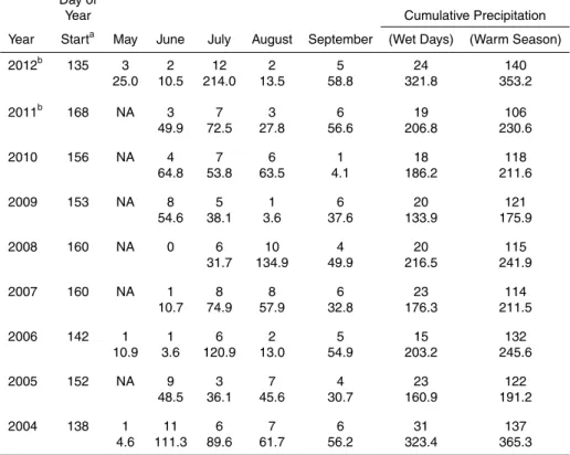
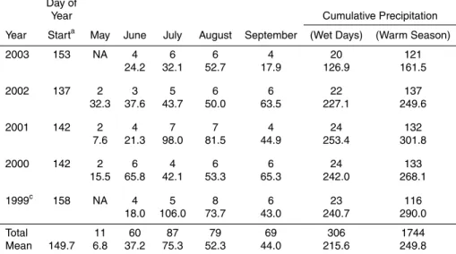
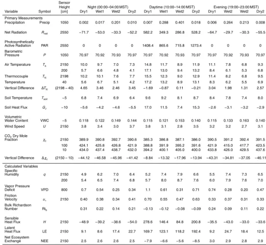
non-normal statistical properties (e.g., Zawadzki, 1973). To study the impact of rain, we followed a methodology similar to that of Turnipseed et al. (2009) and tagged days when the daily rainfall exceeded 3 mm as “wet” days. Table 1 shows the number of wet days for each year and warm-season month within our study. The choice to use

3 mm as the wet-day criteria was a balance between effectively capturing the effect

5

of precipitation and providing enough wet periods to improve the wet-day statistics. Diel patterns for “dry days following a dry day” (designated as Dry1 days), “wet days following a dry day” (designated Wet1 days), “wet days following a wet day” (designated Wet2 days), and “dry days following a wet day” (designated Dry2 days) were analyzed

to determine the effect of a precipitation on the weather and climate as well as the

10

fluxes. If the term “wet days” is used it includes both Wet1 and Wet2 days whereas the term “dry days” includes both Dry1 and Dry2 days. In addition to these categories, we further separated the Dry1 days into sunny (Dry1-Clear) and cloudy (Dry1-Cloudy) days. These techniques are similar to the clustering analysis used by Berkelhammer et al. (2013).

15

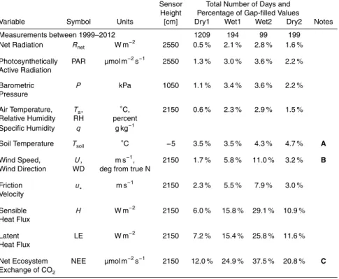
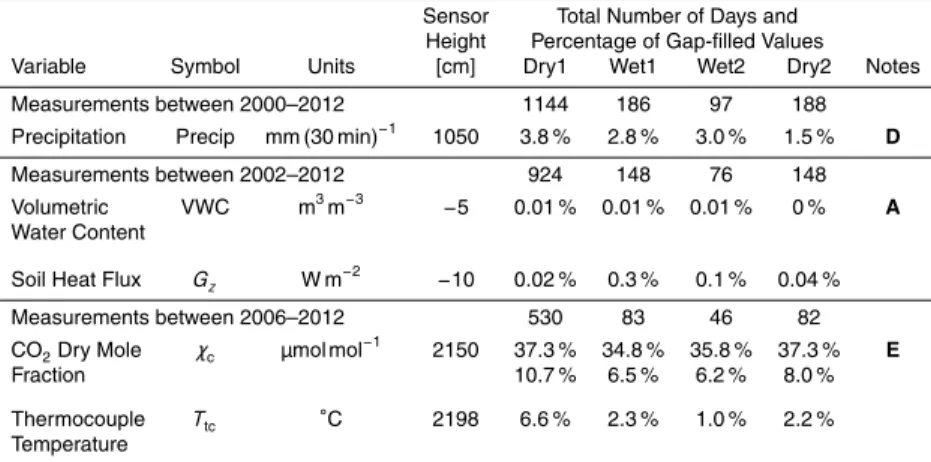
Since not every variable was continuously measured for all 14 years, some variables were necessarily analyzed over shorter periods than others. A summary of the vari-ables studied, the number of days each variable falls into each precipitation category, and gap-filling statistics of selected variables is provided in Table 2. Unless noted oth-erwise, the data analysis used in our study are based on 30 min statistics.

20

In addition to analyzing the mean diel cycle, we also examined the day-to-day vari-ability in the diel cycle by calculating the standard deviation of the 30 min data within each composited time-of-day bin. This statistic will be designated the SD-Bin or vari-ability in our discussion and plots. To further quantify and summarize the main results of our analysis, the diel cycle was broken up into three distinct periods: mid-day (10:00–

25

(11)

BGD

12, 8939–9004, 2015

S. P. Burns et al.

Title Page

Tables Figures

◭ ◮

Back Close

Full Screen / Esc

Discussion

P

a

per

|

Discussion

P

a

per

|

Discussion

P

a

per

|

Discussion

P

a

per

|

around 23:00 MST (see their Fig. 4d). Other flux sites with sloped terrain have shown

distinct differences in the CO2 storage before and after midnight (e.g., Aubinet et al.,

2005) which provides additional motivation for separating the night into two periods. Additional information related to the diel cycle was provided by estimating the top

of the atmosphere incoming solar radiation (Q↓_SW)TOA. The sun position was calculated

5

for the US-NR1 tower latitude and longitude with the SEA-MAT Air-Sea toolbox (Woods Hole Oceanographic Institution, 2013) which uses algorithms based on the 1978

edi-tion of the Almanac for Computers (Nautical Almanac Office, U. S. Naval Observatory).

In order to select the warm-season period, the smoothed seasonal cycle of NEE and the turbulent energy fluxes were calculated using a 20 day mean sliding window

ap-10

plied to the 30 min data. Smoothing removes the effect of large-scale weather patterns

(and precipitation) which typically have a period of 4–7 days. Interannual variability was calculated by taking the standard deviation among the 14 yearly smoothed time se-ries. Since our interest is in the diel cycle, these statistics were determined for mid-day (10:00–14:00 MST), nighttime (00:00–04:00 MST), and the full (24 h) time series.

15

The ecosystem respirationRecowas estimated for each 30 min time period based on

measured nocturnal NEE (both with and without theu∗ filter applied), as well as two

flux-partitioning algorithms that separate NEE intoRecoand gross primary productivity

GPP (Stoy et al., 2006). One algorithm takes into account the seasonal

temperature-dependence ofReco(Reichstein et al., 2005), and the other uses light-response curves

20

(Lasslop et al., 2010). Reichstein and LasslopReco were calculated with on-line

flux-partitioning software (Max Planck Institute for Biogeochemistry, 2013). Further discus-sion of partitioning NEE at the US-NR1 site is provided elsewhere (Zobitz et al., 2008; Bowling et al., 2014).

Near the ground, the bulk Richardson number Ri_bis often used to characterize

stabil-25

ity. Large negative Ribindicates unstable “free convection” conditions and large positive

Rib indicates strong stability (e.g., Kaimal and Finnigan, 1994). In more stable

condi-tions, less mixing is expected and larger vertical scalar gradients should exist (e.g.,

(12)

BGD

12, 8939–9004, 2015

S. P. Burns et al.

Title Page

Tables Figures

◭ ◮

Back Close

Full Screen / Esc

Discussion

P

a

per

|

Discussion

P

a

per

|

Discussion

P

a

per

|

Discussion

P

a

per

|

(z2=21.5 m, around twice canopy height) and lowest (z1=2 m) measurement level

using:

Rib=

g

Ta

(θ2−θ1)(z2−z1)

U2 , (2)

wheregis acceleration due to gravity, Ta is the average air temperature of the layer,

θis potential temperature, andU is the above-canopy horizontal vectorial mean wind

5

speed (i.e.,U =(u2+v2)1/2whereuandv are the streamwise and crosswise planar-fit

horizontal wind components). We did not useU near the ground because this level is

deep within the canopy whereU is small (less than 0.5 m s−1) due to the momentum

absorbed by the needles, branches and boles of the trees. In this respect, the shear-generated turbulence is related to above-canopy wind speed whereas the buoyancy

10

is related to the temperature di_fference between near the ground and the overlying

air. Because Rib is a ratio of two variables, it can become less useful when either the

numerator or denominator becomes very small.

3 Results and discussion

3.1 Typical seasonal cycle and variability

15

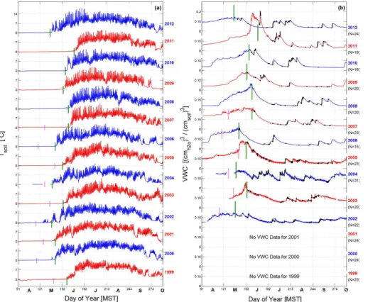
We chose to define the start of the warm-season as the date when diurnal changes in the soil temperature first occurred (i.e., the date of near-complete snowpack abla-tion). For the 14 years of our study, the warm-season start dates ranged from mid-May to mid-June with an average start date of around 1 June (as shown in Fig. 1a and listed in Table 1). Though snow can occur during this period, it is a rare event and

20

(13)

BGD

12, 8939–9004, 2015

S. P. Burns et al.

Title Page

Tables Figures

◭ ◮

Back Close

Full Screen / Esc

Discussion

P

a

per

|

Discussion

P

a

per

|

Discussion

P

a

per

|

Discussion

P

a

per

|

soil moisture content (VWC) reached a maximum (Fig. 1b), and the month following the disappearance of the snowpack was usually when the soil dried out (though there were exceptions, such as 2004). In the warm-season, large precipitation events led to a sharp increase in VWC followed by a gradual return (over several days or weeks) to drier soil conditions. We chose 30 September as the end of the warm-season for

5

reasons described below.

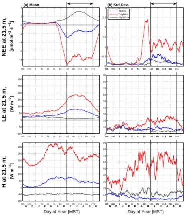
The typical smoothed seasonal cycles of above-canopy NEE, LE andH are shown

in Fig. 2a. For NEE, the dormant period (i.e., when the forest was inactive) was

exem-plified by almost no difference between the daytime and nighttime NEE, which lasted

from roughly early November to mid-April. When daytime NEE switches from positive

10

to negative, it indicates the start of the growing season. The snowmelt period exhibited

strong CO2 uptake because soil respiration was suppressed due to low soil

tempera-ture (Fig. 2a). In February–March, daytimeH reached a maximum because net

radia-tion increased and transpiraradia-tion was small. NighttimeH stayed at around −50 W m−2

throughout the entire year. One might expect nocturnalH in winter to be different than

15

summer, but in winter most of the above-canopyH was due to heat transfer between the

forest canopy and atmosphere, not the atmosphere and snow-covered ground (Burns et al., 2013). Related to LE, there are two interesting observations in Fig. 2a. First, out-side the growing season, daytime LE was larger than nighttime LE. This is presumably because air temperature is higher during the daytime which increases the saturation

20

vapor pressure and results in a larger sublimation/evaporation rate (e.g., Dalton, 1802).

Second, nighttime LE in winter was around 25 W m−2 which decreased to 10 W m−2 in

summer. Despite warmer summer temperatures, we suspect the larger nocturnal LE in winter was due to the ubiquitous presence of a snowpack that serves as a source of sublimation/evaporation for 24 h every day (compared to summer when the ground

25

periodically dries out). Also, winds are much stronger in winter which would promote higher evaporation. In the spring and summer LE increased during the day from around

50 to 150 W m−2due to increased forest transpiration. In July–August, as the soil dried

(14)

BGD

12, 8939–9004, 2015

S. P. Burns et al.

Title Page

Tables Figures

◭ ◮

Back Close

Full Screen / Esc

Discussion

P

a

per

|

Discussion

P

a

per

|

Discussion

P

a

per

|

Discussion

P

a

per

|

and NEE moved closer to having photosynthetic uptake of CO₂ balanced by

respira-tion.

When winds are light and mechanical turbulence is small, decoupling between the air near the ground and above-canopy air can occur (e.g., Baldocchi et al., 2000; Bal-docchi, 2003). The nocturnal NEE data shown in Fig. 2a have been calculated using

5

the friction velocity (u_∗) filtering technique (Goulden et al., 1996) which replaces NEE

during periods of weak ground-atmosphere coupling (u_∗<0.2 m s−1) with an empirical relationship between NEE and soil temperature. This leads to the question of whether

the application of the filtering by u∗ created the apparent increase in nocturnal NEE

(or respiration) during the summer months. In Supplement Fig. S1, we include both

10

the non-u∗filtered NEE along with ecosystem respiration calculated from the algorithm

of Reichstein et al. (2005) and Lasslop et al. (2010). Though the u∗ filter enhanced

the value of ecosystem respiration by around 0.5 µmol m−2s−1compared to unfiltered

NEE, the mid-summer increase was present in both. Ecosystem respiration calculated from the algorithm of Lasslop et al. (2010) was slightly larger than that from Reichstein

15

et al. (2005) which was closer to the measured nocturnal values. Recent research in the ecosystem-flux community has suggested that the standard deviation of the

verti-cal windσw(e.g., Acevedo et al., 2009; Oliveira et al., 2013; Alekseychik et al., 2013;

Thomas et al., 2013) or the Monin–Obukhov stability parameter (e.g., Novick et al.,

2004) are better measures of decoupling thanu_∗; however, the results we show are not

20

going to be strongly a_ffected by which variable is used to determine the coupling state.

The daytime interannual variability of NEE, LE andH was larger than the nighttime

interannual variability (Fig. 2b) due to the wide range of daytime surface solar condi-tions (e.g., clear or cloudy days). The peak in the interannual variability of daytime NEE

during April and May was due to year-to-year differences in the timing of snowmelt and

25

initiation of photosynthetic forest uptake of CO2 at the site (Monson et al., 2005; Hu

et al., 2010a). Though NEE interannual variability peaked at this time, there was no

(15)

BGD

12, 8939–9004, 2015

S. P. Burns et al.

Title Page

Tables Figures

◭ ◮

Back Close

Full Screen / Esc

Discussion

P

a

per

|

Discussion

P

a

per

|

Discussion

P

a

per

|

Discussion

P

a

per

|

The average start of the warm season occurred when daytime NEE uptake was

strong (greater than 8 µmol m−2s−1) and immediately followed the peak in NEE

inter-annual variability (Fig. 2b). There was not a similar increase in NEE variability to mark the end of the warm season; however, the date when daytime NEE decreased sharply was the end of September. For this reason, we chose the end of September as the

5

end of the warm-season. By choosing the end of September we also avoid periods in October when snowfall occurs. On average, the period we chose for the warm season started on 1 June and ended on 30 September as indicated by the vertical lines in Fig. 2.

Based on eight years of precipitation data from a nearby U.S. Climate Reference

Net-10

work (USCRN) site, April had the most precipitation (with a mean of around 120 mm, most all of it falling as snow) followed by July with 90 mm of precipitation (Fig. S2a). April and July were also the months with the largest variability between years and the variations between years were about 50 % of the mean value (Fig. S2b). These trends generally agree with the long-term precipitation measurements from the LTER

15

C-1 (1953–2012) station where the effect of undercatch by the LTER gauge is

notice-able during the winter months. Further discussion on the precipitation measurements used in our study are in Appendix A1.

3.2 The e_ffect of wet conditions on the diel cycle

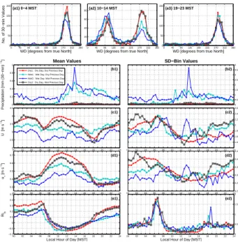
After each day was organized into the precipitation categories described in Sect. 2.3,

20

we observed a peak in precipitation during the early afternoon on wet days as would be expected for a mountain-plain type weather system (Fig. 3b1). Over the 14 years of our study, the average length of time for a dry period was around 2.5 days with a standard deviation of 3 days. Two days in a row with above-average rain (i.e., Wet2 days) was recorded around 90 times out of 1740 total warm-season days between 1999 and 2012

25

(16)

BGD

12, 8939–9004, 2015

S. P. Burns et al.

Title Page

Tables Figures

◭ ◮

Back Close

Full Screen / Esc

Discussion

P

a

per

|

Discussion

P

a

per

|

Discussion

P

a

per

|

Discussion

P

a

per

|

One obvious complication with the precipitation-related analysis is that the open-path

instrumentation (e.g., sonic anemometers) are affected by water droplets, and do not

work properly during heavy precipitation events which is why the percent of gap-filling periods for the fluxes increases on the wet days (Table 2). Though we do not have a way around this issue, we can only point out that the scalar measurements were not

5

affected by precipitation and can provide some degree of insight. When we restricted

the analysis to time periods without any gap-filled flux data, the results are similar to what we are showing here.

Over the next several sections we will examine how the diel cycle of the

measure-ments (winds, soil properties, radiation, scalars, and fluxes) were affected by these

10

di_fferent precipitation states. Because Dry1 conditions were the most common, we will

typically describe the changes or differences relative to the Dry1 state.

3.2.1 Wind, turbulence, and near-ground stability

As mentioned in Sect. 2.1, the above-canopy wind direction at the site is primarily controlled by the large-scale mountain-plain dynamics resulting in directions that were

15

typically either upslope (from the east) or downslope (from the west). At night, the

above-canopy winds were almost exclusively downslope with very little effect from

pre-cipitation except for a small occurrence of upslope flow during Wet2 conditions (i.e., Fig. 3a1). There was a more consistent flow direction in the early morning hours as demonstrated by the higher peak in the frequency distribution of Fig. 3a1 compared to

20

Fig. 3a3. This suggests that the drainage flow became more persistent and consistent as the night progresses. During mid-day, wet conditions had a more frequent occur-rence of upslope winds than downslope winds, whereas during dry days there was nearly an equal number of upslope and downslope winds (Fig. 3a2). This is to be ex-pected because the upslope winds can trigger convection which (potentially) leads to

25

precipitation.

The diel cycle of horizontal wind speed during dry conditions was characterized by

(17)

BGD

12, 8939–9004, 2015

S. P. Burns et al.

Title Page

Tables Figures

◭ ◮

Back Close

Full Screen / Esc

Discussion

P

a

per

|

Discussion

P

a

per

|

Discussion

P

a

per

|

Discussion

P

a

per

|

transition having the lowest wind speed values (Fig. 3c1). On Dry1 and Dry2 days the

wind speed overnight (on average) increased from a minimum of around 2.5 m s−1

at 19:00 MST to a maximum of 4 m s−1 at 04:00 MST. During wet conditions the dip

in wind speed during the transition periods did not exist and the mean wind speed on Wet2 days was typically smaller than other conditions throughout the diel cycle.

5

Mechanical turbulence (characterized by the friction velocityu_∗) generally follows the

pattern of wind speed at night, however, during the daytime, the buoyancy generated by

surface heating enhancedu∗relative to nocturnal values (Fig. 3d1). In Dry1 conditions

the maximum variability inU and u∗ was in the early morning (at around 06:00 MST)

with less variability in the late afternoon and evening.

10

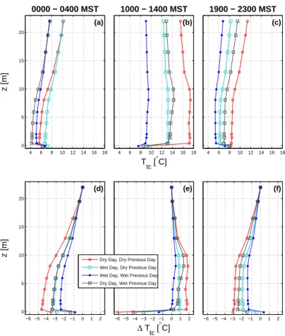
Near-ground vertical air temperature di_fferences are considered because these help

control the near-ground stability (Fig. 4d–f). In Wet2 conditions, the vertical air

temper-ature difference was at a minimum during all times of the day. This is expected during

the daytime because solar radiation, which warms the canopy and ground to create the

air-surface temperature differences, was reduced on Wet2 days (radiation will be

dis-15

cussed in Sect. 3.2.3). In Dry2 conditions during daytime, the mid-canopy was about

1◦C warmer than the air near the ground (Fig. 4e). This stable layer in the lower canopy

did not exist in any other conditions and we presume this state was due to a combina-tion of strong net radiacombina-tion (which warmed the canopy) combined with evaporacombina-tion near the ground (which cooled the ground surface). The soil during a Dry2 day would have

20

recently experienced rain, providing a source of liquid water for evaporation within the

soil. We also note that temperature differences during Dry1 days were the largest of all

precipitation states for the three periods shown in Fig. 4d–f.

To combine the effects of wind speed and temperature differences on atmospheric

stability, the bulk Richardson number Rib is also considered (Fig. 3e1). Following the

25

evening transition, dry conditions tended to result in a more stable atmosphere (Ri_b>

0.2) than that of wet conditions (Rib<0.1). This suggests that there should be larger

(18)

BGD

12, 8939–9004, 2015

S. P. Burns et al.

Title Page

Tables Figures

◭ ◮

Back Close

Full Screen / Esc

Discussion

P

a

per

|

Discussion

P

a

per

|

Discussion

P

a

per

|

Discussion

P

a

per

|

3.2.2 Atmospheric scalars (Ta,q, CO2), soil temperature, soil moisture, and

soil heat flux

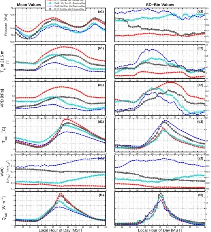
We now consider how air temperature and other scalars change over the diel cycle. Dry1 conditions were associated with slightly higher barometric pressure (Fig. 5a1), rel-atively warmer air temperatures (Fig. 5b1), a drier atmosphere (Fig. 5c1), warmer and

5

drier soils (Fig. 5d1 and e1), and larger soil heat fluxes (Fig. 5f1). Barometric pressure had a mid-morning and evening peak that existed for all precipitation states which are created by thermal tides within the atmosphere (e.g., Lindzen and Chapman, 1969). The variables for Dry1 days generally had smaller variability compared to any of the other conditions (Fig. 5a2–f2) with the one exception being a high variability in VPD

dur-10

ing the Dry1 afternoon and evening period (Fig. 5c2). In contrast to Dry1 days, mean conditions during Wet2 days were associated with (relatively) lower barometric pres-sure and cooler, wetter conditions in the atmosphere and soil.

For Wet2 days, the soil moisture content (VWC) increased by over 50 % and Tsoil

dropped by around 2◦C relative to Dry1 conditions (Table 3 and Fig. 5d1 and e1). The

15

timing of precipitation within the diel cycle is important. For example, on the

morn-ing of Wet1 days, Tsoil was about 1

◦

C larger than in other conditions because on Wet1 days the rain occurred primarily in the afternoon, not the morning (i.e., Fig. 3b1). In fact, 21.5 m air temperature on the morning of Wet1 days was slightly above that of

Dry1 days (Fig. 5b1). The main effect of precipitation on the soil heat flux was between

20

the hours of 11:00 and 18:00 MST, whereGin Dry1 conditions had a peak of 20 W m−2

while in Wet2 conditions the peak was less than 10 W m−2 (Fig. 5f1). At night,G was

similar for all precipitation states suggesting that either the soil was protected from the

effect of changes in nocturnal net radiation by the overlying canopy or else the changes

inRnetwere small enough that the soil temperature was not dramatically affected. This

25

result also implies that increased liquid water in the soil pore space did not significantly

affect the soil thermal conductivity. Though the soil heat flux peaked at around mid-day

(19)

BGD

12, 8939–9004, 2015

S. P. Burns et al.

Title Page

Tables Figures

◭ ◮

Back Close

Full Screen / Esc

Discussion

P

a

per

|

Discussion

P

a

per

|

Discussion

P

a

per

|

Discussion

P

a

per

|

If plots for each precipitation condition are arranged in the order of Dry1, Wet1, Wet2, and Dry2 days the characteristics of a composite summertime cold-front passing the tower can be approximated (Fig. 6). Classical cold-front systems over flat terrain are as-sociated with pre-frontal wind shifts and pressure troughs (e.g., Schultz, 2005). Moun-tains, however, have a large impact on the movement of air masses and can

consider-5

ably alter the classical description of frontal passages (e.g., Egger and Hoinka, 1992; Whiteman, 2000). Our classification of the composite plots as a “frontal passage” is simply because there was colder air present at the site during the Wet1 and Wet2

periods. For example, during Dry1 days the 21.5 m air temperature was around 5◦C

greater than T_soil (Fig. 6b1). As the composite “front” passed by the tower (i.e., Wet1

10

and Wet2 days) 21.5 mTadropped to nearTsoil (Fig. 6b2 and b3) and specific humidity

increased by≈50 % (Fig. 6c2 and c3). After the frontal passage (i.e., Dry2 days), the

21.5 m air temperature returned to being higher than the soil temperature (Fig. 6b4).

During Wet2 days, CO₂dry mole fractionχc within the canopy was elevated relative to

the other conditions (Fig. 6d3). Specific numerical values and a summary of the

atmo-15

spheric conditions for each precipitation state are provided in Table 3.

Taking a closer look at CO₂, we found that above-canopyχcwas largest during Wet2

conditions and lowest in Dry1 conditions with a fairly consistent difference of around 2–

3 µmol mol−1across the entire diel cycle (Fig. 7a). We initially considered this to be an

artifact of dilution due to boundary layer height di_fferences (e.g., Culf et al., 1997),

how-20

ever we ruled this out because the difference was fairly consistent throughout the day

and night when boundary layer heights change dramatically. We confirmed that similar

di_fferences between precipitation states existed using CO₂from a nearby Rocky

Rac-coon site above tree-line on Niwot Ridge (Stephens et al., 2011) (results not shown). Since our analysis uses a composite which approximates a cold-front passage, there is

25

an influence of large-scale weather systems on the overall atmospheric CO₂magnitude

(e.g., Miles et al., 2012; Lee et al., 2012). This suggests that the dependence of

above-canopyχc on the precipitation state was due to either the composition of large-scale

(20)

BGD

12, 8939–9004, 2015

S. P. Burns et al.

Title Page

Tables Figures

◭ ◮

Back Close

Full Screen / Esc

Discussion

P

a

per

|

Discussion

P

a

per

|

Discussion

P

a

per

|

Discussion

P

a

per

|

Within the canopy, this same precipitation-dependent pattern existed in the

morn-ing and durmorn-ing the daytime, however, in the evenmorn-ing,χ_c in dry conditions was about

5–8 µmol mol−1 larger than χc in wet conditions (Fig. 7b–c). These differences clearly

show up in a vertical χc profile (Fig. 8c). To avoid the confounding factor of

synop-tic weather systems, the lower panels in Fig. 8 show the versynop-ticalχ_c differences (∆χ_c)

5

relative to the top tower level (21.5 m a.g.l.). The mid-day ∆χc profile (Fig. 8e) shows

a photosynthetic deficit of around 1 µmol mol−1in the mid-canopy due to vegetative

up-take of CO₂ which is consistent with previous studies at the site (Bowling et al., 2009;

Burns et al., 2011). In the nighttime hours (00:00–04:00 MST) the different precipitation

states did not affect the∆χc profile (Fig. 8d) which contrasts with the late evening∆χc

10

profile that shows a difference of around 5–9 µmol mol−1 between wet and dry

condi-tions within the lower canopy (Fig. 8f).

Synoptic barometric pressure changes have recently been suggested as a

mecha-nism for enhancing the exchange of deep-soil CO₂with the atmosphere, whereas the

upper soil CO2is more influenced by processes such as soil respiration and

pressure-15

pumping (e.g., Sánchez-Cañete et al., 2013). In light of the differences in near-ground

stability during the evening (discussed in Sect. 3.2.1), it seems likely that atmospheric stability was playing a more important role than barometric pressure in controlling the observed nocturnal∆χcdifferences. A close examination of Fig. 8f reveals that the late

evening wet conditions had near-ground to above-canopy ∆χc differences that were

20

around 35 µmol mol−1. In contrast, for all conditions in Fig. 8d and dry conditions in

Fig. 8f the ∆χc differences were greater than 40 µmol mol

−1

(also see Table 3). The

larger ∆χ_c differences in dry conditions are consistent with the near-ground

atmo-spheric stability being larger during dry conditions. We also note that between 00:00–

04:00 MST Rib was generally near or above 0.2 for both wet and dry conditions while

25

in the evening period the wet days had Rib≈0.1. As shown in previous work at the

US-NR1 site (e.g., Schae_ffer et al., 2008a; Burns et al., 2011), _∆χc differences have

a transition region between weakly stable and strongly stable conditions that occurs

(21)

non-BGD

12, 8939–9004, 2015

S. P. Burns et al.

Title Page

Tables Figures

◭ ◮

Back Close

Full Screen / Esc

Discussion

P

a

per

|

Discussion

P

a

per

|

Discussion

P

a

per

|

Discussion

P

a

per

|

turbulent flow. It appears that the stability in the early evening on wet days is such that the atmosphere was slightly unstable which enhanced the vertical mixing and reduced

the vertical∆χc differences. Furthermore, the controls on the stability between Wet1

and Wet2 days were slightly different. On Wet1 evenings, wind speed was slightly

ele-vated (Fig. 3d1) which resulted in less stable conditions. In contrast, on Wet2 evenings

5

it was the reduced vertical temperature differences (Fig. 4f) that was the primary

con-trolling factor in reducing the stability.

3.2.3 Net radiation, turbulent energy fluxes, and net ecosystem exchange of CO2(NEE)

The full diel cycle of net radiation, the turbulent energy fluxes, and NEE are shown

10

in Fig. 9 for mean values (a1–d1) and variability or SD-Bin (a2–d2). In order to bet-ter quantify the impact of precipitation on the fluxes, we have arranged the fluxes by Dry1, Wet1, Wet2, and Dry2 conditions similar to what was shown previously with the scalar measurements (i.e., Fig. 6). This summary, however, only includes mean mid-day (Fig. 10, left-column) and late evening and nighttime values (Fig. 10, right-column).

15

Choosing these specific periods avoids the evening and morning transition periods which are complicated by the fluxes and scalar gradients becoming small and/or chang-ing sign (e.g., Lothon et al., 2014). To make interpretation of the quantitative changes more accessible, each panel in Fig. 10 shows the fractional change from the maximum (or minimum) value within that panel. In addition to the figures, the mean values for

20

each precipitation state are listed in Table 3.

When precipitation occurred, cloudiness increased and net radiation at mid-day

was reduced (Fig. 9a1). Dry1 days had a mean mid-day value of nearly 600 W m−2

which decreased by around 50 % to 300 W m−2 during Wet2 days, then recovered on

Dry2 days to nearly 550 W m−2 (i.e., about 10 % smaller than Rnet during Dry1

con-25

ditions) (Fig. 10a1). The variability of Rnet was similar for all precipitation conditions,

(22)

BGD

12, 8939–9004, 2015

S. P. Burns et al.

Title Page

Tables Figures

◭ ◮

Back Close

Full Screen / Esc

Discussion

P

a

per

|

Discussion

P

a

per

|

Discussion

P

a

per

|

Discussion

P

a

per

|

At night, though the absolute value of the mean net radiation was an order of magni-tude smaller than the daytime values, the fractional changes and pattern of nocturnal

Rnetdue to different precipitation states (Fig. 10a2) were similar to those of mid-dayRnet

(Fig. 10a1). If we assume that wet nights were cloudier than dry nights, the radiative

surface cooling on clear nights was around−70 W m−2while cloudy nights was closer

5

to−30 W m−2. The reduction of the magnitude ofRneton wet nights was primarily due

to changes in cloud cover as well as changes to the turbulent fluxes.

Sensible heat flux during mid-day had a similar pattern to net radiation, with a large

decrease inH (by≈70 %) between Dry1 and Wet2 conditions, followed by an increase

toward Dry1H on Dry2 days (Fig. 10d1). In contrast, latent heat flux followed a slightly

10

di_fferent pattern – the largest mean mid-day LE occurred on a Dry2 day with a value

of around 200 W m−2, which was around 15 % larger than mid-day LE on Dry1 days

(Fig. 10c1). The extra energy used by LE (coupled with slightly lowerRnet values on

Dry2 days) explains why mid-day H only recovered to within 80 W m−2 (or 30 %) of

Dry1H (Fig. 9d1) as dictated by the SEB equation (1).

15

The increased LE values on Dry2 days was presumably due to evaporation of the

intercepted liquid water present on vegetation and in the soil. Because of the e_ffect

of temperature on saturation vapor pressure (and thus VPD) one cannot assume that nocturnal LE is representative of daytime evaporation (e.g., Brutsaert, 1982). To fur-ther explore this issue, we have plotted LE vs. VPD in Fig. 11 where we observe that

20

nocturnal LE in dry conditions was≈10 W m−2with a weak dependence on VPD. This

is consistent with our assumption that there was a small, consistent baseline level of evaporation in dry conditions. Therefore, in Dry1 conditions we can estimate that

evap-oration was ≈10 W m−2 and evapotranspiration was ≈170 W m−2 (based on mid-day

LE, Fig. 10c1). This suggests that, on average, evaporation comprised about 6 % of

25

evapotranspiration in dry conditions. Since net radiation in Dry1 and Dry2 conditions

was similar, we can get a rough estimate of daytime evaporation from the LE diff

er-ence during Dry1 and Dry2 conditions (shown as a black line in Fig. 11a2). As the

(23)

BGD

12, 8939–9004, 2015

S. P. Burns et al.

Title Page

Tables Figures

◭ ◮

Back Close

Full Screen / Esc

Discussion

P

a

per

|

Discussion

P

a

per

|

Discussion

P

a

per

|

Discussion

P

a

per

|

50 W m−2 where it flattens out in drier conditions (for VPD>1.2). Previous research

at the US-NR1 site has shown large differences in transpiration between the

domi-nant tree species (Hu et al., 2010b), but the general relationship between ecosystem-scale transpiration and VPD is similar to what is shown in Fig. 11a2 (Turnipseed et al., 2009). Therefore, following a rain event, daytime evaporation was somewhere between

5

15–50 W m−2(black line in Fig. 11a2) while mid-day evapotranspiration increased from

100–225 W m−2 (Dry2 line in Fig. 11a2). If we take the overall average of this ratio, it

suggests that evaporation comprised about 20 % of evapotranspiration in wet condi-tions.

We also observed that increased LE lasted throughout a Dry2 day until around

10

18:00 MST when LE came within around 10 % of LE in Dry1 conditions (Figs. 9c1 and

11a3). This suggests that the evaporative e_ffect lasted at least 18 h following a

signifi-cant precipitation event. Central to our calculations is the assumption that LE at night was primarily evaporation. Some evidence exists that the needle stomates opening at night combined with cuticular water loss could lead to small amounts of nocturnal

tran-15

spiration (e.g., Novick et al., 2009). If this occurred at US-NR1, it is likely a small effect which is further discussed by Turnipseed et al. (2009). We should also emphasize that our results are mean estimates and the variability around these mean values are large (i.e., as shown in Fig. 11b1–b4). Some of this variability is due to the random nature

of turbulence in the atmosphere, whereas some can be explained by differences in net

20

radiation, atmospheric stability, air temperature, and stomatal control.

The modeling study of Moore et al. (2008) based on sap flow measurements at the US-NR1 site found that transpiration in the warm-season accounted for about 30 % of total evapotranspiration, whereas our findings suggest that transpiration accounted for between 80 % (wet conditions) to 94 % (dry conditions) of evapotranspiration. The

25

(24)

BGD

12, 8939–9004, 2015

S. P. Burns et al.

Title Page

Tables Figures

◭ ◮

Back Close

Full Screen / Esc

Discussion

P

a

per

|

Discussion

P

a

per

|

Discussion

P

a

per

|

Discussion

P

a

per

|

measurement challenges (e.g., Hogg et al., 1997; Wilson et al., 2001; Staudt et al., 2011). The trend toward less evaporation in Dry1 conditions is consistent with a large resistance to evaporation being present when the soil/litter surface under a canopy is dry (Baldocchi and Meyers, 1991). Based on lysimeter measurements of evaporation, it was found that transpiration comprised about 95 % of total evapotranspiration during

5

the growing season in a boreal aspen forest (Blanken et al., 2001). The partitioning of evapotranspiration for a forest is strongly dependent on the vegetation density and

modeling efforts by Lawrence et al. (2007) suggest that, for a canopy density similar to

that of the US-NR1 forest (i.e., LAI≈4), transpiration should be around 80 % of

evap-otranspiration. The spruce forest studied by Staudt et al. (2011) with LAI≈4.8 found

10

that transpiration accounted for about 90 % of total evapotranspiration (in generally dry conditions).

On a larger (global) scale it has recently been suggested from isotope measurements that transpiration contributes 80–90 % to the total annual terrestrial evapotranspiration (Jasechko et al., 2013). This result appears consistent with our estimate of transpiration

15

for the warm-season months; however, similar to the GLEES Rocky Mountain forest site described by Schlaepfer et al. (2014), the US-NR1 forest only has active transpiration for 4–5 months of the year (e.g., Fig. 2a) so the annual contribution of transpiration is much reduced and sublimation of snow plays a significant role.

At night, latent heat flux cooled the surface and was strongly a_ffected by changes

20

in the precipitation state (Fig. 10c2) following a pattern similar to that of nocturnalRnet

(Fig. 10a2). Nocturnal sensible heat flux changed by around 30–40 % during the dif-ferent precipitation states but the pattern did not clearly follow that of eitherRnetor LE

(Fig. 10d2). At night,H generally warms the surface (including the forest vegetation and

other biomass) following the air-surface temperature gradient (i.e., similar to the

verti-25

cal temperature di_fferences shown in Fig. 4d and f). In this way,H acts to compensate

for air-surface temperature differences that might be generated by the surface

cool-ing effects of Rnet and LE. Even though the vertical air temperature differences were

(25)

BGD

12, 8939–9004, 2015

S. P. Burns et al.

Title Page

Tables Figures

◭ ◮

Back Close

Full Screen / Esc

Discussion

P

a

per

|

Discussion

P

a

per

|

Discussion

P

a

per

|

Discussion

P

a

per

|

during Dry2 periods between 00:00–04:00 MST (Fig. 10d2). This is exactly when LE was at a maximum (so evaporative cooling would be expected) and a close look at

Fig. 4f reveals that the temperature difference between the air just above the ground

and soil was larger in Dry2 conditions than Dry1 conditions. We should also note that

what is shown in Fig. 4d and f are vertical air temperature differences which serve as

5

a surrogate for the actual difference between air temperature and the surface elements

(i.e., tree branches, needles, boles, and the soil surface) (e.g., Froelich et al., 2011). As one would expect, daytime NEE was reduced during wet conditions due to

de-creased photosynthetically active radiation (PAR) which is shown as a decrease inRnet

in Fig. 9a1. The ratio between mid-day PAR and R_net was similar for all precipitation

10

states (Table 3) and we will use Rnet as a surrogate for PAR in our discussion. The

Dry2 days were when the forest was most effective at assimilating CO2 and NEE

in-creased by over 3 µmol m−2s−1(≈30 %) between Wet2 and Dry2 days (Fig. 10b1).

Nocturnal NEE was not affected very much (less than 10 %) by changes in the

pre-cipitation state and any effect was overshadowed by the difference between NEE in the

15

late evening compared to the early morning (Figs. 9b1 and 10b2). The models of res-piration by Reichstein and Lasslop produced results similar to the measured nocturnal NEE. The good agreement between the 14 year smoothed nighttime NEE

measure-ment and Reco calculated from the flux-partitioning (i.e., Fig. S1nocturnal ecosystem

respiration signal was, at least for the seasonal-scale, captured at the 21.5 m

measure-20

ment level.

The striking difference between the effect of precipitation on the transport of CO2

(NEE) compared to water vapor (LE) is perplexing because one would expect the

tur-bulence to transport water vapor and CO2in a similar manner. A few possible reasons

for this difference are: (1) soil respiration at the US-NR1 site was not strongly affected

25

by precipitation, (2) long dry periods are rare enough that the Birch effect (i.e., CO₂

(26)

prob-BGD

12, 8939–9004, 2015

S. P. Burns et al.

Title Page

Tables Figures

◭ ◮

Back Close

Full Screen / Esc

Discussion

P

a

per

|

Discussion

P

a

per

|

Discussion

P

a

per

|

Discussion

P

a

per

|

lems related to stable conditions (e.g., Staebler and Fitzjarrald, 2004; Finnigan, 2008;

Aubinet, 2008; Thomas et al., 2013; Alekseychik et al., 2013), or (4) the difference

in vertical location of these two scalar sources (e.g., liquid water evaporates from the

vegetation surfaces as well as at the ground whereas respiration of CO₂occurs almost

exclusively at the ground) caused differences in the sensitivity to precipitation (Edburg

5

et al., 2012). Previous measurements (mostly during the daytime) of soil respiration

R_soil at US-NR1 with a manual chamber system by Scott-Denton et al. (2003, 2006)

found that the dependence of soil respiration on soil moisture over a given summer was small. It has also been suggested by Huxman et al. (2004, 2003) that ecosystem respiration at the US-NR1 site is subject to controls from temperature and radiation

10

as much as from precipitation (in contrast to an arid or semi-arid ecosystem such as

a desert grassland whereReco is strongly dependent on precipitation). The CO2pulse

related to the Birch effect has been detected by eddy-covariance at a wide variety of

ecosystems that are listed in the introduction. For the current study, the relevant results are: (i) the 21.5 m nocturnal NEE measurements were able to detect the increase in

15

nocturnal ecosystem respiration over the warm-season (Fig. 2a), and (ii) the nocturnal

NEE was not strongly a_ffected by precipitation (Fig. 10b2). This suggests that, at the

seasonal/annual time-scale, precipitation plays a minor role in modifying the contribu-tion of ecosystem respiracontribu-tion to the above-canopy NEE for this subalpine ecosystem.

So far we have primarily discussed the mean changes to the ecosystem fluxes due

20

to precipitation. Since these flux calculations are affected by turbulent atmospheric

mo-tions that have a large random component (e.g., Baldocchi, 2003; Vickers et al., 2009) and there is natural day-to-day (and seasonal) variability during a particular time of day, the variability (SD-Bin) around the mean flux value is large (Fig. 9a2–d2). Typi-cally, SD-Bin for the flux is on the order of 50 % of the mean flux. The variability also

25

provides some insight into the various physical processes taking place. For example, Dry1 conditions resulted in the smallest variability for mid-day NEE and LE, but not

for H. Furthermore, in the morning hours (07:00–10:00 MST), the variability of both