www.biogeosciences.net/12/7349/2015/ doi:10.5194/bg-12-7349-2015
© Author(s) 2015. CC Attribution 3.0 License.
The influence of warm-season precipitation on the diel cycle of
the surface energy balance and carbon dioxide at a Colorado
subalpine forest site
S. P. Burns1,2, P. D. Blanken1, A. A. Turnipseed3, J. Hu4, and R. K. Monson5
1Department of Geography, University of Colorado, Boulder, Colorado, USA 2National Center for Atmospheric Research, Boulder, Colorado, USA 32B Technologies, Inc., Boulder, Colorado, USA
4Department of Ecology, Montana State University, Bozeman, Montana, USA
5School of Natural Resources and the Environment, University of Arizona, Tucson, Arizona, USA
Correspondence to:S. P. Burns ([email protected])
Received: 15 May 2015 – Published in Biogeosciences Discuss.: 16 June 2015
Revised: 25 November 2015 – Accepted: 26 November 2015 – Published: 15 December 2015
Abstract. Precipitation changes the physical and biological characteristics of an ecosystem. Using a precipitation-based conditional sampling technique and a 14 year data set from a 25 m micrometeorological tower in a high-elevation sub-alpine forest, we examined how warm-season precipitation affected the above-canopy diel cycle of wind and turbulence, net radiationRnet, ecosystem eddy covariance fluxes
(sensi-ble heatH, latent heat LE, and CO2net ecosystem exchange
NEE) and vertical profiles of scalars (air temperatureTa,
spe-cific humidityq, and CO2dry mole fractionχc). This
anal-ysis allowed us to examine how precipitation modified these variables from hourly (i.e., the diel cycle) to multi-day time-scales (i.e., typical of a weather-system frontal passage).
During mid-day we found the following: (i) even though precipitation caused mean changes on the order of 50–70 % toRnet,H, and LE, the surface energy balance (SEB) was
relatively insensitive to precipitation with mid-day closure values ranging between 90 and 110 %, and (ii) compared to a typical dry day, a day following a rainy day was character-ized by increased ecosystem uptake of CO2(NEE increased
by≈10 %), enhanced evaporative cooling (mid-day LE
in-creased by≈30 W m−2), and a smaller amount of sensible
heat transfer (mid-dayHdecreased by≈70 W m−2). Based
on the mean diel cycle, the evaporative contribution to total evapotranspiration was, on average, around 6 % in dry con-ditions and between 15 and 25 % in partially wet concon-ditions. Furthermore, increased LE lasted at least 18 h following a
rain event. At night, even though precipitation (and accom-panying clouds) reduced the magnitude ofRnet, LE increased
from≈10 to over 20 W m−2 due to increased evaporation.
Any effect of precipitation on the nocturnal SEB closure and NEE was overshadowed by atmospheric phenomena such as horizontal advection and decoupling that create measurement difficulties. Above-canopy mean χc during wet conditions
was found to be about 2–3 µmol mol−1larger thanχ
con dry
days. This difference was fairly constant over the full diel cycle suggesting that it was due to synoptic weather patterns (different air masses and/or effects of barometric pressure). Finally, the effect of clouds on the timing and magnitude of daytime ecosystem fluxes is described.
1 Introduction
Warm-season precipitation is a common perturbation that changes the physical and biological properties of a forest ecosystem. The most obvious effect is the wetting of vege-tation and ground surfaces which provides liquid water for evaporation and changes the surface energy partitioning be-tween sensible heat fluxHand latent heat flux LE (i.e.,
effects on the soil–atmosphere CO2exchange. It can either
displace high CO2-laden air from the soil, or suppress the
release of CO2 because of inhibited diffusion/transport due
to water-filled soil pore space (Hirano et al., 2003; Huxman et al., 2004; Ryan and Law, 2005). The soil and the atmo-sphere near the ground are closely coupled, and therefore soil moisture changes also affect near-ground atmospheric prop-erties (Betts and Ball, 1995; Pattantyús-Ábrahám and Jánosi, 2004).
Rain has been shown to cause short-lived increases in soil respiration by microorganisms (by as much as a factor of ten) in a diverse range of forest and grassland-type ecosys-tems (e.g., Irvine and Law, 2002; Lee et al., 2004; Huxman et al., 2004; Austin et al., 2004; Xu et al., 2004; Tang et al., 2005; Ivans et al., 2006; Misson et al., 2006; Jarvis et al., 2007; Jenerette et al., 2008; Inglima et al., 2009; Savage et al., 2009; Munson et al., 2010; Bowling et al., 2011; Parton et al., 2012). The pulse of CO2emitted from soil that
accom-panies precipitation following a long drought period is one aspect of the so-called Birch effect (named after H. F. Birch (1912–1982), see Jarvis et al. (2007); Unger et al. (2010) for a summary). The timing, size, and duration of the precipi-tation event (as well as the number of previous wet–dry cy-cles) all affect the magnitude of the microbial and plant/tree responses to the water entering the system. The response of soil respiration to a rain pulse typically has an exponential decay with time (Xu et al., 2004; Jenerette et al., 2008). The Birch effect is especially important for the carbon balance in arid or water-limited ecosystems where background soil respiration rates are generally low.
Net ecosystem exchange of CO2(NEE) is calculated from
the above-canopy eddy covariance CO2vertical flux plus the
temporal changes in the CO2dry mole fraction between the
flux measurement-level and the ground (i.e., the CO2
stor-age term). The studies listed in the previous paragraph have used a combination of eddy-covariance, soil chambers, and continuous in situ CO2 mixing ratio measurements to
ex-amine ecosystem responses to precipitation. Many of these studies have also shown that CO2 pulses due to the Birch
effect have an important influence on the seasonal and an-nual budget of NEE for that particular ecosystem (e.g., Lee et al., 2004; Jarvis et al., 2007; Parton et al., 2012). In the current study we will not be concerned with mechanistic or biological aspects of the Birch effect, but instead focus on how precipitation affects above-canopy NEE and any possi-ble implications on the annual carbon budget.
Evaporation from wet surfaces was initially modeled by Penman (1948) using available energy (primarily net ra-diation), the difference between saturation vapor pressure and atmospheric vapor pressure at a given temperature (i.e.,
es−ed, also known as the vapor pressure deficit, VPD), and
aerodynamic resistances to formulate an expression for sur-face LE. The concepts by Penman were extended to include transpiration by Monteith (1965) who introduced the concept of canopy resistance (a resistance to transpiration which is in
series with the aerodynamic resistance, but controlled by the leaf stomates) leading to the Penman–Monteith equation for latent heat flux over dry vegetation. Based on these formula-tions, the fundamental variables which are believed to control evapotranspiration are net radiation, sensible heat flux, atmo-spheric stability (which affects the aerodynamic resistances), stomatal resistance, and VPD. In a fully wet canopy, tran-spiration becomes small and most available energy is used to evaporate liquid water intercepted by the canopy elements and within the soil (e.g., Grelle et al., 1997; Geiger et al., 2003). It has been questioned whether stomates respond to the rate of transpiration rather than VPD (e.g., Monteith, 1995; Pieruschka et al., 2010). It has also been shown that stability/wind speed only has a small direct effect on tran-spiration (e.g., Kim et al., 2014). In our study, we will not consider any effects on transpiration due to seasonal changes in leaf area (e.g., Lindroth, 1985) or variation in soil water potential (e.g., Tan and Black, 1976).
Close to vegetated surfaces, it is known that the atmo-spheric fluxes of CO2and water vapor are correlated to each
other because the leaf stomates control both photosynthesis and transpiration (Monteith, 1965; Brutsaert, 1982; Jarvis and McNaughton, 1986; McNaughton and Jarvis, 1991; Katul et al., 2012; Wang and Dickinson, 2012; Beerling, 2015). There are also temporal changes (and feedbacks) to LE related to boundary layer growth and entrainment which are summarized by van Heerwaarden et al. (2009, 2010). One of the drawbacks to the eddy covariance measurement of LE is that the contributions from the physical process of evap-oration are not easily separated from the biological process of transpiration without making some assumptions of stom-atal behavior (e.g., Scanlon and Kustas, 2010), using isotopic methods (e.g., Yakir and Sternberg, 2000; Williams et al., 2004; Werner et al., 2012; Jasechko et al., 2013; Berkelham-mer et al., 2013), or having additional measurements, such as sap flow (e.g., Hogg et al., 1997; Oishi et al., 2008; Staudt et al., 2011) or weighing lysimeters (e.g., Grimmond et al., 1992; Rana and Katerji, 2000; Blanken et al., 2001). An-other technique uses above-canopy eddy-covariance instru-ments for evapotranspiration coupled with sub-canopy in-struments to estimate evaporation (e.g., Blanken et al., 1997; Law et al., 2000; Wilson et al., 2001; Staudt et al., 2011); this method, however, can have issues with varying flux foot-print sizes (Misson et al., 2007). An accurate way to sep-arate transpiration and evaporation has been a goal of the ecosystem-measurement community for many years, espe-cially an understanding of how this ratio changes during the transition between a wet and dry canopy (e.g., Shuttleworth, 1976, 2007).
pre-cipitation on ecosystem-scale eddy covariance fluxes at the diel (i.e., hourly or “weather-front”) time scale is lacking.
Our study uses 14 years of data from a high-elevation sub-alpine forest AmeriFlux site to explore how warm-season rain events (defined as a daily precipitation total greater than 3 mm) change the mean meteorological variables (horizon-tal wind speedU, air temperatureTa and specific humidity
q), the surface energy fluxes (latent and sensible heat), and
carbon dioxide (both CO2mole fraction and NEE) over the
diel cycle. From this analysis we can evaluate both the mag-nitude and timing of how the energy balance terms and NEE are modified by the presence of rainwater in the soil and on the vegetation. Precipitation is also closely linked to changes in air temperature and humidity as weather fronts and storm systems pass by the site. Since NEE and the energy fluxes depend on meteorological variables such as net radiation, air temperature and VPD, it can be difficult to separate out the effect of precipitation vs. other environmental changes (Turnipseed et al., 2009; Riveros-Iregui et al., 2011).
Though the primary goal of our study is to quantify how precipitation modifies the warm-season mean diel cycle of the measured scalars and fluxes, a secondary goal is to present the 14 year mean and interannual variability of the energy fluxes and NEE measured at the Niwot Ridge Sub-alpine Forest AmeriFlux site. These results will serve as an update to the original set of papers (e.g., Monson et al., 2002; Turnipseed et al., 2002) that examined the ecosystem fluxes from the Niwot Ridge AmeriFlux site over 12 years ago and were based on 2 years of measurements.
2 Data and methods 2.1 Site description
Our study uses data from the Niwot Ridge Subalpine For-est AmeriFlux site (site US-NR1, more information available at http://ameriflux.lbl.gov) located in the Rocky Mountains about 8 km east of the Continental Divide. The US-NR1 mea-surements started in November 1998. The site is on the side of an ancient moraine with granitic-rocky-podzolic soil (typ-ically classified as a loamy sand in dry locations) overlain by a shallow layer (≈10 cm) of organic material (Marr, 1961;
Scott-Denton et al., 2003). The tree density near the US-NR1 27 m walk-up scaffolding tower is around 4000 trees ha−1
with a leaf area index (LAI) of 3.8–4.2 m2m−2 and tree
heights of 12–13 m (Turnipseed et al., 2002; Monson et al., 2010). The subalpine forest surrounding the US-NR1 tower was established in the early 1900s following logging opera-tions, and is primarily composed of subalpine fir (Abies
la-siocarpa var.bifolia) and Englemann spruce (Picea
engel-mannii) west of the tower, and lodgepole pine (Pinus
con-torta) east of the tower. Smaller patches of aspen (Populus
tremuloides) and limber pine (Pinus flexilis) are also present.
Empirical evidence from wind-thrown trees suggest rooting
depths of 40–100 cm which is consistent with depths from similar subalpine forests (e.g., Alexander, 1987) and as dis-cussed in Hu et al. (2010a). Recent analysis of tree ring cores at the site has revealed a significant presence of remnant trees which are older (over 200 years old) and larger than the trees that became established after logging in the early 1900s (R. Alexander, F. Babst, and D. J. P. Moore, University of Ari-zona, unpublished data).
At the US-NR1 subalpine forest, ecosystem processes are closely linked to the presence of snow (Knowles et al., 2014), which typically arrives in October or November, reaches a maximum depth in early April (snow water equivalent (SWE) ≈30 cm), and melts by early June. Sometime in
March or April, the snowpack becomes isothermal (Burns et al., 2013) and liquid water becomes available in the soil, which initiates the photosynthetic uptake of CO2by the
for-est (Monson et al., 2005). The long-term mean annual pre-cipitation at the site is around 800 mm with about 40 % of the total from warm-season rain, which typically occurs ev-ery 2–4 days and has an average daily total of around 4 mm (Hu et al., 2010a). According to the Köppen–Geiger climate classification system (Kottek et al., 2006) the site is type Dfc, which corresponds to a cold, snowy/moist continental cli-mate with precipitation spread fairly evenly throughout the year. The forest could also be classified as climate type H which is sometimes used for mountain locations (Greenland, 2005). The summer precipitation timing is primarily con-trolled by the mountain-plain atmospheric dynamics and thus usually occurs in the afternoon when upslope flows trigger convective thunderstorms (Brazel and Brazel, 1983; Parrish et al., 1990; Whiteman, 2000; Turnipseed et al., 2004; Burns et al., 2011; Zardi and Whiteman, 2013).
2.2 Surface energy balance, measurements, and data details
The terms in the surface energy balance (SEB) are
Ra ≡ Rnet − G − Stot = H + LE +Eadv, (1)
whereRa is the available energy, Rnet is net radiation, G
is soil heat flux at the ground surface, andStot is the heat
and water vapor storage terms in the biomass and airspace between the ground and flux measurement level as well as the energy consumed by photosynthesis. All terms in Eq. (1) have units of W m−2. PositiveR
netindicates radiative
warm-ing of the surface, whereas a positive sign for the other terms in Eq. (1) indicate surface cooling or energy being stored. The Stot terms are typically on the order of 10 % of Rnet
(Turnipseed et al., 2002; Oncley et al., 2007; Lindroth et al., 2010).Stot andG are discussed in detail in Appendix A2.
The horizontal advection of heat and water vapor (Eadv)
im-portant which results in a lack of SEB closure at the US-NR1 site (Turnipseed et al., 2002). In our discussions, the SEB closure fraction refers to the ratio of the sum of the turbulent fluxes to the available energy, i.e., (H+ LE)/Ra.
Rnet was measured at 25 m above ground level (a.g.l.)
with both a net (REBS, model Q-7.1) and four-component (Kipp and Zonen, model CNR1) radiometer. Rnet from the
Q-7.1 sensor is about 15 % closer to closing the SEB than with the CNR1 sensor (Turnipseed et al., 2002; Burns et al., 2012). Since the Q-7.1 radiometer operated during the en-tire 14 year period, it is the primaryRnetsensor in our study.
Calculation of the top-of-the-atmosphere incoming solar ra-diation (Q↓SW)TOA is described in Appendix A1. The
turbu-lent fluxes H and LE were measured at 21.5 m a.g.l.
us-ing standard eddy covariance flux data-processus-ing techniques (e.g., Aubinet et al., 2012) and instrumentation (a 3-D sonic anemometer (Campbell Scientific, model CSAT3), krypton hygrometer (Campbell Scientific, model KH2O), and closed-path infrared gas analyzer; IRGA, LI-COR, model LI-6262). Further details on the specific instrumentation and data-processing techniques are provided elsewhere (Monson et al., 2002; Turnipseed et al., 2002, 2003; Burns et al., 2013). Ad-ditional measurements used in our study are described in Ap-pendix A1 while further details about updates to the US-NR1 flux calculations are in Appendix A3.
2.3 Analysis methods
Precipitation is notoriously difficult to study because of its intermittent, binary nature (e.g., it will often start, stop, re-start, and falls with varying intensity) which leads to non-normal statistical properties (e.g., Zawadzki, 1973). To study the impact of rain, we followed a methodology similar to that of Turnipseed et al. (2009) and tagged days when the daily rainfall exceeded 3 mm as “wet” days. Table 1 shows the number of wet days for each year and warm-season month within our study. The choice to use 3 mm as the wet-day criteria was a balance between effectively capturing the ef-fect of precipitation and providing enough wet periods to improve the wet-day statistics. If we designate the precip-itation state of the preceding day with a lower-case let-ter, then diel patterns for “dry days following a dry day” (dDry days), “wet days following a dry day” (dWet days), “wet days following a wet day” (wWet days), and “dry days following a wet day” (wDry days) were analyzed to deter-mine the effect of precipitation on the weather and climate as well as the fluxes. The term “wet days” includes both dWet and wWet days whereas the term “dry days” includes both dDry and wDry days. In addition to these categories, we further separated the dDry days into sunny (dDry-Clear) and cloudy (dDry-Cloudy) days. These techniques are similar to the clustering analysis used by Berkelhammer et al. (2013).
Since not every variable was continuously measured for all 14 years, some variables were necessarily analyzed over shorter periods than others. A summary of the variables
stud-ied, the number of days each variable falls into each precipi-tation category, and gap-filling statistics of selected variables is provided in Table 2. Unless noted otherwise, the data anal-ysis used in our study are based on 30 min statistics.
In addition to analyzing the mean diel cycle, we also ex-amined the day-to-day variability in the diel cycle by calcu-lating the standard deviation of the 30 min data within each composited time-of-day bin. This statistic will be designated the SD-Bin or variability. For brevity, the focus in the cur-rent paper is on the mean results; more details on variability can be found within the discussion paper (i.e., Burns et al., 2015). To further quantify and summarize the main results of our analysis, the diel cycle was broken up into three distinct periods: mid-day (10:00–14:00 MST), late evening (19:00– 23:00 MST), and nighttime (00:00–04:00 MST). Motivation for breaking up the night into two distinct periods is provided by Burns et al. (2011) who showed that the variability of the turbulence activity (expressed by the SD-Bin of the standard deviation of the vertical wind) increased by about a factor of two at around 23:00 MST (see their Fig. 4d). Other flux sites with sloped terrain have also shown distinct differences in the CO2 storage before and after midnight (e.g., Aubinet et al.,
2005). Choosing these particular periods avoids the evening and morning transition periods which are complicated by the fluxes and scalar gradients becoming small and/or changing sign (e.g., Lothon et al., 2014).
In order to select the warm-season period, the smoothed seasonal cycle of NEE and the turbulent energy fluxes were calculated using a 20-day mean sliding window ap-plied to the 30 min data. Smoothing removes the effect of large-scale weather patterns (and precipitation) which typi-cally have a period of 4–7 days. Interannual variability was calculated by taking the standard deviation among the 14 yearly smoothed time series. Since our interest is in the diel cycle, these statistics were determined for mid-day (10:00–14:00 MST), nighttime (00:00–04:00 MST), and the full (24 h) time series.
The ecosystem respiration Reco was estimated for each
30 min time period based on measured nocturnal NEE (both with and without the friction velocity (u∗) filter applied),
as well as two flux-partitioning algorithms that separate NEE into Reco and gross primary productivity GPP (Stoy
et al., 2006). One algorithm takes into account the seasonal temperature-dependence of Reco (Reichstein et al., 2005),
and the other uses light-response curves (Lasslop et al., 2010). Reichstein and LasslopRecowere calculated with
on-line flux-partitioning software (Max Planck Institute, 2013). With regard to our analysis,Recofrom the flux-partitioning
methods and measured nocturnal NEE produced very simi-lar results which are shown in Burns et al. (2015). Therefore, we only use the measured nocturnal NEE herein, and will not include the Reichstein or LasslopRecoresults. Unless noted
otherwise, we will use theu∗ filtered NEE in our analysis.
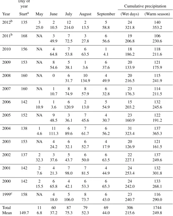
Table 1.Precipitation statistics for the US-NR1 AmeriFlux site. The number of days with a daily precipitation greater than 3 mm day−1for
each year and month is shown. These are defined as “wet” days in the analysis (see text for details). If the warm season started in June, then the May column is filled with “NA”. The total cumulative precipitation from the wet days is given immediately below the number of days. In the two right-hand columns the cumulative precipitation from the wet days only and from all days within the warm season are provided. Precipitation units are mm.
Day of
year Cumulative precipitation
Year Starta May June July August September (Wet days) (Warm season)
2012b 135 3 2 12 2 5 24 140
25.0 10.5 214.0 13.5 58.8 321.8 353.2
2011b 168 NA 3 7 3 6 19 106
49.9 72.5 27.8 56.6 206.8 230.6
2010 156 NA 4 7 6 1 18 118
64.8 53.8 63.5 4.1 186.2 211.6
2009 153 NA 8 5 1 6 20 121
54.6 38.1 3.6 37.6 133.9 175.9
2008 160 NA 0 6 10 4 20 115
31.7 134.9 49.9 216.5 241.9
2007 160 NA 1 8 8 6 23 114
10.7 74.9 57.9 32.8 176.3 211.5
2006 142 1 1 6 2 5 15 132
10.9 3.6 120.9 13.0 54.9 203.2 245.6
2005 152 NA 9 3 7 4 23 122
48.5 36.1 45.6 30.7 160.9 191.2
2004 138 1 11 6 7 6 31 137
4.6 111.3 89.6 61.7 56.2 323.4 365.3
2003 153 NA 4 6 6 4 20 121
24.2 32.1 52.7 17.9 126.9 161.5
2002 137 2 3 5 6 6 22 137
32.3 37.6 43.7 50.0 63.5 227.1 249.6
2001 142 2 4 7 7 4 24 132
7.6 21.3 98.0 81.5 44.9 253.4 301.8
2000 142 2 6 4 6 6 24 133
15.5 65.8 42.1 53.3 65.3 242.0 268.1
1999c 158 NA 4 5 8 6 23 116
18.0 106.0 73.7 43.0 240.7 290.0
Total 11 60 87 79 69 306 1744
Mean 149.7 6.8 37.2 75.3 52.3 44.0 215.6 249.8
aThis column indicates the day of year the warm season started based on diel changes in the soil temperature as shown in Fig. 1. bFor 2011 and 2012, precipitation from the NOAA US Climate Reference Network (USCRN; Diamond et al., 2013) MRS “Hills
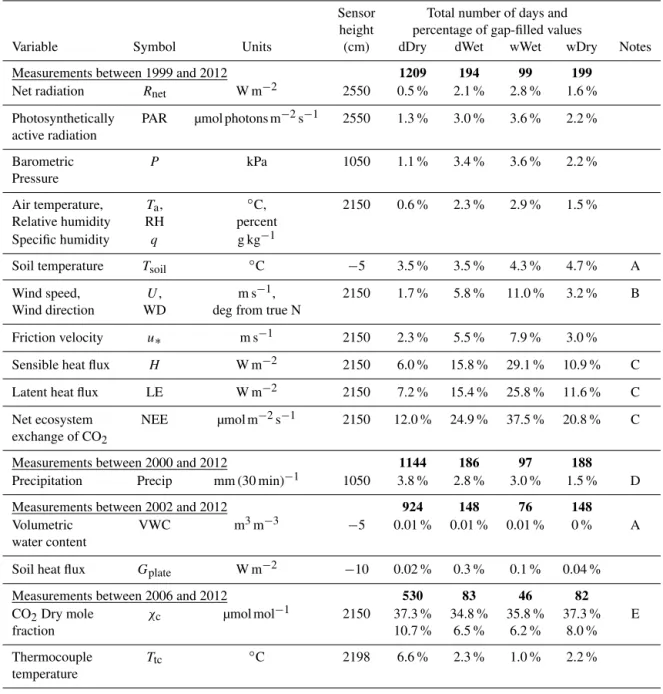
Table 2.Variables, symbols, units, and height above ground of measurements along with the number of days each variable falls within
each precipitation category. Where appropriate, the percentage gap-filled 30 min data for each particular variable is shown. If any variable is missing for a 30 min period, then all variables within that particular group are excluded.
Sensor Total number of days and
height percentage of gap-filled values
Variable Symbol Units (cm) dDry dWet wWet wDry Notes
Measurements between 1999 and 2012 1209 194 99 199
Net radiation Rnet W m−2 2550 0.5 % 2.1 % 2.8 % 1.6 %
Photosynthetically PAR µmol photons m−2s−1 2550 1.3 % 3.0 % 3.6 % 2.2 %
active radiation
Barometric P kPa 1050 1.1 % 3.4 % 3.6 % 2.2 %
Pressure
Air temperature, Ta, ◦C, 2150 0.6 % 2.3 % 2.9 % 1.5 %
Relative humidity RH percent
Specific humidity q g kg−1
Soil temperature Tsoil ◦C −5 3.5 % 3.5 % 4.3 % 4.7 % A
Wind speed, U, m s−1, 2150 1.7 % 5.8 % 11.0 % 3.2 % B
Wind direction WD deg from true N
Friction velocity u∗ m s−1 2150 2.3 % 5.5 % 7.9 % 3.0 %
Sensible heat flux H W m−2 2150 6.0 % 15.8 % 29.1 % 10.9 % C
Latent heat flux LE W m−2 2150 7.2 % 15.4 % 25.8 % 11.6 % C
Net ecosystem NEE µmol m−2s−1 2150 12.0 % 24.9 % 37.5 % 20.8 % C
exchange of CO2
Measurements between 2000 and 2012 1144 186 97 188
Precipitation Precip mm (30 min)−1 1050 3.8 % 2.8 % 3.0 % 1.5 % D
Measurements between 2002 and 2012 924 148 76 148
Volumetric VWC m3m−3 −5 0.01 % 0.01 % 0.01 % 0 % A
water content
Soil heat flux Gplate W m−2 −10 0.02 % 0.3 % 0.1 % 0.04 %
Measurements between 2006 and 2012 530 83 46 82
CO2Dry mole χc µmol mol−1 2150 37.3 % 34.8 % 35.8 % 37.3 % E
fraction 10.7 % 6.5 % 6.2 % 8.0 %
Thermocouple Ttc ◦C 2198 6.6 % 2.3 % 1.0 % 2.2 %
temperature
is provided elsewhere (Zobitz et al., 2008; Bowling et al., 2014).
Near the ground, the bulk Richardson number Ribis often
used to characterize stability. Large negative Rib indicates
unstable “free convection” conditions and large positive Rib
indicates strong stability. In more stable conditions, less mix-ing is expected and larger vertical scalar gradients should exist. We calculated Rib between the highest (z2=21.5 m,
around twice canopy height) and lowest (z1=2 m)
measure-ment level using Rib= g
Ta
(θ2−θ1)(z2−z1)
U2 , (2)
wheregis acceleration due to gravity,Tais the average air
temperature of the layer,θ is potential temperature, andU
is the above-canopy horizontal vectorial mean wind speed (i.e.,U= (u2+v2)1/2whereuandvare the streamwise and
crosswise planar-fit horizontal wind components). We did not useUnear the ground because this level is deep within
the canopy whereUis small (less than 0.5 m s−1) due to the
momentum absorbed by the needles, branches and boles of the trees. In this respect, the shear-generated turbulence is related to above-canopy wind speed whereas the buoyancy is related to the above-canopy/near-ground temperature differ-ence.
3 Results and discussion
3.1 Typical seasonal cycle and variability
We chose to define the start of the warm season as the date when diurnal changes in the soil temperature first oc-curred (i.e., the date of near-complete snowpack ablation). For the 14 years of our study, the warm-season start dates ranged from mid-May to mid-June with an average start date of around 1 June (as shown in Fig. 1a and listed in Ta-ble 1). Though snow can occur during the warm season, it is a rare event and usually melts quickly. The start of the growing-season (based on NEE, as described in Hu et al., 2010a) typically preceded the start of the warm season by 2–4 weeks (Fig. 1a). The warm-season start date was also around the time that the volumetric soil moisture content (VWC) reached a maximum (Fig. 1b), and the month follow-ing the disappearance of the snowpack was usually when the soil dried out (though there were exceptions, such as 2004). In the warm season, large precipitation events led to a sharp increase in VWC followed by a gradual return (over several days or weeks) to drier soil conditions. We chose 30 Septem-ber as the end of the warm season for reasons described be-low.
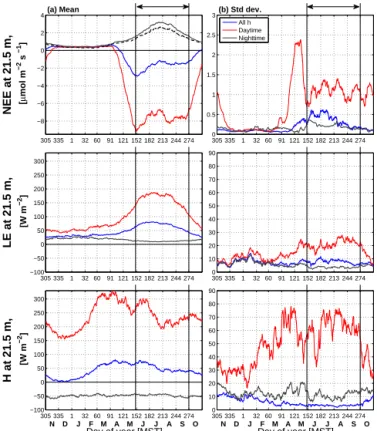
The typical smoothed seasonal cycles of above-canopy NEE, LE and H are shown in Fig. 2a. For NEE, the
dor-mant period (i.e., when the forest was inactive) was exem-plified by almost no difference between the daytime and
nighttime NEE, which lasted from roughly early Novem-ber to mid-April. When daytime NEE switches from pos-itive to negative, it indicates the start of the growing sea-son. The snowmelt period exhibited strong CO2uptake
be-cause soil respiration was suppressed due to low soil tem-perature (Fig. 2a). In February–March, daytimeH reached
a maximum because net radiation increased and transpira-tion was small. NighttimeH stayed at around−50 W m−2
throughout the entire year. One might expect nocturnal H
in winter to be different than summer, but in winter most of the above-canopy H was due to heat transfer between
the forest canopy and atmosphere, not the atmosphere and snow-covered ground (Burns et al., 2013). Related to LE, there are two interesting observations in Fig. 2a. First, out-side the growing season, daytime LE was larger than night-time LE. This is presumably because air temperature is higher during the daytime which increases the saturation va-por pressure and results in a larger sublimation/evava-poration rate (e.g., Dalton, 1802). Second, nighttime LE in winter was around 25 W m−2which decreased to 10 W m−2in
sum-mer. Despite warmer summer temperatures, we suspect the larger nocturnal LE in winter was due to the ubiquitous presence of a snowpack that serves as a source of subli-mation/evaporation for 24 h every day (compared to sum-mer when the ground periodically dries out). Also, winds are much stronger between November and February which promotes higher sublimation/evaporation. In the spring and summer LE increased during the day from around 50 to 150 W m−2primarily due to increased forest transpiration as
well as increased VPD. In July–August, as the soil dried out and warmed up, soil microbial activity increased (e.g., Scott-Denton et al., 2006), and NEE moved closer to having pho-tosynthetic uptake of CO2balanced by respiration.
When winds are light and mechanical turbulence is small, decoupling between the air near the ground and above-canopy air can occur (e.g., Baldocchi et al., 2000; Baldocchi, 2003). The nocturnal NEE data shown in Fig. 2a have been calculated both with (solid line) and without (dashed line) the
u∗filtering technique (Goulden et al., 1996) which replaces
NEE during periods of weak ground-atmosphere coupling (u∗ < 0.2 m s−1) with an empirical relationship between
NEE and soil temperature. Though the u∗ filter enhanced
the value of nocturnal NEE by around 0.5 µmol m−2s−1
compared to unfiltered NEE, the mid-summer increase was present in both. Recent research in the ecosystem-flux com-munity has suggested that the standard deviation of the verti-cal windσw(e.g., Acevedo et al., 2009; Oliveira et al., 2013;
Alekseychik et al., 2013; Thomas et al., 2013) or the Monin– Obukhov stability parameter (e.g., Novick et al., 2004) are better measures of decoupling thanu∗; however, the results
we show are not going to be strongly affected by which vari-able is used to determine the coupling state.
The daytime interannual variability of NEE, LE and H
91 121 152 182 213 244 274 0
0.15 0 0.15 0 0.15 0 0.15 0 0.15 0 0.15 0 0.15 0 0.15 0 0.15 0 0.15 0 0.15 0 0.15 0 0.15 0 0.15 0.3
1999
No VWC Data for 1999
(N=23)
2000
No VWC Data for 2000
(N=24)
2001
No VWC Data for 2001
(N=24)
2002
(N=22)
2003
(N=20)
2004
(N=31)
2005
(N=23)
2006
(N=15)
2007
(N=23)
2008
(N=20)
2009
(N=20)
2010
(N=18)
2011
(N=19)
2012
(N=24)
Day of Year [MST]
A M J J A S O
(b)
VWC [(cm
h2o
)
3 / (cm
soil
)
3 ]
91 121 152 182 213 244 274
0 7 0 7 0 7 0 7 0 7 0 7 0 7 0 7 0 7 0 7 0 7 0 7 0 7 0 7 14
1999
2000
2001
2002
2003
2004
2005
2006
2007
2008
2009
2010
2011
2012
Day of Year [MST]
A M J J A S O
(a)
T soil
[
° C]
Figure 1. (a)Soil temperature and(b)soil moisture for years 1999 to 2012. In(b), the black dots indicate wet days and the number of wet
days for each year is shown to the right of the panel underneath the year. The warm-season start date was chosen based on the date that the soil temperature diurnal changes started to occur as indicated by the vertical green lines. The vertical mauve lines for years 1999–2007 are the start date of the growing season as determined by Hu et al. (2010a). Starting with year 2006, a single set of soil sensors at a depth of 5 cm were used (see Appendix A1 for details).
(e.g., clear or cloudy days). The peak in the interannual vari-ability of daytime NEE during April and May was due to year-to-year differences in the timing of snowmelt and initia-tion of photosynthetic forest uptake of CO2at the site
(Mon-son et al., 2005; Hu et al., 2010a). Though NEE interannual variability peaked at this time, there was no corresponding peak in LE orHvariability.
The average start of the warm season occurred when day-time NEE uptake was strong (greater than 8 µmol m−2s−1)
and immediately followed the peak in NEE interannual vari-ability (Fig. 2b). There was not a similar increase in NEE variability to mark the end of the warm season; however, the date when daytime NEE decreased sharply was the end of September. For this reason, we chose the end of Septem-ber as the end of the warm season. By choosing the end of
September we also avoid periods in October when snowfall occurred.
morn-0 0.5 1 1.5 2 2.5
3(b) Std dev.
305 335 1 32 60 91 121 152 182 213 244 274
All h Daytime Nighttime
−8 −6 −4 −2 0 2 4
NEE at 21.5 m, [
µ
mol m
−2
s
−1
]
(a) Mean
305 3351 32 60 91 121 152 182 213 244 274
−100 −50 0 50 100 150 200 250 300
LE at 21.5 m,
[W m
−2
]
305 3351 32 60 91 121 152 182 213 244 274 0
10 20 30 40 50 60 70 80 90
305 335 1 32 60 91 121 152 182 213 244 274
−100 −50 0 50 100 150 200 250 300
H at 21.5 m,
[W m
−2
]
305 3351 32 60 91 121 152 182 213 244 274
N D J F M A M J J A S O Day of year [MST]
0 10 20 30 40 50 60 70 80 90
305 335 1 32 60 91 121 152 182 213 244 274
N D J F M A M J J A S O Day of year [MST]
Figure 2.Fourteen-year(a)mean and(b)interannual standard
de-viation (n=14 years) of (top) CO2net ecosystem exchange NEE, (middle) latent heat flux LE, and (bottom) sensible heat fluxH. To remove the effects of short-term changes due to weather each 30 min yearly time series is averaged with a 20-day mean sliding window. In all panels, the statistics are calculated for all hours, day-time (10:00–14:00 MST), and nightday-time (00:00–04:00 MST) peri-ods following the legend in(b). In(a), nocturnal NEE calculated
without theu∗ filter is shown as a dashed line. These data were
collected between 1 November 1998 and 31 October 2012. Vertical lines with the arrows indicate the average warm-season period used for our study.
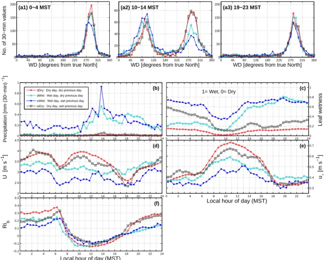
ing precipitation occurred on wWet days (i.e., Fig. 3b). The leaf wetness data reveal that, on average, dDry days had mean value less than 0.2, while wet periods were closer to 0.8 (Fig. 3c). On wDry days there was a steady decrease in leaf wetness from midnight until the early morning hours. All precipitation states had a minimum in leaf wetness be-tween around 08:00–10:00 MST which is likely related to a large-scale phenomena, such as the entrainment of dry air at the top of the boundary layer.
One obvious complication with the precipitation-related analysis is that the open-path instrumentation (e.g., sonic anemometers) are affected by water droplets, and do not work properly during heavy precipitation events which is why the percent of gap-filling periods for the fluxes increases on the wet days (Table 2). Though we do not have a way around this issue, we can only point out that the scalar mea-surements were not affected by precipitation, which provides
some degree of insight. When we restricted the analysis to time periods without any gap-filled flux data, the results are similar to what we show here (see Appendix A5 for an exam-ple).
Over the next several sections we will examine how the diel cycle of the measurements (winds, soil properties, ra-diation, scalars, and fluxes) were affected by these different precipitation states. Because dDry conditions were the most common, we will typically describe the changes or differ-ences relative to the dDry state.
3.2.1 Wind, turbulence, vertical temperature profiles, and near-ground stability
As mentioned in Sect. 2.1, the above-canopy wind direction at the site is primarily controlled by the large-scale mountain-plain dynamics resulting in directions that were typically ei-ther upslope (from the east) or downslope (from the west). At night, the above-canopy winds were almost exclusively downslope with very little effect from precipitation except for a small occurrence of upslope flow during wWet condi-tions (i.e., Fig. 3a1). There was a more consistent flow direc-tion in the early morning hours as demonstrated by the higher peak in the frequency distribution of Fig. 3a1 compared to Fig. 3a3. This suggests that the drainage flow became more persistent and consistent as the night progresses. During mid-day, wet conditions had a more frequent occurrence of ups-lope winds than downsups-lope winds, whereas during dry days there was nearly an equal number of upslope and downslope winds (Fig. 3a2). This is to be expected because the upslope winds can trigger convection which (potentially) leads to pre-cipitation.
The diel cycle of horizontal wind speed during dry condi-tions was characterized by a dip of about 1 m s−1during the
morning and evening transitions, with the evening transition having the lowest wind speed values (Fig. 3d). On dDry and wDry days the wind speed overnight (on average) increased from a minimum of around 2.5 m s−1at 19:00 MST to a
max-imum of 4 m s−1 at 04:00 MST. During wet conditions the
dip in wind speed during the transition periods did not exist and the mean wind speed on wWet days was typically smaller than other conditions throughout the diel cycle. Mechanical turbulence (characterized by the friction velocityu∗)
gener-ally follows the pattern of wind speed at night; however, dur-ing the daytime, the buoyancy generated by surface heatdur-ing enhancedu∗ relative to nocturnal values (Fig. 3e). In dDry
conditions the maximum variability inU andu∗was in the
early morning (at around 06:00 MST) with less variability in the late afternoon and evening.
tem-0 45 90 135 180 225 270 315 360 0
50 100 150 200
(a1) 0−4 MST
WD [degrees from true North]
0 45 90 135 180 225 270 315 360
0 20 40 60 80
WD [degrees from true North]
(a2) 10−14 MST
0 45 90 135 180 225 270 315 360
0 50 100 150 200
(a3) 19−23 MST
WD [degrees from true North]
0 2 4 6 8 10 12 14 16 18 20 22 24
0 0.2 0.4 0.6 0.8 1
Precipitation [mm (30−min)
−1
]
(b)
0 2 4 6 8 10 12 14 16 18 20 22 240
0.2 0.4 0.6 0.8 1
Leaf wetness
1= Wet, 0= Dry (c)
0 2 4 6 8 10 12 14 16 18 20 22 24
2 2.5 3 3.5 4 4.5
U [m s
−1
]
(d) dDry: Dry day, dry previous day
dWet: Wet day, dry previous day wWet: Wet day, wet previous day wDry: Dry day, wet previous day
0 2 4 6 8 10 12 14 16 18 20 22 24
0.3 0.4 0.5 0.6 0.7
u∗
[m s
−1
]
(e)
Local hour of day (MST)
0 2 4 6 8 10 12 14 16 18 20 22 24
−0.2 −0.1 0 0.1 0.2 0.3 0.4 0.5
Rib
(f)
Local hour of day (MST)
No. of 30−min values
Figure 3.Frequency distributions of wind direction WD for different precipitation states for(a1)nighttime (00:00–04:00 MST)(a2)mid-day
(10:00–14:00 MST), and(a3)late evening (19:00–23:00 MST) periods. Because there are a different number of 30 min periods within each
precipitation state, the frequency distributions were created by randomly selecting 800 values for each precipitation state. Below(a1–a3), the
mean warm-season diel cycle of(b)precipitation,(c)leaf wetness,(d)21.5 m horizontal wind speedU,(e)21.5 m friction velocityu∗, and
(f)bulk Richardson number Ribare shown. These composites are from 30 min data during the warm season between years 1999 and 2012.
For all panels, each line represents a different precipitation state as shown in the legend of panel(b).
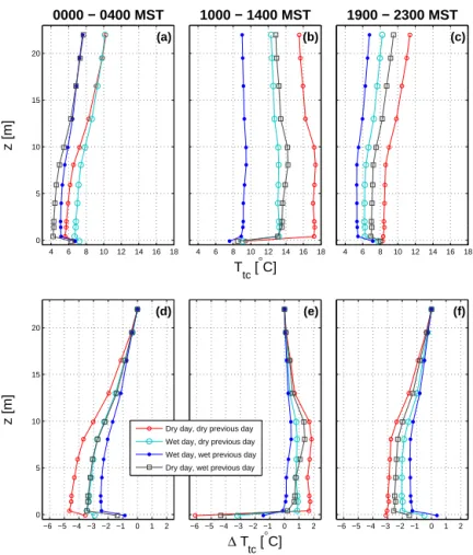
perature differences, was reduced on wWet days (radiation will be discussed in Sect. 3.2.4). In wDry conditions dur-ing daytime, the mid-canopy was about 1◦C warmer than
the air near the ground (Fig. 4e). This stable layer in the lower canopy did not exist in any other conditions and we presume this state was due to a combination of strong net ra-diation (which warmed the canopy) combined with evapora-tion near the ground (which cooled the ground surface). The soil during a wDry day would have recently experienced rain, providing a source of liquid water for evaporation within the soil. We also note that temperature differences during dDry days were the largest of all precipitation states for the three periods shown in Fig. 4d–f.
To combine the effects of wind speed and temperature dif-ferences on atmospheric stability, the bulk Richardson num-ber Rib is also considered (Fig. 3f). Following the evening
transition, dry conditions tended to result in a more stable
atmosphere (Rib>0.2) than that of wet conditions (Rib<
0.1). This suggests that there should be larger vertical scalar
differences (i.e., less vertical mixing) during the late evening period of dry days.
3.2.2 Atmospheric scalars (Ta,q), soil temperature, soil
moisture, and soil heat flux
com-4 6 8 10 12 14 16 18 0
5 10 15 20
z [m]
(a)
0000 − 0400 MST
−6 −5 −4 −3 −2 −1 0 1 2
0 5 10 15 20
(d)
z [m]
4 6 8 10 12 14 16 18
(b)
T tc [
°C]
1000 − 1400 MST
−6 −5 −4 −3 −2 −1 0 1 2
(e)
∆ T tc [
°C]
4 6 8 10 12 14 16 18
(c)
1900 − 2300 MST
−6 −5 −4 −3 −2 −1 0 1 2
(f)
Dry day, dry previous day Wet day, dry previous day Wet day, wet previous day Dry day, wet previous day
Figure 4.Vertical profiles of mean warm-season thermocouple air temperatureTtcand soil temperatureTsoil(at a depth of 5 cm) for (left) nighttime (00:00–04:00 MST), (middle) mid-day (10:00–14:00 MST), and (right) late evening (19:00–23:00 MST). The upper row is the absolute temperature, while the bottom row is the temperature difference relative to the highest level (21.98 m). Each line represents a different precipitation state as shown in the legend. These measurements are from the warm season in years 2006–2012.
pared to any of the other conditions with the one excep-tion being a high variability in VPD during the dDry after-noon and evening period (Burns et al., 2015). In contrast to dDry days, mean conditions during wWet days were associ-ated with (relatively) lower barometric pressure and cooler, wetter conditions in the atmosphere and soil.
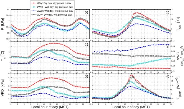
For wWet days, the soil moisture content (VWC) increased by over 50 % and Tsoil dropped by around 2◦C relative to
dDry conditions (Table 3 and Fig. 5b and d). The timing of precipitation within the diel cycle is important. For example, on the morning of dWet days,Tsoilwas about 1◦C larger than
in other conditions because on dWet days the rain occurred primarily in the afternoon, not the morning (i.e., Fig. 3b). In fact, 21.5 m air temperature on the morning of dWet days was nearly the same as that of dDry days (Fig. 5c). The main ef-fect of precipitation on the deep-soil heat flux was between the hours of 11:00 and 18:00 MST, whereGplatein dDry
con-ditions had a peak of 20 W m−2while in wWet conditions the
peak was less than 10 W m−2(Fig. 5f). At night,Gplatewas
similar for all precipitation states suggesting that either the
deeper (10 cm) soil was protected from the effect of changes in nocturnal net radiation by the overlying canopy and soil or else the changes inRnetwere small enough that the deep soil
temperature was not dramatically affected. Though the soil heat flux peaked at around mid-day, the 5 cm soil tempera-ture peaked two hours later at around 14:00 MST.
If plots for each precipitation condition are arranged in the order of dDry, dWet, wWet, and wDry days, the characteris-tics of a composite summertime cold-front passing the tower can be approximated (Fig. 6). Classical cold-front systems over flat terrain are associated with pre-frontal wind shifts and pressure troughs (e.g., Schultz, 2005). Mountains, how-ever, have a large impact on the movement of air masses and can considerably alter the classical description of frontal pas-sages (e.g., Egger and Hoinka, 1992; Whiteman, 2000). Our classification of the composite plots as a “frontal passage” is simply because there was colder air present at the site during the dWet and wWet periods. For example, during dDry days the 21.5 m air temperature was around 5◦C greater thanT
soil
0 2 4 6 8 10 12 14 16 18 20 22 24 70.85 70.9 70.95 71 71.05 71.1
P [kPa]
(a)
dDry: Dry day, dry previous day dWet: Wet day, dry previous day
wWet: Wet day, wet previous day wDry: Dry day, wet previous day
0 2 4 6 8 10 12 14 16 18 20 22 24
6 8 10 12 14 16 T a [ ° C] (c)
0 2 4 6 8 10 12 14 16 18 20 22 24
0 0.2 0.4 0.6 0.8 1 1.2 1.4
VPD [kPa]
(e)
Local hour of day (MST)
0 2 4 6 8 10 12 14 16 18 20 22 246
7 8 9 10 11 12 T soil [ ° C] (b)
0 2 4 6 8 10 12 14 16 18 20 22 240.11
0.12 0.13 0.14 0.15 0.16 0.17 VWC [(cm h2o )
3 / (cm
soil
)
3] (d)
0 2 4 6 8 10 12 14 16 18 20 22 24−10
−5 0 5 10 15 20 G plate [W m −2 ] (f)
Local hour of day (MST)
Figure 5.The mean warm-season diel cycle of(a)barometric pressureP,(b)5 cm soil temperatureTsoil,(c)21.5 m air temperatureTa,
(d) 5 cm soil moisture VWC,(e)21.5 m vapor pressure deficit VPD, and(f)10 cm soil heat fluxGplate. Each line represents a different precipitation state as shown in the legend.
0 2 4 6 8 10 12 14 16 18 20 22 24 −100 0 100 200 300 400 500 (a4)
wDry: Dry day, wet previous day
−200 0 200 400 600 800 1000 (Q sw ↓) TOA [W m −2 ]
0 2 4 6 8 10 12 14 16 18 20 22 24 2 4 6 8 10 12 14 16 18 (b4)
0 2 4 6 8 10 12 14 16 18 20 22 24 4 5 6 7 8 9 10 (c4)70.8 70.9 71 71.1 P [kPa]
0 2 4 6 8 10 12 14 16 18 20 22 24 −100 0 100 200 300 400 500 (a3)
wWet: Wet day, wet previous day
0 2 4 6 8 10 12 14 16 18 20 22 24 2 4 6 8 10 12 14 16 18 (b3)
0 2 4 6 8 10 12 14 16 18 20 22 24 4 5 6 7 8 9 10 (c3)
0 2 4 6 8 10 12 14 16 18 20 22 24 −100 0 100 200 300 400 500 (a2)
dWet: Wet day, dry previous day
25.5 m TOA
0 2 4 6 8 10 12 14 16 18 20 22 24 2 4 6 8 10 12 14 16 18 (b2) Tsoil 2.0 m 8.0 m 21.5 m
0 2 4 6 8 10 12 14 16 18 20 22 24 4 5 6 7 8 9 10 (c2) P 2.0 m 8.0 m 21.5 m 0 2 4 6 8 10 12 14 16 18 20 22 24
−100 0 100 200 300 400 500 Rnet [W m −2 ] (a1)
dDry: Dry day, dry previous day
0 2 4 6 8 10 12 14 16 18 20 22 24 2 4 6 8 10 12 14 16 18 Ta [ °C] (b1)
0 2 4 6 8 10 12 14 16 18 20 22 24 4 5 6 7 8 9 10
q [g kg
−1
]
(c1)
Local hour of day (MST) Local hour of day (MST) Local hour of day (MST) Local hour of day (MST)
Figure 6.The warm-season mean diel cycle of(a1–a4)net radiationRnet(left-hand axis) and top-of-the-atmosphere incoming shortwave radiation (Q↓SW)TOA(right-hand axis),(b1–b4)air and soil temperatureTa,Tsoil, and(c1–c4)specific humidityqand barometric pressure P. Within each column, the data are separated into diel periods based on whether significant rain occurred on that day. A “wet” day has a total daily precipitation of at least 3 mm (see text for further details). The legend in the 2nd column applies to all panels within each row.
(i.e., dWet and wWet days) 21.5 m Ta dropped to nearTsoil
(Fig. 6b2 and b3) and specific humidity increased by≈50 %
(Fig. 6c2 and c3). After the frontal passage (i.e., wDry days), the 21.5 m air temperature returned to being higher than the
Table 3.Daytime and nighttime statistics of selected variables for different precipitation conditions.
Sensor
height Night (00:00–04:00 MST) Daytime (10:00–14:00 MST) Evening (19:00–23:00 MST)
Variable Symbol (cm) dDry dWet wWet wDry dDry dWet wWet wDry dDry dWet wWet wDry
Primary measurements
Precipitation Precip 1050 0.002 0.017 0.201 0.010 0.007 0.288 0.401 0.018 0.006 0.264 0.213 0.008
Net radiation Rnet 2550 −71.7 −53.0 −33.3 −52.2 582.2 349.3 286.8 528.2 −64.7 −29.7 −30.3 −55.5
Photosynthetically PAR 2550 0 0 0 0 1408.4 865.6 715.8 1273.4 0 0 0 0
active radiation
Barometric pressure P 1050 70.97 70.92 70.93 70.97 70.97 70.92 70.93 70.97 70.97 70.92 70.93 70.97
Air temperature Ta 2150 10.0 9.7 7.0 7.3 14.8 11.7 8.9 11.9 11.1 7.8 6.8 9.3
200 5.7 6.6 4.8 4.1 17.1 13.0 9.4 13.2 8.4 6.1 5.3 6.8
Thermocouple Ttc 2198 10.2 10.1 7.6 7.7 15.5 12.3 9.0 12.9 11.4 8.2 6.8 9.5
temperature, 40 5.6 6.7 5.1 4.2 17.2 13.2 8.9 13.1 8.3 6.2 5.5 6.9
Vertical difference 1Ttc (2198−40) 4.65 3.46 2.46 3.45 −1.69 −0.87 0.11 −0.21 3.04 1.98 1.31 2.57
Soil temperature Tsoil −5 6.8 7.4 6.9 6.4 9.6 9.2 8.1 8.7 8.4 7.8 7.4 8.0
Soil heat flux Gplate −10 −5.6 −4.2 −4.6 −5.5 17.0 11.5 7.4 15.3 −2.6 −3.1 −3.2 −2.9
Volumetric VWC −5 0.118 0.122 0.149 0.144 0.115 0.121 0.153 0.140 0.115 0.133 0.163 0.140
water content
Wind speed U 2150 3.8 3.4 3.0 3.7 3.8 3.1 2.8 3.5 3.2 3.2 2.7 3.1
CO2dry mole χc 2150 389.9 390.8 392.7 390.6 385.3 386.8 387.1 386.0 390.5 391.2 392.4 391.5
fraction, 100 424.1 425.8 426.8 421.9 388.8 391.9 395.2 391.6 421.9 415.0 417.7 423.5
10 434.0 437.4 438.7 432.0 394.2 400.1 405.0 400.0 433.8 426.0 429.5 437.6
Vertical difference 1χc (2150−10) −44.12 −46.58 −45.96 −41.42 −8.84 −13.32 −17.96 −13.94 −43.31 −34.81 −37.05 −46.11 Calculated variables
Specific humidity q 2150 4.9 6.2 7.0 6.4 5.2 7.4 7.9 6.6 5.5 7.4 7.3 6.5
200 5.4 6.5 7.4 6.8 5.7 8.0 8.7 7.6 6.0 7.9 7.6 7.0
Vapor pressure VPD 2150 0.7 0.54 0.25 0.34 1.1 0.61 0.31 0.71 0.74 0.28 0.20 0.47
deficit
Friction velocity u∗ 2150 0.40 0.38 0.34 0.41 0.70 0.55 0.47 0.63 0.33 0.37 0.31 0.33
Bulk Richardson Rib 0.31 0.22 0.14 0.21 −0.13 −0.12 −0.08 −0.09 0.24 0.09 0.11 0.22
number
Sensible heat flux H 2150 −48.9 −39.2 −38.6 −54.0 278.6 146.4 84.8 200.8 −35.5 −43.0 −33.0 −33.6
Latent heat flux LE 2150 9.1 8.6 17.4 22.7 169.7 123.1 118.2 192.4 9.2 24.7 18.4 12.5
Net ecosystem NEE 2150 2.5 2.6 2.6 2.5 −7.9 −6.6 −5.6 −8.5 3.0 2.9 2.8 2.9
exchange of CO2
3.2.3 Atmospheric CO2dry mole fraction
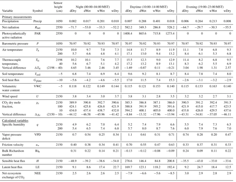
For CO2dry mole fractionχc, we found that above-canopy
χc was largest during wWet conditions and lowest in dDry
conditions with a fairly consistent difference of around 2– 3 µmol mol−1 across the entire diel cycle (Fig. 7a). We
ini-tially considered this to be an artifact of dilution due to boundary layer height differences (e.g., Culf et al., 1997); however, we ruled this out because the difference was fairly consistent throughout the day and night when boundary layer heights change dramatically. We confirmed that sim-ilar χc differences between precipitation states existed
us-ing CO2 measured above tree-line on Niwot Ridge about
3.5 km northwest of the US-NR1 tower (Stephens et al., 2011) (results not shown). Since our analysis uses a com-posite which approximates a cold-front passage, there is an influence of large-scale weather systems on the overall at-mospheric CO2magnitude (e.g., Miles et al., 2012; Lee et al.,
2012). This suggests that the dependence of above-canopyχc
on the precipitation state was due to either the composition
of large-scale air masses or subsidence/convergence caused by high/low barometric pressure.
Within the canopy, this same precipitation-dependent pat-tern existed in the morning and during the daytime, how-ever, in the evening, χc in dry conditions was about 5–
8 µmol mol−1 larger than χ
c in wet conditions (Fig. 7b–
c). These differences clearly show up in a verticalχc
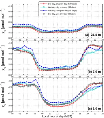
pro-file (Fig. 8c). To avoid the confounding factor of synoptic weather systems, the lower panels in Fig. 8 show the ver-tical χc differences (1χc) relative to the top tower level
(21.5 m a.g.l.). The mid-day 1χc profile (Fig. 8e) shows
a photosynthetic deficit of around 1 µmol mol−1in the
mid-canopy due to vegetative uptake of CO2which is consistent
with previous studies at the site (Bowling et al., 2009; Burns et al., 2011). In the nighttime hours (00:00–04:00 MST) the different precipitation states did not affect the 1χc profile
(Fig. 8d) which contrasts with the late evening1χc profile
that shows a difference of around 5–9 µmol mol−1between
00 02 04 06 08 10 12 14 16 18 20 22 24 380
385 390 395 400 405 410
χ c
[
µ
mol mol
−1
]
(a) 21.5 m Dry day, dry prev day (530 days)
Wet day, dry prev day (83 days) Wet day, wet prev day (46 days) Dry day, wet prev day (82 days)
00 02 04 06 08 10 12 14 16 18 20 22 24
380 385 390 395 400 405 410
χ c
[
µ
mol mol
−1
]
(b) 7.0 m
00 02 04 06 08 10 12 14 16 18 20 22 24
380 390 400 410 420 430
χ c
[
µ
mol mol
−1
]
(c) 1.0 m
Local hour of day (MST)
Figure 7.The warm-season mean diel cycle of CO2mole fraction
χcat three different heights above the ground. Each line represents a different precipitation state as shown in the legend. These mea-surements are from the warm season in years 2006–2012.
Though synoptic barometric pressure changes have re-cently been suggested as a mechanism for enhancing the ex-change of deep-soil CO2with the atmosphere (e.g.,
Sánchez-Cañete et al., 2013), the larger 1χc differences in dry
conditions are consistent with the near-ground atmospheric stability being larger during dry conditions (discussed in Sect. 3.2.1). Between 00:00 and 04:00 MST Rib was
gen-erally near or above 0.2 for both wet and dry conditions, whereas in the evening period on wet days Rib was≈0.1.
As shown in previous work at the US-NR1 site (e.g., Scha-effer et al., 2008a; Burns et al., 2011),1χcdifferences have
a transition region between weakly stable and strongly stable conditions that occurs at Rib≈0.25 which is nominally
re-lated to the change from a fully turbulent to non-turbulent flow. It appears that the stability in the early evening on wet days is such that the atmosphere was slightly unstable which enhanced the vertical mixing and reduced the verti-cal1χcdifferences. Furthermore, the controls on the
stabil-ity between dWet and wWet days were slightly different. On dWet evenings, wind speed was slightly elevated (Fig. 3d) which resulted in less stable conditions. In contrast, on wWet evenings it was the reduced vertical temperature differences (Fig. 4f) that was the primary controlling factor in reducing the stability.
380 390 400 410 420 430 440 450 0
5 10 15 20
z [m]
(a) 0000 − 0400 MST
0 10 20 30 40 50
0 5 10 15 20
(d)
z [m]
380 390 400 410 420 430 440 450 (b)
χc [µmol mol −1]
1000 − 1400 MST
−2 02 4 6 8 10 12 14 16 18 20
(e)
∆χc [µmol mol −1]
380 390 400 410 420 430 440 450 (c) 1900 − 2300 MST
0 10 20 30 40 50
(f) Dry day, dry previous day
Wet day, dry previous day Wet day, wet previous day Dry day, wet previous day
Figure 8. Mean vertical profiles of CO2 mole fraction χc for (left) nighttime (00:00–04:00 MST), (middle) mid-day (10:00– 14:00 MST), and (right) late evening (19:00–23:00 MST). The up-per row is absoluteχc while the bottom row is theχc difference relative to the highest level (21.5 m). Each line represents a differ-ent precipitation state as shown in the legend. These measuremdiffer-ents are from the warm season in years 2006–2012.
3.2.4 Net radiation and turbulent energy fluxes
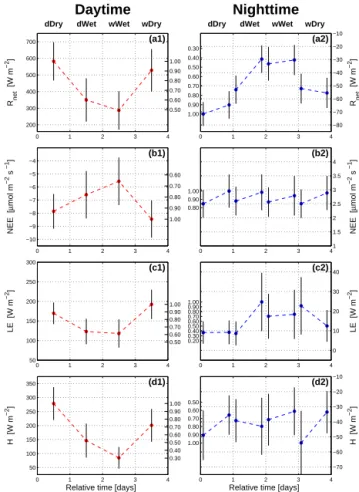
The full diel cycle of net radiation, the turbulent energy fluxes, NEE, and transpiration are shown in Fig. 9 where the diel cycles are arranged by dDry, dWet, wWet, and wDry conditions. The dDry conditions are repeated in each column to make comparison between conditions easier. In order to better quantify the impact of precipitation state on the fluxes, we also show a summary that only includes mean mid-day (Fig. 10, left-column) and late evening and nighttime values (Fig. 10, right-column). To make interpretation of the quan-titative changes more accessible, each panel in Fig. 10 shows the fractional change from the maximum (or minimum) value within that panel. The mean values for each precipitation state are also listed in Table 3.
When precipitation occurred, cloudiness increased and net radiation at mid-day was reduced (Fig. 9a). dDry days had a mean mid-day value of nearly 600 W m−2which decreased
by around 50 % to 300 W m−2 during wWet days, then
re-covered on wDry days to nearly 550 W m−2(i.e., about 10 %
−100 0 100 200 300 400 500 600 Rnet [W m −2 ] (a)
dDry dWet wWet wDry
−200 0 200 400 600 800 1000 1200 (Q sw ↓ ) TOA [W m −2 ]
0 4 8 12 16 20 24 4 8 12 16 20 24 4 8 12 16 20 24 4 8 12 16 20 24
−10 −8 −6 −4 −2 0 2 4
NEE [
µ mol m −2 s −1 ] (b)
0 4 8 12 16 20 24 4 8 12 16 20 24 4 8 12 16 20 24 4 8 12 16 20 24
0 40 80 120 160 200
LE [W m
−2
]
(c)
0 4 8 12 16 20 24 4 8 12 16 20 24 4 8 12 16 20 24 4 8 12 16 20 24
−100 −50 0 50 100 150 200 250 300
H [W m
−2
]
(d)
0 4 8 12 16 20 24 4 8 12 16 20 24 4 8 12 16 20 24 4 8 12 16 20 24
0 0.2 0.4 0.6 0.8 1
Transpiration [relative]
(e)
Local hour of day (MST)
Figure 9. The mean warm-season diel cycle of(a)net radiation
Rnet,(b)net ecosystem exchange of CO2NEE,(c)latent heat flux
LE,(d)sensible heat fluxH, and(e)transpiration (in relative units).
The diel cycle for each precipitation states are shifted to the right following the description above panel(a). For reference, the dDry
diel cycle is repeated in all columns as a red line. In(a),
incom-ing shortwave radiation at the top of the atmosphere (Q↓SW)TOA is shown as a black line in the dDry column (using the right-hand axis). Transpiration is estimated from several pine trees near the US-NR1 tower during the summers of 2004, 2006, and 2007. For all other variables, the diel cycle is calculated from 30 min mea-surements between years 1999 and 2012.
At night, though the absolute value of the mean net radi-ation was an order of magnitude smaller than the daytime values, the fractional changes and pattern of nocturnal Rnet
due to different precipitation states (Fig. 10a2) were simi-lar to those of mid-day Rnet (Fig. 10a1). If we assume that
wet nights were cloudier than dry nights, the radiative sur-face cooling on clear nights was around−70 W m−2, while
that of cloudy nights was closer to−30 W m−2. The
reduc-0 1 2 3 4
200 300 400 500 600 700 Daytime dDry dWet wWet wDry
Rnet [W m −2 ] 1.00 0.90 0.80 0.70 0.60 0.50 (a1)
0 1 2 3 4
−80 −70 −60 −50 −40 −30 −20 −10 Rnet [W m −2 ] Nighttime dDry dWet wWet wDry
1.00 0.90 0.80 0.70 0.60 0.50 0.40 0.30 (a2)
0 1 2 3 4
−10 −9 −8 −7 −6 −5 −4
NEE [
µ mol m −2 s −1 ] 1.00 0.90 0.80 0.70 0.60 (b1)
0 1 2 3 41
1.5 2 2.5 3 3.5 4
NEE [
µ mol m −2 s −1 ] 1.00 0.90 0.80 (b2)
0 1 2 3 4
50 100 150 200 250 300
LE [W m
−2 ] 1.00 0.90 0.80 0.70 0.60 0.50 (c1)
0 1 2 3 4
0 10 20 30 40
LE [W m
−2 ] 1.00 0.90 0.80 0.70 0.60 0.50 0.40 0.30 0.20 (c2)
0 1 2 3 4
50 100 150 200 250 300 350
Relative time [days]
H [W m
−2 ] 1.00 0.90 0.80 0.70 0.60 0.50 0.40 0.30 (d1)
0 1 2 3 4
−70 −60 −50 −40 −30 −20 −10
Relative time [days]
H [W m
−2 ] 1.00 0.90 0.80 0.70 0.60 0.50 (d2)
Figure 10. Mean values for (left column) daytime (10:00–
14:00 MST) and (right column) night (00:00–04:00 MST) and evening (19:00–23:00 MST) periods of(a1, a2)net radiationRnet;
(b1, b2)net ecosystem exchange of CO2NEE;(c1, c2)latent heat
flux LE; and(d1, d2)sensible heat fluxH. The values are arranged from left-to-right in the order of dDry, dWet, wWet, and wDry con-ditions. The vertical black lines represent the mean absolute de-viation (MAD) of the 30 min data within that particular category and time period. The numerical values shown between the daytime and nighttime panels represent the fractional change relative to the largest (or smallest) data value within the panel.
tion of the magnitude ofRneton wet nights was primarily due
to changes in cloud cover as well as changes to the turbulent fluxes.
Sensible heat flux during mid-day had a similar pattern to net radiation, with a large decrease in H (by ≈70 %)
between dDry and wWet conditions, followed by a return toward dDry H on wDry days (Fig. 10d1). In contrast,
la-tent heat flux followed a different pattern – the largest mean mid-day LE occurred on a wDry day with a value of around 200 W m−2, which was around 15 % larger than mid-day LE
on dDry days (Figs. 9c, 10c1). The extra energy used by LE (coupled with slightly lowerRnetvalues on wDry days)
ex-plains why mid-dayH only recovered to within 80 W m−2
(or 30 %) of dDryH as dictated by the SEB (Eq. 1) and
0 0.5 1 1.5 2 2.5 0 100 200 300 400 (b1)
dDry LE [W m
−2
]
1000−1400 MST
0 0.5 1 1.5 2 2.5
0 100 200 300 400 (b2)
dWet LE [W m
−2
]
0 0.5 1 1.5 2 2.5
0 100 200 300 400 (b3)
wWet LE [W m
−2
]
Rnet > 600 W m−2 Rnet < 600 W m−2
0 0.5 1 1.5 2 2.5
0 100 200 300 400 (b4)
wDry LE [W m
−2
]
VPD [kPa]
0 0.5 1 1.5 2 2.5
0 10 20 30 40 50 60
LE [W m
−2
]
(a1) 0000−0400 MST dDry: Dry day, dry previous day dWet: Wet day, dry previous day wWet: Wet day, wet previous day wDry: Dry day, wet previous day
0 0.5 1 1.5 2 2.5
0 50 100 150 200 250 300 350
(a2) 1000−1400 MST
<−−− (wDry − dDry)
LE [W m
−2
]
Pine
Spruce
0 5 10 15 20 25 30 35
Transpiration [g H
2
O cm
−2
day
−1
]
0 0.5 1 1.5 2 2.5
0 10 20 30 40 50 60
(a3) 1900−2300 MST
VPD [kPa]
LE [W m
−2
]
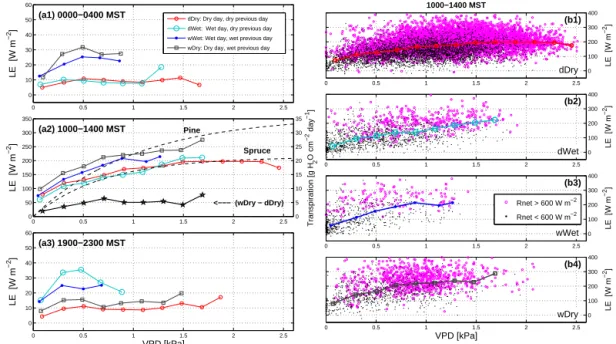
Figure 11.The (left column) binned 21.5 m latent heat flux LE vs. 21.5 m vapor pressure deficit VPD for(a1)night (00:00–04:00 MST), (a2)daytime (10:00–14:00 MST), and(a3)evening (19:00–23:00 MST) periods. Each line represents a different precipitation state as shown in the legend. In(a2), the dashed black lines are the empirical exponential fits of transpiration per unit sapwood area vs. VPD for 2006 as
determined by Hu et al. (2010b) for pine and spruce trees (using the right-hand axis). Also, the difference in LE between wDry and dDry conditions is shown as a solid black line. As an example of the variability in the binned data, the right-column panels show the 30 min daytime data used to create the binned daytime lines (i.e., corresponding to what is shown in panela2). The right-column panels are for (b1)dDry,(b2)dWet,(b3)wWet, and(b4)wDry periods. In the scatter plots, the individual points are distinguished byRnetas shown by the legend in(b3).
At night, latent heat flux cooled the surface and was strongly affected by changes in the precipitation state (Fig. 10c2) following a pattern similar to that of nocturnal
Rnet (Fig. 10a2). Nocturnal sensible heat flux changed by
around 30–40 % during the different precipitation states, but the pattern did not clearly follow that of either Rnet or LE
(Fig. 10d2). At night, H generally warms the surface
(in-cluding the forest vegetation and other biomass) following the air-surface temperature gradient (i.e., similar to the ver-tical temperature differences shown in Fig. 4d and f). In this way,Hacts to compensate for air-surface temperature
differ-ences that might be generated by the surface cooling effects ofRnetand LE. Even though the vertical air temperature
dif-ferences were largest during dDry conditions (Fig. 4d and f) the largest sensible heat flux occurred during wDry periods between 00:00–04:00 MST (Fig. 10d2). This is exactly when LE was at a maximum (so evaporative cooling would be ex-pected) and a close look at Fig. 4f reveals that the temper-ature difference between the air just above the ground and soil was larger in wDry conditions than dDry conditions. We should also note that what is shown in Fig. 4d and f are ver-tical air temperature differences which serve as a surrogate for the actual difference between air temperature and the sur-face elements (i.e., tree branches, needles, boles, and the soil surface) (e.g., Froelich et al., 2011).
3.2.5 The evaporative contribution to LE
The increased LE values on wDry days was presumably due to evaporation of the intercepted liquid water present on veg-etation and in the soil. Because of the effect of temperature on saturation vapor pressure (and thus VPD) one cannot as-sume outright that nocturnal LE is representative of daytime evaporation (e.g., Brutsaert, 1982). To further explore this is-sue, we have plotted LE vs. VPD in Fig. 11 where we observe that nocturnal LE in dry conditions was ≈10 W m−2 with
a weak dependence on VPD. The trend toward less evap-oration in dDry conditions is due to a large soil resistance to evaporation when the soil/litter surface under a canopy is dry (Baldocchi and Meyers, 1991). This is consistent with there being a small, persistent baseline level of evaporation in dry conditions and we make an assumption that this level of evaporation is similar during the daytime. Therefore, in dDry conditions we can estimate that evaporation was≈10 W m−2
and evapotranspiration was≈170 W m−2(based on mid-day