Prediction of future hydrological regimes in poorly gauged high altitude basins: the case study of the upper Indus, Pakistan

(1)

HESSD

8, 3743–3791, 2011

Prediction of future hydrological regimes

in the upper Indus

D. Bocchiola et al.

Title Page

Abstract Introduction

Conclusions References

Tables Figures

◭ ◮

Back Close

Full Screen / Esc

Printer-friendly Version Interactive Discussion

Discussion

P

a

per

|

Dis

cussion

P

a

per

|

Discussion

P

a

per

|

Discussio

n

P

a

per

|

Hydrol. Earth Syst. Sci. Discuss., 8, 3743–3791, 2011 www.hydrol-earth-syst-sci-discuss.net/8/3743/2011/ doi:10.5194/hessd-8-3743-2011

Hydrology and Earth System Sciences Discussions

This discussion paper is/has been under review for the journal Hydrology and Earth System Sciences (HESS). Please refer to the corresponding final paper in HESS if available.

Prediction of future hydrological regimes

in poorly gauged high altitude basins: the

case study of the upper Indus, Pakistan

D. Bocchiola1, G. Diolaiuti2, A. Soncini1, C. Mihalcea2, C. D’Agata2, C. Mayer3, A. Lambrecht3, R. Rosso1, and C. Smiraglia2

1

Dept. Hydrologic, Environmental, Roads and Surveying Engineering, Politecnico di Milano, L. Da Vinci, 32, 20133, Milano, Italy

2

Dept. Earth Sciences, Universit `a di Milano, Mangiagalli, 34, 20133, Milano, Italy 3

Commission for Glaciology, Bavarian Academy of Sciences, A. Goppel, 11, 80539 Munich, Germany

Received: 13 April 2011 – Accepted: 13 April 2011 – Published: 15 April 2011

Correspondence to: D. Bocchiola (daniele.bocchiola@polimi.it)

(2)

HESSD

8, 3743–3791, 2011

D. Bocchiola et al.

Title Page

Tables Figures

◭ ◮

Back Close

Full Screen / Esc

Discussion

P

a

per

|

Dis

cussion

P

a

per

|

Discussion

P

a

per

|

Discussio

n

P

a

per

|

Abstract

In the mountain regions of the Hindu Kush, Karakoram and Himalaya (HKH) the “third polar ice cap” of our planet, glaciers play the role of “water towers” by providing sig-nificant amount of melt water, especially in the dry season, essential for agriculture, drinking purposes, and hydropower production. Recently, most glaciers in the HKH

5

have been retreating and losing mass, mainly due to significant regional warming, thus calling for assessment of future water resources availability for populations down slope. However, hydrology of these high altitude catchments is poorly studied and little understood. Most such catchments are poorly gauged, thus posing major issues in flow prediction therein, and representing in facts typical grounds of application of PUB

10

concepts, where simple and portable hydrological modeling based upon scarce data amount is necessary for water budget estimation, and prediction under climate change conditions. In this preliminarily study, future (2060) hydrological flows in a particular watershed (Shigar river at Shigar, ca. 7000 km2), nested within the upper Indus basin and fed by seasonal melt from major glaciers, are investigated.

15

The study is carried out under the umbrella of the SHARE-Paprika project, aiming at evaluating the impact of climate change upon hydrology of the upper Indus river. We set up a minimal hydrological model, tuned against a short series of observed ground climatic data from a number of stations in the area, in situ measured ice ablation data, and remotely sensed snow cover data. The future, locally adjusted, precipitation and

20

temperature fields for the reference decade 2050–2059 from CCSM3 model, available within the IPCC’s panel, are then fed to the hydrological model. We adopt four different glaciers’ cover scenarios, to test sensitivity to decreased glacierized areas. The pro-jected flow duration curves, and some selected flow descriptors are evaluated. The un-certainty of the results is then addressed, and use of the model for nearby catchments

25

(3)

HESSD

8, 3743–3791, 2011

D. Bocchiola et al.

Title Page

Tables Figures

◭ ◮

Back Close

Full Screen / Esc

Discussion

P

a

per

|

Dis

cussion

P

a

per

|

Discussion

P

a

per

|

Discussio

n

P

a

per

|

1 Introduction

The mountain range of the Hindu Kush, Karakoram and Himalaya (HKH) contains a large amount of glacier ice, and it is thethird pole of our planet (e.g. Smiraglia et al., 2007; Kehrwald et al., 2008), delivering water for agriculture, drinking purposes and power production. There are estimates indicating that more than 50% of the water

5

flowing in the Indus river, Pakistan, which originates from the Karakoram, is due to snow and glacier melt (Immerzeel et al., 2010). The hydrological regimes of HKH rivers and potential impact of climate change therein have been hitherto assessed in a number of contribution in the scientific available literature (e.g. Aizen et al., 2002; Hannah et al., 2005; Kaser et al., 2010).

10

Economy of Himalayan regions is relying upon agriculture, and thus is highly de-pendent on water availability and irrigation systems (e.g. Akhtar et al., 2008). The Indo-Gangetic plain (IGP, including regions of Pakistan, India, Nepal, and Bangladesh) is challenged by increasing food production in line with demand grows ever greater, and any perturbation in agriculture will considerably affect the food systems of the

re-15

gion and increase the vulnerability of the resource-poor population (e.g. Aggarwal et al., 2004; Kahlown et al., 2007).

Nepal and northern India experience monsoonal floods during late summer (July– September), whereas in winter season (December–February) they display very low flows, terribly impacting agriculture.

20

The human settlements within HKH are tightly bound for their survival to agricul-ture, including wheat and more important sources of food integration (e.g. orchards, potato, tomato, Weiers, 1995). Agricultural irrigation in Pakistan rely heavily upon use of groundwater, and most of groundwater recharge is made up by irrigation wa-ter losses, with rainfall providing only some 10%. Due to high evapotranspiration (ET)

25

(4)

HESSD

8, 3743–3791, 2011

D. Bocchiola et al.

Title Page

Tables Figures

◭ ◮

Back Close

Full Screen / Esc

Discussion

P

a

per

|

Dis

cussion

P

a

per

|

Discussion

P

a

per

|

Discussio

n

P

a

per

|

The HKH stores a very relevant amount of water in its extensive glacier cover at higher altitudes (about 16 300 km2), but the lower reaches are very dry. Especially in the Central and Northern Karakoram, the lower elevations receive only occasional rain-fall during summer and winter (e.g. Winiger et al., 2005). The state of the glaciers also plays an important role in future planning: shrinking glaciers may initially provide more

5

melt water, but later their amount may reduced; on the other hand, growing glaciers store precipitation, reduce summer runoff, and can also generate local hazards. These di_fferences could be caused by increases in precipitation since the 1960s (Archer and Fowler, 2004) and a simultaneous trend toward higher winter temperatures and lower summer temperatures (Fowler and Archer, 2005).

10

As such, climate change represent a main source of risk for floods and for thefood securityof the populations living within the area of HKH. In view of the dramatic impor-tance of this issue and the consideration it deserves nowadays from the international scientific community, the number of studies assessing the impact of climate change for the Alpine area, particularly in the Italian Alps, seems still limited. Maybe less

devel-15

oped seems the assessment of water resources for the HKH region. Long term mea-surements of hydrological and climatologic data of the highest glacierized areas are seldom available (see Chalise et al., 2003), thus making assessment of hydro-climatic trends difficult to say the least.

Recent studies indicate that glaciers of south-eastern Tibet have negative mass

bal-20

ances (Aizen and Aizen, 1994). Ageta and Kadota (1992) suggested that small glaciers in the Nepal Himalaya and Tibetan Plateau would disappear in a few decades if air temperature persistently exceeds a few degrees above that required for an equilib-rium state of mass balance. Moreover very recently time air pollution and in particular atmospheric soot seem to affect Himalayan glacier albedo, increasing ice and snow

25

(5)

HESSD

8, 3743–3791, 2011

D. Bocchiola et al.

Title Page

Tables Figures

◭ ◮

Back Close

Full Screen / Esc

Discussion

P

a

per

|

Dis

cussion

P

a

per

|

Discussion

P

a

per

|

Discussio

n

P

a

per

|

Akhtar et al. (2008) investigated hydrological conditions pending different climate change scenarios (PRECIS model, A2 storyline) for three glacierized watersheds in the Hindukush-Karakoram-Himalaya (Hunza, 13 925 km2, glacierized 4688 km2; Gilgit, 12800 km2, glacierized 915 km2; Astore, 3750 km2, glacierized 612 km2). Their results indicate temperature and precipitation increase towards the end of 21st century, with

5

discharges increasing for 100% and 50% glacier cover scenarios, whereas noticeable decrease is conjectured for 0% scenario, i.e. for depletion of ice caps. Albeit the authors stress low quality of the observed data, they claim transfer of climate change signals into hydrological changes is consistent.

Immerzeel et al. (2009) used remotely sensed precipitation (from TRMM) and snow

10

covered area SCA (from MODIS®), together with ground temperature data and a sim-ple Snow Melt RunoffModel (SRM), to calibrate an hydrological model and then pro-jected forward in time (PRECIS model, 2071–2100) the hydrological response of the strongly snow fed Indus watershed (Pakistan, NW Himalaya, 200 677 km2, including the Hunza and Gilgit basins). They found warming in all seasons, and greater at the

15

highest altitudes, giving diminished snow fall, whereas total precipitation increases of 20% or so. They found snow melt peaks shifted up to one month earlier, increased glacial flow due to temperature, and significant increase of rainfall runoff.

While southern Himalaya is strongly influenced by the monsoon climate and by abun-dant seasonal precipitation therein, meteo-climatic conditions of Karakoram suggest a

20

stricter dependence of water resources upon snow and ice ablation, and therefore the needs of its believable projection for the future (Mayer et al., 2010). In facts, most high altitude catchments in HKH are not gauged, or only poorly gauged, thus posing major issues in flow prediction therein.

Prediction in ungauged or poorly gauged basins is a tremendously important issue

25

(6)

HESSD

8, 3743–3791, 2011

D. Bocchiola et al.

Title Page

Tables Figures

◭ ◮

Back Close

Full Screen / Esc

Discussion

P

a

per

|

Dis

cussion

P

a

per

|

Discussion

P

a

per

|

Discussio

n

P

a

per

|

to make predictions in areas with poor coverage of hydrological data (Sivapalan et al., 2003; Seibert et al., 2009). High altitude glacierized catchments represent typical grounds of application of PUB concepts, where simple hydrological modeling based upon scarce data amount is necessary for water budget estimation, and prediction un-der climate change conditions (e.g. Chalise et al., 2003; Konz et al., 2007; Immerzeel

5

et al., 2009; Bocchiola et al., 2010). Pillars of PUB initiative and methodology are the concepts of catchment classification (e.g. Burn, 1997; Gabriele et al., 1991; Castellarin et al., 2001; 2008; Parajka et al., 2005; Merz and Bl ¨oschl, 2009) and model portabil-ity (e.g. B ´ardossy, 2007; Buytaert et al., 2008; Castiglioni et al., 2010), basic tools to extrapolate results within measured area to ungauged sites. However, use of such

10

tools require accurate knowledge of physiographic, climatic and hydrologic attributes of some measured catchments within a certain region, and their proper treatment in order to complement analysis of unmeasured areas. Concerning HKH region, albeit some studies have been carried out concerning hydrological similarity (Hannah et al., 2005, for Nepal), and general hydrological regime (e.g. Archer, 2003 for three

catch-15

ments in Karakoram), accurate studies about regional homogeneity and related spatial extent seem yet to come. Nor the required data (weather, hydrology, topography, soil cover, etc.) are easily available and widely spread, especially given the considerable altitude of the contributing catchments, where ice and snow plays a predominant role, and their dynamics is mostly unknown in practice. Upon such ground, development of

20

a generally valid and accurate approach to regional hydrological modeling in this area seems beyond the present know how.

To initiate filling this gap we present here a simple approach to modeling of hydro-logical regime within a high altitude poorly gauged catchment, which illustrates one way to profit of scarce data coming from different sources, and may be of use in other

25

unmeasured catchments of the area.

(7)

HESSD

8, 3743–3791, 2011

D. Bocchiola et al.

Title Page

Tables Figures

◭ ◮

Back Close

Full Screen / Esc

Discussion

P

a

per

|

Dis

cussion

P

a

per

|

Discussion

P

a

per

|

Discussio

n

P

a

per

|

SHARE-Paprika project, funded by the EVK2CMNR committee of Italy, aiming at eval-uating the impact of climate change upon hydrology of the upper Indus river. We set up a minimal hydrological model, tuned against a short series of observed ground climatic data from a number of stations, in situ measured ablation, and remotely sensed snow covered areas. We then feed our model with locally adjusted future, precipitation and

5

temperature fields from the CCSM3 GCM, available within the IPCC’s, using storyline A2, for the reference period 2050–2059. We adopt four different glaciers’ cover scenar-ios, to test runoffsensitivity to decreasing size of glacierized areas. The projected flow duration curves, and some selected flow descriptors are evaluated. We then comment the modified snow cover, ice ablation regime and implications for water resources,

dis-10

playing sensitivity to the chosen scenario. The uncertainty of the results is addressed, and some indications are given about how the simplified approach here proposed could be used to gather knowledge about ungauged catchments in this area.

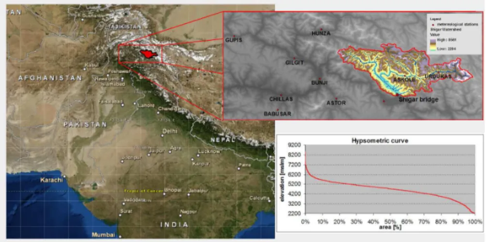
2 Case study area

The study are is in the northern of Pakistan (Fig. 1), in the Hindu Kush, Karakoram

15

and Himalaya (HKH) region, ranging ca. from 74.5◦E to 76.5◦E in Longitude, and from 35.2◦N to 37◦N in Latitude. This preliminary study are been conducted in a particu-lar watershed (Shigar river closed to Shigar bridge, ca. 7000 km2), nested within the upper Indus basin, and fed by seasonal melt from major glaciers. We tackled assess-ment of hydrology within this particular contributor to the Indus river because its whole

20

catchment is laid within Pakistan, whereas a considerable part of the Indus catchment drains the mountain chains of China and India before flowing therein. This makes data retrieval easier, while fitting the purpose of the SHARE-Paprika project, specifically interested into the effect of climate change within the Karakoram range of Pakistan.

The highest altitude here is reached by K2 mountain (8611 m a.s.l.) and the lower is

25

(8)

HESSD

8, 3743–3791, 2011

D. Bocchiola et al.

Title Page

Tables Figures

◭ ◮

Back Close

Full Screen / Esc

Discussion

P

a

per

|

Dis

cussion

P

a

per

|

Discussion

P

a

per

|

Discussio

n

P

a

per

|

(Peel et al., 2007) this area falls in the BWK region, that displays dry climate with by little precipitation and a wide daily temperature range. The HKH area displays consid-erable vertical gradients. The Nanga Parbat massif forms a barrier to the Northward movement of monsoon storms, which intrudes little in Karakoram. In the HKH range there is extensive coverage of glaciers. About 13 000 km2 of glaciers are laid within

5

Pakistan, and in the Shigar basin the main one is the Baltoro, greater than 700 km2 in area. Thus, the hydrological regime is little influenced by monsoon and a major contribution results from snowmelt and glacier melt. Precipitation is concentrated in two main periods, Winter (JFM) and summer (JAS), i.e. Monsoon and Westerlies, the latter providing the dominant nourishment for the glacier systems of the HKH. Some

10

studies indicates that these mountains gain a total annual rainfall between 200 mm and 500 mm, amounts that are generally derived from valley-based stations and less representative for the highest zones (e.g. Archer, 2003). High altitude snowfall seems to be neglected and is still rather unknown. Some estimates from accumulation pits above 4000 m a.s.l. range from 1000 mm to more than 3000 mm, depending on the site

15

(Winiger et al., 2005). However, there is considerable uncertainty about the behavior of precipitation at high altitudes.

3 Database

3.1 Observed data

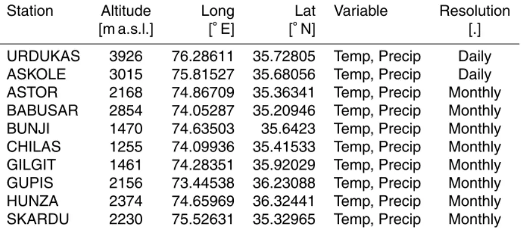
As reported, in the Shigar river catchment we have available data from two

meteoro-20

logical stations, property of the EVK2CNR committee: Askole (3015 m a.s.l.), and Ur-dukas (3926 m a.s.l.). For these stations there are available daily values of rainfall and mean air temperature for the period from 2005 until 2009, but with significant missing data periods, especially for the precipitation. These gaps are concentrated particularly in Winter, likely as precipitation falls under snow form, not measured at these

sta-25

(9)

HESSD

8, 3743–3791, 2011

D. Bocchiola et al.

Title Page

Tables Figures

◭ ◮

Back Close

Full Screen / Esc

Discussion

P

a

per

|

Dis

cussion

P

a

per

|

Discussion

P

a

per

|

Discussio

n

P

a

per

|

precipitation and temperature during 1980–2009, for 8 stations belonging to Pakistan meteorological department, PMD, all positioned below 2500 m a.s.l. Monthly mean dis-charge averaged over the period from 1985 until 1997 are available. During this period there was an hydrometric station property of the water power development agency of Pakistan WAPDA at the Shigar bridge (2204 m a.s.l.), that is our control section (e.g.

5

Archer, 2003). Weather data coverage is summarized in Table 1.

3.2 SCA data

We here used SCA as derived from MODIS® images. Nowadays, SCA estimation from satellite data is widely adopted for water storage assessment in mountain areas, distributed modeling of snow cover and melting and hydrological and glaciological

im-10

plications therein (e.g. Swamy and Brivio, 1996; Simpson et al., 1998; Cagnati et al., 2004; Hauser et al., 2005; Parajka and Bl ¨oschl, 2008; Georgievsky, 2009; Immerzeel et al., 2009). Unsupervised classification of SCA may be carried out based upon visible bands (RGB) andbox typeclassification (Hall et al., 2003a, b, 2010, for estimation of SCA from MODIS® images), using digital number,DN>200.

15

Also sub-pixel classification is used, e.g. by spectral unmixing (e.g. Foppa et al., 2004), which still requires subjective choice of end-members (and more spectral bands for more end-members), while the main output is a percentage of in cell snow cover-age, with no indication of spatial distribution of cells with snow. Here we used 40 images of SCA from MODIS during 2006–2008, taken from the product MODIS/Terra

20

Maximum-Snow Cover 8-Day, L3 Global, at a 500 m resolution (MOD10A2, e.g. Hall et al., 2002). This contains Maximum SCA (yes/no) over an 8-day composing period. As no snow cover data were available within the catchment, as reported, we could not attempt either spatial estimation of snow cover (as e.g. in Bocchiola, 2010; Bocchiola and Groppelli, 2010), or investigation of snowfall properties in the area (e.g. Bocchiola

25

(10)

HESSD

8, 3743–3791, 2011

D. Bocchiola et al.

Title Page

Tables Figures

◭ ◮

Back Close

Full Screen / Esc

Discussion

P

a

per

|

Dis

cussion

P

a

per

|

Discussion

P

a

per

|

Discussio

n

P

a

per

|

3.3 GCM data

We use here the modelNCAR-CCSM3, recently released by the National Centre for Atmospheric Research, in Boulder, Colorado. This model has been included within the 3rd IPCC report (2007) and appears to be more accurate compared with some others

GCMs, e.g. on the Italian Alps (Soncini et al., 2011), and its resolution is comparatively

5

finer with respect to other models.

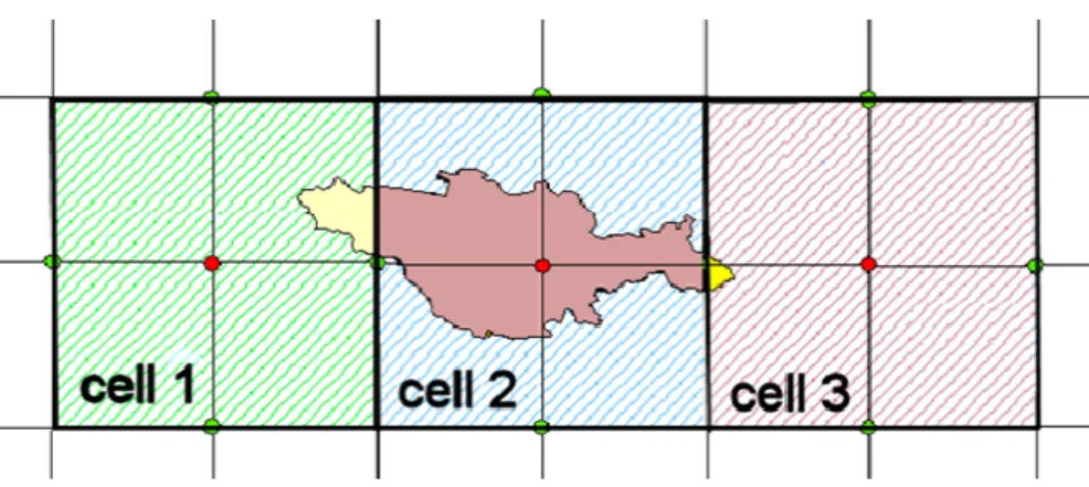
The Shigar basin falls into three cells of the CCSM3 model (Fig. 2, Table 2), albeit mostly contained in the centre one. Here, we evaluate temperature and precipitation within the basin by area weighting. Typically, GCMs provide a bad representation of small scale e_ffects upon precipitation, e.g. topographic control. Therefore, a

downscal-10

ing is necessary (e.g. Ferraris et al., 2003; Groppelli et al., 2011a). Still,GCMs carry considerable information concerning large scale forcing to local climate, so their use is appropriate for projections of climate change impact. The simulations of the GCMs use as input different hypothesis of the future world situation (storylines). A2 storyline is known as “business as usual” and it is most often adopted for climate projections, so

15

we use it here.

4 Methods

4.1 Weather data

To provide input data to our hydrological model for the purpose of testing its perfor-mance we proceed as follows. We use yearly total precipitation from the 8 PMD

sta-20

tions during 1980–2009 (overlapping the period of functioning of the WAPDA hydro-metric station on the Shigar river, 1985–1997) to evaluate the presence and magnitude of altitude lapse rate of temperature and precipitation, and monthly lapse rates were used. Precipitation data show an increase from 1200 m a.s.l. to 3900 m a.s.l. In the absence of further information we adopt a power law (Winiger et al., 2005), which we

25

(11)

HESSD

8, 3743–3791, 2011

D. Bocchiola et al.

Title Page

Tables Figures

◭ ◮

Back Close

Full Screen / Esc

Discussion

P

a

per

|

Dis

cussion

P

a

per

|

Discussion

P

a

per

|

Discussio

n

P

a

per

|

P_y₌9·10−6z2.22, (1)

withPy yearly amount of precipitation [mm] and z is altitude [m a.s.l.]. At high

eleva-tion this may lead to an overestimaeleva-tion of precipitaeleva-tion. However, this may have a little impact on the hydrologic balance, because with increasing altitude contributing area decreases significantly. We preliminarily evaluated the possible presence of an

alti-5

tude lapse rate of precipitation by analyzing maps of average yearly precipitation as derived from TRMM satellite data during 1998–2009 (kindly provided by B. Bookhagen of UCSB, see Bookhagen and Burbank, 2006, 2010) for the Shigar basin area, but we could not detect any clear pattern (not shown for shortness). As a rough comparison, average precipitation in the area could be estimated in ca. 350 mm year−1 by TRMM,

10

whereas use of Eq. (1), tuned as reported using PMD data covering 1980-2009, pro-vided an expected value of ca. 550 mm year−1, i.e. with a difference of 35% or so. However, given the tremendous uncertainty in both techniques, such spread seems not unexpected.

Using the daily precipitation data during 2005–2008 at the Askole station of

15

EVK2CNR, most complete when compared against Urdukas, we then set up a dis-aggregation approach, which we use to disaggregate monthly precipitation from As-tore station (most complete data base among the PMD stations). We use a random cascade approach (e.g. Groppelli et al., 2010, 2011a), slightly modified to deal with monthly precipitation, namely

20

R_d=R_mY_d=R_mB_dW_d P(Bd=0)=1−pd

P(Bd=p

−1

d )=pd

E Bd

=p−_d1pd+0 (1−pd)=1

Wd =e

w_d−σ_wd2 .2

25

E[Wd]=1 ;wd=N

(12)

HESSD

8, 3743–3791, 2011

D. Bocchiola et al.

Title Page

Tables Figures

◭ ◮

Back Close

Full Screen / Esc

Discussion

P

a

per

|

Dis

cussion

P

a

per

|

Discussion

P

a

per

|

Discussio

n

P

a

per

|

whereR_mis monthly rainfall,R_d is daily rainfall, andY_d a daily cascade weight.B_d,p_d, andσ2_wd are model parameters, to be estimated from data, used to preserve intermit-tence, or correct sequence of dry and wet spells. The termBd is aβmodel generator

(e.g. Over and Gupta, 1994). It gives the probability that the rain rateR_d for a given day is non zero, conditioned uponRm being positive, and it is modeled here by a binomial

5

distribution. The termWd is a “strictly positive” generator. It is used to add a proper

amount of variability to precipitation during spells labeled as wet. Model estimation (i.e. estimation ofpd, andσ

2

wd) is pursued monthly, based upon the 2005–2008 series at

Askole. Then, in the hypothesis of similar statistic structure of precipitation between Askole and Astore we use the same approach to downscale monthly precipitation in

10

Astore. So doing, we obtain a daily precipitation series at Astore, which we subse-quently use for hydrological simulation during 1985–1997. Similarly, we use Askole daily temperature data, to disaggregate Astore monthly data, by random extraction of daily temperature according to a given (normal) distribution, estimated from data.

4.2 Ice melt

15

Shigar watershed includes glaciers spread over an area of ca. 4240 km2, several of which displaying debris cover. Mihalcea et al. (2006) and Mayer et al. (2006) evaluate ice melt factors for both ice covered and ice free glacier based upon field ablation data from the Baltoro glacier, and Mayer et al. (2010) evaluated melt factors for Bagrot valley, and Hinarche glacier. Mihalcea et al. (2008) provided evaluation of debris cover

20

(13)

HESSD

8, 3743–3791, 2011

D. Bocchiola et al.

Title Page

Tables Figures

◭ ◮

Back Close

Full Screen / Esc

Discussion

P

a

per

|

Dis

cussion

P

a

per

|

Discussion

P

a

per

|

Discussio

n

P

a

per

|

4.3 Snow melt and SCA

Snow melt was tackled using degree day approach and melt factor. Among others, Singh et al. (2000) provide a review of plausible values for snow melt factors, in-cluding for glaciers in western Himalaya. Melt factors range from 1 mm◦C−1day−1 to 14 mm◦C−1day−1or so. Snow cover data (and subsequent ablation) were not

avail-5

able here, so we tackled estimation of melt factors indirectly. We used our hydrologi-cal model to simulate snow cover at different altitudes for different values of the melt factors, during years 2005–2008, when weather data from EVK2CNR stations were available, and also MODIS SCA data could be retrieved. We then compared the esti-mated snow cover depth, or snow water equivalent SWE (including no snow) against

10

SCA given by MODIS images for 2006–2008. Year 2005 was not considered, because no information about snowfall during the antecedent Fall was available to be used as a boundary conditions. We then estimated a best value for the snow melt factor, as the one providing the best correspondence in term of SCA variation, and snow depletion period.

15

4.4 The hydrological model

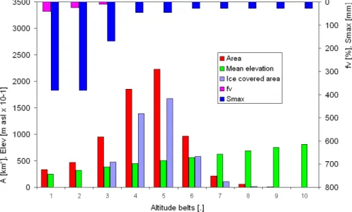
We use a semi-distributed altitude belts based model (Fig. 3), able to reproduce de-position of snow and ablation of both ice and snow, evapotranspiration, recharge of groundwater reservoir, discharge formation and routing to the control section (Grop-pelli et al., 2011b, c). This simple model needs a few input data, i.e. a DEM, daily

20

values of precipitation and temperature, information about soil use, vertical gradient of temperature and precipitation and some others parameters. The model is a simplified version of model DHM, Distributed Hydrological Model (Wigmosta et al., 1994; Chen et al., 2005). In this model are considered two mechanism of flow formation: superficial and groundwater. The model is based on mass conservation equation and evaluates

25

(14)

HESSD

8, 3743–3791, 2011

D. Bocchiola et al.

Title Page

Tables Figures

◭ ◮

Back Close

Full Screen / Esc

Discussion

P

a

per

|

Dis

cussion

P

a

per

|

Discussion

P

a

per

|

Discussio

n

P

a

per

|

St+∆t=St+R+Ms+Mi−ETeff−Qg, (3)

withR the liquid rain, Ms snowmelt, Mi glacial ablation, ETeff the effective

evapotran-spiration, and Q_g groundwater discharge. Snowmelt M_s and glacial ablation M_i are estimated according to a degree day method

Ms=DDs(T−Tt),

5

Mi=DDi(T−Tt), (4)

withT daily mean temperature,DDsandDDimelt factors, evaluated as reported above, andT_tthreshold temperature,T_t=0◦C (Bocchiola et al., 2010). Degree day plus melt factor is a simple and parsimonious method for assessment of ablation and floods in mountain catchments, and it is used here accordingly (Singh et al., 2000; Hock,

10

2003; Simaityte et al., 2008). Ice melt occurs upon glacier covered area within each belt (Fig. 3), after snow depletion is complete. The superficial flowQs occurs only for

saturated soil

Q_s=St+∆t−S_Max if St+∆t> S_Max

Q_s=0 if St+∆t≤ S_Max (5)

with SMax greatest potential soil storage [mm]. Potential evapotranspiration is

calcu-15

lated using Hargreaves equation, only requiring temperature data and monthly mean temperature excursion

ETP=0.0023S0 q

DTm(T+17.8), (6)

in mmd−1, where S0 [mmd

−1

] is the evaporating power of solar radiation (depending upon Julian date and local coordinates), and DTm [

◦

C] is the thermometric monthly

20

(15)

HESSD

8, 3743–3791, 2011

D. Bocchiola et al.

Title Page

Tables Figures

◭ ◮

Back Close

Full Screen / Esc

Discussion

P

a

per

|

Dis

cussion

P

a

per

|

Discussion

P

a

per

|

Discussio

n

P

a

per

|

coefficientsα andβ, depending on the state of soil moisture (water content,θ, given by S/SMax) and from the fraction of vegetated soil (fv) upon the surface of the basin

(see e.g. Brutsaert, 2005; Chen et al., 2005)

E s=α(θ) ETP (1−f_v)

T s=β(θ) ETPfv (7)

5

with

α(θ) =0.082θ₊9.173θ2−9.815θ3

β(θ) = θ−θw θl −θw

if θ > θ_w

β(θ)=0 if θ ≤θ_w (8)

whereθ_wis wilting point water content, whileθ_l is water content at field capacity. Actual

10

evapotranspiration is then

ETeff=E s+T s. (9)

Groundwater discharge is here simply expressed as a function of soil hydraulic con-ductivity and water content (see e.g. Chen et al., 2005)

Qg=K

S SMax

k

, (10)

15

with K saturated permeability and k power exponent. Equations (3–10) are solved using ten equally spaced elevation belts inside the basin. The flow discharges from the belts are routed to the outlet section through a semi-distributed flow routing algo-rithm. This algorithm is based upon the conceptual model of the instantaneous unit hydrograph, IUH (e.g. Rosso, 1984). For calculation of the in stream discharge we

20

(16)

HESSD

8, 3743–3791, 2011

D. Bocchiola et al.

Title Page

Tables Figures

◭ ◮

Back Close

Full Screen / Esc

Discussion

P

a

per

|

Dis

cussion

P

a

per

|

Discussion

P

a

per

|

Discussio

n

P

a

per

|

possesses a time constant (i.e.k_g, k_s). We assumed that for every belt the lag time grows proportionally to the altitude jump to the outlet section, until the greatest lag time (i.e.Tlag,g=ngkg for the groundwater system andTlag,s=nsks for the overland system).

So doing, each belt possesses different lag times (and the farther belts the greater lag times).

5

The hydrological model uses a daily series of precipitation and temperature from one representative station, here Askole, and the estimated vertical gradients to project those variables at each altitude belt. Topography is here represented by a DTM model, with 500 m spatial resolution, derived from ASTER (2006) mission, used to define alti-tude belts and local weather variables against altialti-tude.

10

4.5 Hydrological model calibration

As reported above, we synthetically simulated daily series of temperature and precipi-tation for 1985–1997 by disaggregation of monthly values. We feed these data to our model, to obtain daily estimates of in channel discharge at Shigar bridge. We subse-quently evaluate monthly mean discharges, which we then average during 1985–1997.

15

So doing, we can compare mean monthly simulated discharges against their observed counterparts. As reported, discharge under this form is only available to us. When-ever daily, or monthly discharges for the area would be made available to us, we could compare those path wise against model simulated discharges.

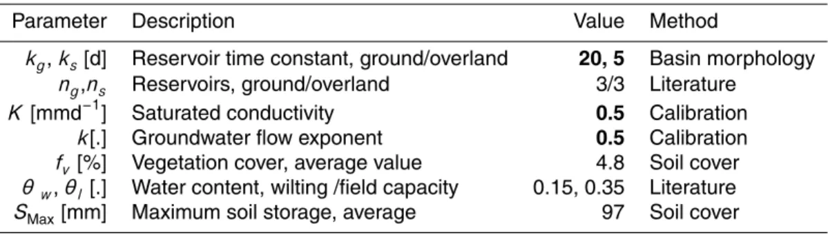
In Table 3 they are specified the parameters that were effectively used for the

cali-20

bration, and those that were estimated on the basis of preliminary considerations and of the analysis of the available literature. Among the model parameters, the value of SMaxis of considerable interest, since it drives the production of overland flow. If one compares this parameter to the parameter S of the method SCS-CN, which possesses the analogous meaning of maximum soil storage, it is possible to estimate in the first

25

(17)

HESSD

8, 3743–3791, 2011

D. Bocchiola et al.

Title Page

Tables Figures

◭ ◮

Back Close

Full Screen / Esc

Discussion

P

a

per

|

Dis

cussion

P

a

per

|

Discussion

P

a

per

|

Discussio

n

P

a

per

|

geological maps (on a paper support) allowed us to define reasonable CN values for each belt, thus making it possible to evaluateSMax.

The wilting point for the (scarce) vegetated areasθw=0.15 was chosen based upon

available references (Chen et al., 2005; Wang et al., 2009). The field capacity was set toθl=0.35, using an average value for mixed grounds, according to studies on a wide

5

range of soils (e.g. Ceres et al., 2009).

Often the number of reservoirs in the overland flow phase depends on the morphol-ogy of the basin, expressed e.g. through morphometric indexes (e.g. Rosso, 1984). However, an analysis of the values observed within several studies indicates an av-erage value of n_s=3, which we use here. In analogy, the number of groundwater

10

reservoirs may be linked to the topography, and we setng=3. A greater variability is

instead necessary for the appraisal of the time constants ks, kg, that define the lag

time of the catchment, and are linked in some way to its size and to the characteristic flow velocity (e.g. Bocchiola et al., 2004; Bocchiola and Rosso, 2009).

We tuned the remaining parameters (see Table 3) with attention to two main goals:

15

accuracy of the yearly average discharge and best fitting to the observed monthly mean series (least sum of percentage squared errors, MSE_%).

We estimated the values of ks and kg by minimizing MSE% (as they do not affect mean yearly discharge). However, while these values do influence flow modeling at the daily scale, at a monthly scale we saw little sensitivity.

20

The saturated permeability valueK=0.5 mmd−1 is consistent with the available lit-erature for a range wide of observed soils, where values between 0.1 mmd−1 and 10 mmd−1 are found (e.g. Timlin et al., 1999; Wang et al., 2009). This parameter has substantial importance during periods of low flows. Here we found that the assump-tion of ground flow linearly dependent against water content (k=1) was not accurate.

25

(18)

HESSD

8, 3743–3791, 2011

D. Bocchiola et al.

Title Page

Tables Figures

◭ ◮

Back Close

Full Screen / Esc

Discussion

P

a

per

|

Dis

cussion

P

a

per

|

Discussion

P

a

per

|

Discussio

n

P

a

per

|

4.6 GCMs downscaling

To evaluate prospective hydrological cycle of the Shigar River, we downscale CCSM3 models’ outputs of precipitation and temperature. Again, a random cascade approach (e.g. Groppelli et al., 2011a) is used to obtain ground precipitation at dayi

Ri=RCCSM3,iYi=RCCSM3,iBiWi

5

P(Bi=0)=1−pi

P(Bi=p

−1

i )=pi

E[B_i]=p−1

i pi+0 (1−pi)=1

Wi =e

w_i−σ2_wi.2

E[W_i]=1 ;w_i=N0,σ_i2 (11)

10

with RCCSM3,i projected CCSM3 precipitation at day i, and cascade model symbols

having the same meaning as in Eq. (2). Again, model setup is carried out using data at Askole station (Table 1) during 2005–2008, and lapse rate as from Eq. (1) used to carry out altitude correction. Downscaling of temperature is also carried out using data at Askole station. We used in practice a monthly averaged DT approach and vertical

15

lapse rate as deduced before to project temperature at each belt.

4.7 Hydrological projections

We feed CCSM3 downscaled climate projections to the calibrated hydrological model. We consider the decade 2050–2059 for comparison against our control period of 13 yr 1985–1997. To project forward hydrology of the area, one needs some

assump-20

(19)

HESSD

8, 3743–3791, 2011

D. Bocchiola et al.

Title Page

Tables Figures

◭ ◮

Back Close

Full Screen / Esc

Discussion

P

a

per

|

Dis

cussion

P

a

per

|

Discussion

P

a

per

|

Discussio

n

P

a

per

|

during 2050–2059, and (iv)−50% ice cover during 2050–2059. To do so we reduce

glaciers’ area moving from the lowest glacierized altitudes towards the highest one, until the proper reduction is obtained.

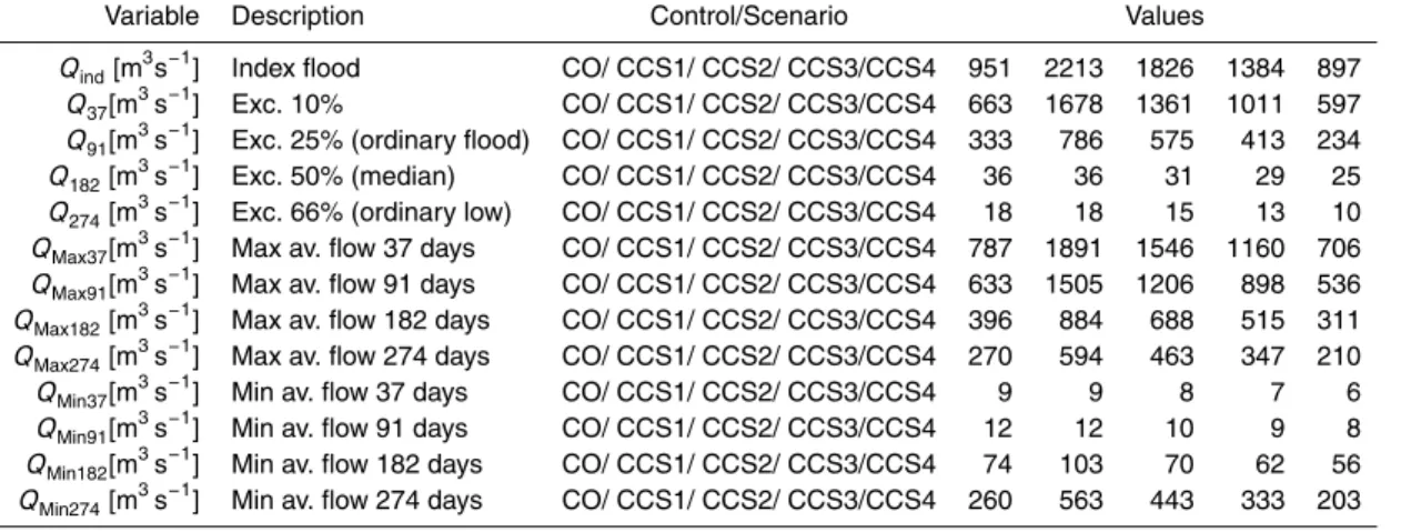
We then calculate a number of flow indicators. First, we calculate flow duration curves, hereon FDCs (e.g. Smakhtin, 2001). FDCs provide visual assessment of the

5

duration of periods (number of days) with discharge above given values, of interest for water resources management as well as for evaluation of ecological effect of flows (e.g. Clausen and Biggs, 2000; Dankers and Feyen, 2008). Also we draw some flow descriptors taken by the FDCs (e.g. Smakthin, 2001), namely the values of flow dis-charges equalled or exceeded for a given number of days, d, i.e. Qd. We consider

10

Q₃₇, or flow exceeded for 10% of the time,Q₉₁, 25% of the time, also known as ordi-nary flood,Q182, i.e. median flow, andQ274, also known as ordinary low flow. Also, we evaluate some flow frequency descriptors given by the yearly minima and maxima of average flows for a given durationd, i.e.Q_Max_d andQ_Min_d. Analysis of these variables is used to pursue statistical appraisal of low flows, e.g. for hydrological drought hazard

15

analysis (e.g. Smakhtin, 2001). In Table 5 we report the average of the yearly values of Q_Max_d andQ_Min_d, ford=37, 91, 182, and 274 days. These values provide the spread between the greatest and least flows expected within the Shigar river for increasingly longer periods.

5 Results

20

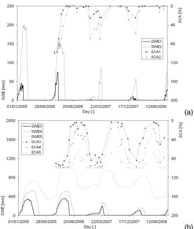
5.1 Snow cover

Figure 4 reports snow cover as simulated by the model during 2005–2008, by setting DDs=2.5 mm

◦

C−1day−1, and MODIS SCA (%) during 2006-2008. We considered alti-tude belts 1 to 5 (i.e. until 5375 m a.s.l.), where most of the snow cover variation occurs (whereas at higher altitudes permanent full snow cover was in practice labeled by both

25

(20)

HESSD

8, 3743–3791, 2011

D. Bocchiola et al.

Title Page

Tables Figures

◭ ◮

Back Close

Full Screen / Esc

Discussion

P

a

per

|

Dis

cussion

P

a

per

|

Discussion

P

a

per

|

Discussio

n

P

a

per

|

days, so daily comparison is approximate. Our comparative analysis indicates a visible correspondence between snowpack SWE as simulated by the model and SCA, indicat-ing synchronous patterns (either increase or decrease). Albeit an indication of non null SCA cannot be translated directly into an estimated value of SWE on the ground, one can guess that decreasing SWE within a given altitude belts implies decreased SCA,

5

and the vice versa for increasing SWE. Therefore, a synchronous pattern as reported indicates proper model functioning. Further on, when SCA moves towards low values (i.e. close to zero) the modeled SWE in the corresponding belt tends to zero as well. A sensitivity analysis indicated that for decreasing values ofDDs inaccurate depiction of snow depletion is attained, i.e. snow cover disappears too late (or does not

disap-10

pear at all). The vice versa occurs for higher values ofDDs, i.e. snow melts too fast. Particularly, use of aDDs>2.5 would result in almost full ablation within belt 5 during 2006–2008, whereas SCA images show permanent cover in that belt.

Also, a preliminary analysis of the hydrological budget indicated that use of DDs=2.5 mm

◦

C−1day−1 implies an amount of snowmelt from the catchment

consis-15

tent with the average expected in stream flows, whereas to high or to low values ofDDs would provide either too high or too low discharges at melt. Given the lack of snow pack data, which could be used for accurate melt factors assessment, we did not at-tempt at evaluating different values of DDsfor different altitudes, and instead we used one mean value, which describes su_fficiently well snowpack dynamics on average, and

20

stream flows as reported.

5.2 Model performance

In Table 3 the calibration parameters and performance indicators of the hydro-logical model are reported. The yearly average discharge simulated from the model is Qav,m=205.20 m

3

s−1 against the observed value of Qav,o=203.73 m

3 s−1

25

(21)

HESSD

8, 3743–3791, 2011

D. Bocchiola et al.

Title Page

Tables Figures

◭ ◮

Back Close

Full Screen / Esc

Discussion

P

a

per

|

Dis

cussion

P

a

per

|

Discussion

P

a

per

|

Discussio

n

P

a

per

|

ca. 5600 m a.s.l.). Belt 6 represents the first belt where increasing SWE is detected during 1985–1997, supporting the rationale that accumulation and glacier feeding oc-cur above this altitude.

In Fig. 6, we report modeled monthly mean values during 1985–1997 (plus confi-dence limits, 95%), compared against the observed counterparts (Archer, 2003).

Con-5

fidence limits of the monthly mean as calculated by the model indicate some criticali-ties of the model. While discharges are quite well represented during the peak months, some inaccuracy in estimation is observed during the raising limb of the monthly hydro-graph (slight overestimation in May, and viceversa in June), and during the decreasing limb (especially an overestimation in September). Also, low base flows during Spring

10

are slightly underestimated by the model.

Notice that besides obvious presence of inaccuracy of the model, daily disaggrega-tion of weather data may introduce some inaccuracy for hydrological cycle simuladisaggrega-tion. Further, we tried to minimize percentage error MSE_%, thus giving equivalent weight to discharge in every month. In facts, one may consider absolute errors, so giving

15

more importance to months with higher discharges. Also, we did not endeavor into more complicate tuning exercise, say using variable (i.e. with season, or with altitude) values of model parameters instead of bulk ones, especially due to lack of distributed data. Our exercise of hydrologically modeling the Shigar river is not devoted to exact estimation of in stream discharge (e.g. for forecast, or flood frequency assessment),

20

but rather to preliminary assess water resources into our poorly gauged watershed catching water from a highly glacierized and climate sensitive area, and to investigate potential changes under future climate warming, and the fallout upon local population. In this sense, the minimal model we set up here seems reasonably accurate for the purpose.

25

5.3 Future hydrological cycle

(22)

HESSD

8, 3743–3791, 2011

D. Bocchiola et al.

Title Page

Tables Figures

◭ ◮

Back Close

Full Screen / Esc

Discussion

P

a

per

|

Dis

cussion

P

a

per

|

Discussion

P

a

per

|

Discussio

n

P

a

per

|

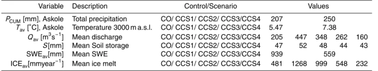
Also, in Table 4 some relevant weather and hydrological variables are reported for the four investigated glaciers’ scenarios. Table 5 contains statistical flow indicators as reported.

The CCSM3 model provides for the reference period 2050–2059 increased temper-ature of₊1.9◦C on average against 2000–2009, together with increased precipitation,

5

+20% or so. Besides modified weather, the resulting projected pattern depends upon glacier coverage scenario.

When considering unchanged glacier coverage (CCS1 scenario), discharges at Shi-gar bridge in Fig. 7 is increased in practice everywhere during the ablation season, and increased consistently on average (447 m3s−1, vs. 205 m3s−1during 1985–1997).

Av-10

erage snow cover upon the catchment decreases from 559 mm to 939 mm during the control period (Table 4).

Ice melt increases to 1268 mm year−1 vs. 481 mm year−1, as a consequence of in-crease temperature at altitudes with noticeable glacier cover area. Index flood, or average of greatest annual peak floods increases from 951 m3s−1to 2213 m3s−1, due

15

to the combined action of increased temperature and precipitation during summer and fall, the latter falling more under liquid form. Also, as a side effect of increased pre-cipitation and melting average soil moistureS is slightly increased under CCS1 and less under CCS2 scenarios (52 mm vs. 47, and 48 mm vs. 47 respectively, see Ta-ble 5), thus reaching more often saturation, and aiding in fast overland flow formation,

20

according to Eq. (5).

When decreasing glaciers’ size is considered, the effect of ice melt tends to decrease (for CCS2, 999 mm year−1, for CCS3, 548 mm year−1, for CCS4, 232 mm year−1, with

−10%, −25%, and −50% glacier cover respectively). In facts, the lack of glacier cover at the lowest altitudes, where temperature increase would be more effective for

25

ablation, results into a decrease of the latter.

(23)

HESSD

8, 3743–3791, 2011

D. Bocchiola et al.

Title Page

Tables Figures

◭ ◮

Back Close

Full Screen / Esc

Discussion

P

a

per

|

Dis

cussion

P

a

per

|

Discussion

P

a

per

|

Discussio

n

P

a

per

|

Analysis of the FDCs in Fig. 8 displays for scenarios CCS1, CCS2, and CCS3 a more variable flow regime with respect to the control period. In facts, higher discharges are seen during thaw season, and lower during dry season, the latter due to higher tem-peratures, drawing more moisture under evapotranspiration. Table 5 shows that flows occurring over short duration (d <182 days) increase for scenarios CCS1, CCS2, and

5

CCS3, but instead flows over longer duration decrease. A similar behaviour is seen when considering frequency flow descriptors, Q_Max_d and Q_Min_d. Q_Max_d is generally greater for CCS1, CCS2, and CCS3 than for control run. Instead,QMind is generally

lower, except for d=274, and more evidently for the shorter durations. Concerning scenario CCS4, all the indicators are below their control values, so displaying

general-10

ized flow decrease for considerable glacier down wasting.

6 Discussion

The proposed exercise of future flow projection provide some interesting insight into the main dynamics of snow and glaciers behavior. Glaciers’ covered area in our catchment is laid for approximately 83% within altitude belts 3 and 5 (i.e. between 3470 m a.s.l. and

15

5375 m a.s.l.), and for approximately 72% within belt 4 and 5 (i.e. between 4105 m a.s.l. and 5375 m a.s.l.).

A key feature of future glaciers’ down wasting as here projected is the dynamics of snow cover within these two belts. Figure 9 illustrates simulated SWE and cumulated ice meltMi within these two belts during control period and during 2050–2059. Clearly,

20

during control period, continuous snow cover within belt 5 provides shield to the un-derlying ice, so limiting ice melt to belt 4. However, under the future scenario with unchanged glacier cover (CCS1), snow cover in belt five is no more permanent, and ice ablation starts at snow thaw. Thus, onset of ablation within belt 5, containing alone 39% of total glacier area here, provides a tremendous increase of discharge from ice

25

melt. When glaciers shrinkage is considered (here case CCS4 is shown,−50% glacier

(24)

HESSD

8, 3743–3791, 2011

D. Bocchiola et al.

Title Page

Tables Figures

◭ ◮

Back Close

Full Screen / Esc

Discussion

P

a

per

|

Dis

cussion

P

a

per

|

Discussion

P

a

per

|

Discussio

n

P

a

per

|

for CCS4, belt 5−16% for CCS4), so that weighted M_i drops as well. This in turn

decreases in stream flows.

Within altitude belt 6 (5375 m a.s.l. 6010 m a.s.l.) we found continuous snow cover (not shown for shortness), so we found in practice no ice melt, indicating that above this altitude no noticeable down wasting should occur within 2059, and the ice melt

5

contributing areas should in practice be limited below 5500 m a.s.l. or so.

From what reported here, the hypothesis of a 50% shrinkage of glaciers’ area is not fully unlikely, as lack of permanent snow cover (and thus of glacier recharge) under ongoing climate warming may impact glaciers down wasting up the an area including more than 80% of the ice here. Initially, ice ablation would provide increased

dis-10

charges. Besides the obvious positive asset of increased water availability, however, increased in stream flows and peak floods may fallout into hampered water manage-ment. As soon as glacier down wasting triggers, decreased ice ablation will affect flow discharges. Our sensitivity analysis here would indicate that an ice cover shrink-age between 25% and 50%, i.e. disappearance of ice cover between 3500 m a.s.l. and

15

4500 m a.s.l. may be critical already, with considerably decreased water resources, and worst drought spells.

Our model, explicitly developed for poorly gauged basins, suffers from some possible lacks of accuracy. The proposed melt factor approach is considerably simple in view of the complex dynamics of snow and ice melts, including debris cover. Energy based

20

model are nowadays available for snow and ice melt (Lehning et al., 2002; Nicholson and Benn, 2006; Brock et al., 2007; Rulli et al., 2009), but they may require more in-formation, including sub-daily solar radiation, wind velocity and air moisture, in practice unavailable here.

Degree day approach, calibrated here vs. SCA images, is simple and

computa-25

tionally fast enough to tolerate long term simulation, while reasonably capturing the observed pattern of snow and ice melt and water fluxes.

(25)

HESSD

8, 3743–3791, 2011

D. Bocchiola et al.

Title Page

Tables Figures

◭ ◮

Back Close

Full Screen / Esc

Discussion

P

a

per

|

Dis

cussion

P

a

per

|

Discussion

P

a

per

|

Discussio

n

P

a

per

|

data are required, including local observations of air temperature and precipitation (rainfall₊snowfall), or at least some extrapolation to high altitudes. Here, for hydro-logical model calibration, we had to rely upon disaggregation of monthly data, which may introduce further noise.

One should may carry out (at least) one comprehensive survey of snow depth

distri-5

bution upon the glaciers at the onset of snow depletion, in order to link this information to the data from the lower measured stations in the basin, if available, or to initialize the model (see Bocchiola et al., 2010). Indeed, under the umbrella of the SHARE-Paprika project, we plan to carry out at least one such survey within the expected accumulation area of the Baltoro glacier (above 5500 m a.s.l. or so), which should aid in (i) setting up

10

initial SWE conditions for long term snow melt simulations, and (ii) evaluating properly melt factor DDs. However, here use of remotely sensed images, widely spread and easily available nowadays, is shown to provide considerable gain in term of snow melt modeling.

The use of extrapolated (via lapse rate) rather than measured temperatures and

pre-15

cipitation (the latter considerably uncertain) may affect the performance of the model, especially during the onset (May, June) and end (September) of the melt season, seen as critical periods here.

A most compelling issue is the assessment of soil retemption, here quantified ac-cording to the SCS-CN method. In poorly gauged watersheds as here, were soil cover

20

information may lack, bad estimation of soil abstraction may indeed mislead flood pre-diction, especially in the lowest, possibly vegetated, areas. Because soil use changes may interact with climate to modify flow occurrence in the near future, understanding of soil response is warranted henceforth.

Therefore, specific focus should be directed on estimation of soil conditions, e.g.

25

(26)

HESSD

8, 3743–3791, 2011

D. Bocchiola et al.

Title Page

Tables Figures

◭ ◮

Back Close

Full Screen / Esc

Discussion

P

a

per

|

Dis

cussion

P

a

per

|

Discussion

P

a

per

|

Discussio

n

P

a

per

|

The projected hydrological scenarios are clearly sensitive to the climate inputs. Within the present literature some works are available concerning recent and prospec-tive climate and hydrology trends within Karakoram region. Archer and Fowler (2004), and Fowler and Archer (2005) investigated Trends of temperature and precipitation dur-ing 1961–2000 for some stations in Northern Pakistan, close to our catchments here.

5

They found spatially varying results, but they highlighted a general increase of Win-ter temperature (roughly+0.6◦C in the considered period), and a cooling in summer (roughly−1◦C), together with an increase in precipitaton during Winter, Summer, and

yearly (roughly+30% on average).

Hewitt (2005), highlighted evidence of glacier expansion in the central Karakoram in

10

the late 1990s, occurring almost exclusively in glacier basins from the highest parts of the range. Possible explanations for this involve increases in precipitation in val-ley climate stations during the last four decades or so, and small declines in summer temperatures, which may indicate positive trends in glacier mass balance. Here, our reference CCSM3 model provides during Summer (JAS) an increase of 2.3◦C on

av-15

erage in the area (2000–2009 vs. 2050–2059), as an increase in precipitation in the order of 21% or so during Winter (JFM).

As reported in the introduction Akhtar et al. (2008) used SRES A2 scenario (2071– 2100) by the PRECIS Regional Climate Model and HBV hydrological model to simulate future (2071–2100) discharge in three catchments in the HKH, and found increased

dis-20

charge for 100% and 50% glacier scenarios, and predicted in stead a drastic decrease in the 0% scenario. Their change in temperature (from 1961–2000) is of +4.5-4.8

◦

C yearly (+4.7–4.8◦C in Winter, +4.2–4.8◦C Summer), against our +1.9◦C yearly (₊1.8◦C Winter ,₊2.3◦C in Summer, 2050–2059 vs. 2000–2009), which projected to 2100 would be roughly +3.9◦C yearly (1961–2000 vs. 2071–2100, +4.8◦C in

Sum-25

(27)

HESSD

8, 3743–3791, 2011

D. Bocchiola et al.

Title Page

Tables Figures

◭ ◮

Back Close

Full Screen / Esc

Discussion

P

a

per

|

Dis

cussion

P

a

per

|

Discussion

P

a

per

|

Discussio

n

P

a

per

|

Their results concerning increasing discharge for 50% glacier cover do indicate dif-ferent results with respect to our findings here. However, this may either be due to the their highest temperature, providing more melting upon a smaller area, or to a different way of calculation of glacier cover (e.g. without considering altitude distribution as we did here?). Eventually, we may state that our results here broadly speaking agree with

5

their findings.

Notice here that, albeit we used SCA from MODIS for ice melt validation, our hydro-logical model does not require use of SCA for hydrohydro-logical simulation (like e.g. SRM model, Rango, 1992; Immerzeel et al., 2010), as it implicitly accounts for snow cover budget (and depletion). The same applies in principle to ice cover. This means that, in

10

case an initial condition concerning ice cover area and ice thickness (i.e. volume) would be available within each altitude belt (and neglecting or modeling in some way ice flow down slope), ice budget could be explicitly tracked within the catchment. Therefore, future work may be devoted to estimating in some way ice volume, in order to assess full mass budget for the area (e.g. Kuhn, 2003), and climate change effect therein.

15

The approach we proposed here seems simple enough that portability to catchments nearby should be reasonably practicable. With the caveats underlined above, temper-ature and precipitation may be drawn from the low altitude network (and satellite data for reference, as we did with TRMM here). Degree day for snow and ice may be eval-uated based upon (at least) one field campaign, or taken from others studies like ours,

20

and perhaps validated with aid of satellite data for SCA. Analysis of geology and land cover maps should aid in estimating soil retemption, especially for the lowest areas. Eventually, sensitivity of hydrological cycle to climate change may be tested using re-gional models plus downscaling based upon the available ground stations as here, and benchmarked against other similar studies for consistency.

(28)

HESSD

8, 3743–3791, 2011

D. Bocchiola et al.

Title Page

Tables Figures

◭ ◮

Back Close

Full Screen / Esc

Discussion

P

a

per

|

Dis

cussion

P

a

per

|

Discussion

P

a

per

|

Discussio

n

P

a

per

|

7 Conclusions

We investigated future ablation flows from a poorly gauged glacierized watershed within HKH mountain, studied here for the first time in our knowledge. We gathered information from inhomogeneous available meteorological and hydrological data, we used data from former field campaigns to evaluate ice ablation, and we then coupled

5

glaciological concepts to hydrological modeling theory, to obtain a reasonable synthe-sis of the hydrological patterns from this glacierized area. We used remotely sensed SCA to tune a degree day approach within an area lacking of snow cover data, with interesting results.

We then projected hydrological cycle fifty years ahead from now, and we highlighted

10

the possible consequences of a warming and wetting climate, as expected according to the present literature, upon water resources down slope.

The present paper provides a relevant and possibly valuable contribution to the on-going discussion concerning flood prediction and future projections in ungauged and poorly gauged basins, and specifically to the PUB decade initiative of IAHS. The

pro-15

posed approach profits of sparse data from several sources, and is simple enough that portability to other catchments nearby should be reasonably feasible, as required for regional investigation of this high altitude, inaccessible, and yet tremendously impor-tant area. Because ungauged watersheds, and particularly high altitude glacierized ones within HKH, are thethird poleof the world, storing a tremendous amount or water

20

to be delivered to populations downstream, their duly investigation here forward seems utmost warranted.

Acknowledgements. The present work was carried out in fulfillment of the SHARE-Paprika project, funded by the EVK2CNR committee of Italy, aiming at evaluating the impact of climate change upon hydrology of the upper Indus river. We hereby acknowledge EVK2CNR committee 25