Current status of the ability of the GEMS/MACC models to reproduce the tropospheric CO vertical distribution as measured by MOZAIC

(1)

GMDD

3, 391–449, 2010

Validation of MACC models

N. Elguindi et al.

Title Page

Abstract Introduction

Conclusions References

Tables Figures

◭ ◮

Back Close

Full Screen / Esc

Printer-friendly Version

Interactive Discussion

Geosci. Model Dev. Discuss., 3, 391–449, 2010 www.geosci-model-dev-discuss.net/3/391/2010/ © Author(s) 2010. This work is distributed under the Creative Commons Attribution 3.0 License.

Geoscientific Model Development Discussions

This discussion paper is/has been under review for the journal Geoscientific Model Development (GMD). Please refer to the corresponding final paper in GMD if available.

Current status of the ability of the

GEMS/MACC models to reproduce the

tropospheric CO vertical distribution as

measured by MOZAIC

N. Elguindi1,2, C. Ord ´o ˜nez1,2,3, V. Thouret1,2, J. Flemming4, O. Stein5, V. Huijnen6, P. Moinat7, A. Inness4, V.-H. Peuch7, A. Stohl8, S. Turquety9, J.-P. Cammas1,2, and M. Schultz5

1

Universit ´e de Toulouse, UPS, LA (Laboratoire d’A ´erologie), 14 avenue Edouard Belin, Toulouse, France

2

CNRS, LA (Laboratoire d’A ´erologie), UMR 5560, 31400 Toulouse, France

3

Met Office, Atmospheric Dispersion Group, Exeter, UK

4

European Centre for Medium-Range Weather Forecasts (ECMWF), Reading, UK

5

(2)

GMDD

3, 391–449, 2010

N. Elguindi et al.

Title Page

Tables Figures

◭ ◮

Back Close

Full Screen / Esc

6

Royal Netherlands Meteorological Institute (KNMI), De Bilt, The Netherlands

7

M ét éo France, Centre National de Recherches M ét éorologiques, Toulouse, France

8

Norwegian Institute for Air Research, Kjeller, Norway

9

Laboratoire de M ´et ´eorologie Dynamique/IPSL, UPMC Univ. Paris 06, Paris, France

Received: 3 March 2010 – Accepted: 19 March 2010 – Published: 8 April 2010 Correspondence to: N. Elguindi (soln@aero.obs-mis.fr)

(3)

GMDD

3, 391–449, 2010

N. Elguindi et al.

Title Page

Tables Figures

◭ ◮

Back Close

Full Screen / Esc

Abstract

Vertical profiles of CO taken from the MOZAIC aircraft database are used to present (1) a global analysis of CO seasonal averages and interannual variability for the years 2002–2007 and (2) a global validation of CO estimates produced by the MACC models for 2004, including an assessment of their ability to transport pollutants originating

5

from the Alaskan/Canadian wildfires. Seasonal averages and interannual variability from several MOZAIC sites representing different regions of the world show that CO concentrations are highest and most variable during the winter season. The inter-regional variability is significant with concentrations increasing eastward from Europe to Japan. The impact of the intense boreal fires, particularly in Russia, during the fall

10

of 2002 on the Northern Hemisphere CO concentrations throughout the troposphere is well represented by the MOZAIC data.

A global validation of the GEMS/MACC GRG models which include three stand-alone CTMs (MOZART, MOCAGE and TM5) and the coupled ECMWF Integrated Fore-casting System (IFS)/MOZART model with and without MOPITT CO data assimilation

15

show that the models have a tendency to underestimate CO. The models perform best in Europe and the US where biases range from 0 to –25% in the free troposphere and from 0 to –50% in the surface and boundary layers (BL). The biases are largest in the winter and during the daytime when emissions are highest, indicating that current inventories are too low. Data assimilation is shown to reduce biases by up to 25%

20

(4)

GMDD

3, 391–449, 2010

N. Elguindi et al.

Title Page

Tables Figures

◭ ◮

Back Close

Full Screen / Esc

1 Introduction

Carbon monoxide (CO) is a key trace gas in the atmosphere and plays an important role in the chemistry of the troposphere by exerting a strong influence on the concen-trations of oxidants such as the hydroxyl radical (OH) and ozone (O₃) (Wotawa et al., 2001). Changes in oxidation by OH due to changes in CO concentrations could perturb

5

the concentration of greenhouse gases such as methane (CH4) and O3 (Thompson

and Ciccerone, 1986), and thus play a role in our understanding and assessment of potential climate change.

The main sources of CO are fossil fuel and biomass burning. While most biomass burning occurs in the tropics, recent studies have shown that boreal forest fires might

10

account for as much as 25% of the global CO emissions from all wildfires during anomalous boreal fire years (Goode et al., 2000; Lavou ´e et al., 2000). Gases and aerosols emitted from large wildfires can be transported thousands of kilometers downwind. In addition, due to the strong convection enhanced by forest fire activity, emissions can be injected into the upper troposphere and lower stratosphere (Jost

15

et al., 2004; Ned ´el ´ec et al., 2005; Damoah et al., 2006; Cammas et al., 2009) where the residence time is long, thus having lasting effects on radiation and stratospheric chemisty. During the summer of 2004 large wildfires burned in Alaska and Canada. Trace gases and aerosols emitted by these fires were transported as far away as Europe. A large amount of data was collected during this period as part of the

In-20

ternational Consortium for Atmospheric Research on Transport and Transformation (ICARTT) program. The ICARTT program was a massive experimental campaign co-ordinated by an international team of scientists which utilized nine aircraft, one re-search vessel, several ground-based sites in North America and the Azores, a network of aerosol-ozone lidars in Europe, satellites, balloon borne sondes, and routine

com-25

(5)

GMDD

3, 391–449, 2010

N. Elguindi et al.

Title Page

Tables Figures

◭ ◮

Back Close

Full Screen / Esc

convection parameterizations (Stohl et al., 2005). Output from these simulations pro-vide an important resource to interpret transport processes during the period of interest (see http://www.esrl.noaa.gov/csd/ICARTT/analysis/). As a result of the ICARTT effort, many studies have since provided valuable information on the effects of the gases and aerosols emitted into the atmosphere from the Alaskan/Canadian wildfires (Fehsenfeld

5

et al., 2006; Pfister et al., 2006, 2008; Bousserez et al., 2007; Real et al., 2007; Stohl et al., 2006; Damoah et al., 2006; Cammas et al., 2009; Warneke et al., 2006; Turquety et al., 2007).

Numerous studies have used chemistry transport models (CTMs) to simulate CO (Shindell et al., 2006; Kanakidou et al., 1999; Prather et al., 2001). In a study

evaluat-10

ing the ability of 26 state-of-the-art CTMs to simulate global present-day CO, Shindell et al. (2006) found that most models significantly under-estimate CO in the extrat-ropical Northern Hemisphere. Results from the study also show that the variability among models is large, which the authors claim to be due to intermodel di_fferences in representations and emissions of nonmethane volatile organic compounds (NMVOCs)

15

and in hydrologic cycles, which affect OH and soluble hydrocarbon intermediates. Un-certainties in emissions inventories are a well known problem among the modelling community. Inverse studies which attempt to disaggregate surface CO measurements into various source categories generally find much larger emissions than what is re-ported in present inventories which are calculated using a bottom-up approach. Data

20

assimilation can correct deficiencies in emission inventories and model transport thus improving model forecasts.

There have also been many modelling studies that have focused on the summer 2004 Alaskan/Canadian wildfires. Some of these studies have found that the long-range transport of fire emissions is better simulated when a high injection height is

25

(6)

GMDD

3, 391–449, 2010

N. Elguindi et al.

Title Page

Tables Figures

◭ ◮

Back Close

Full Screen / Esc

GEOS-Chem CTM, Turquety et al. (2007) found good results when a portion of the emissions was injected into the upper troposphere. Moreover, problems in available fire emission inventories have been identified. Studies have shown that current esti-mates of carbon emissions from biomass burning are not well constrained due to in-complete input data sets (French et al., 2004; van der Werf et al., 2006; Turquety et al.,

5

2007). A sensitivity analysis by French et al. (2004) indicates that ground-layer fraction consumed is the most uncertain parameter in constructing fire emission inventories. Recently, Turquety et al. (2007) constructed a daily bottom-up fire emissions inventory for North America in 2004 which takes into account the burning of the ground-layer organic matter stored in the soils, notably peat, which is quite important in boreal

re-10

gions. They estimate a total of 30 Tg CO was emitted from the Alaskan and Canadian wildfires during the summer of 2004, of which 37% (11 Tg) was due to peat burning.

One of the main objectives of the GRG (Global Reactive Gases) subproject of the EU project GEMS (Global and regional Earth-system (Atmosphere) Monitoring using Satellite and in-situ data) was to set up an operational data assimilation system for

15

chemically reactive gases on a global scale providing products to end-users on a day-by-day basis (Hollingsworth et al., 2008). Within this framework, the ECMWFs (Euro-pean Centre for Medium-range Weather Forecast) Integrated Forecast System (IFS) model was coupled to three chemistry transport models: MOCAGE (Josse et al., 2004; Bousserez et al., 2007), MOZART-3 (Horowitz et al., 2003; Kinnison et al., 2007), and

20

TM5 (Krol et al., 2005). One of the final goals of the GRG subproject was to assess the robustness of the satellite data assimilation procedures and the predictions, and to provide specific suggestions for improvement of the system.

Our first objective in this study is to present a global evaluation of the GEMS-GRG models, and more specifically to evaluate how well 4D-VAR data assimilation improves

25

(7)

GMDD

3, 391–449, 2010

N. Elguindi et al.

Title Page

Tables Figures

◭ ◮

Back Close

Full Screen / Esc

and assess the potential gain brought by the combination of on-line transport and 4D-VAR chemical satellite data assimilation. CO model outputs are compared to profiles of CO observations taken on-board commercial aircraft as part of the MOZAIC (Mea-surements of ozone and water vapor by Airbus inservice aircraft) program (Marenco et al., 1998). We focus on the year 2004 not only because this is one of the years in

5

which the GEMS-GRG simulations are available, but also because it provides a unique opportunity to evaluate the GEMS-GRG models’ ability to be used in process studies, namely the long-range transport of biomass fire plumes.

Our second objective in this study is to assess the ability of the GEMS-GRG mod-els to simulate and transport CO originating from the 2004 Alaskan/Canadian wildfires

10

and to further assess the satellite data assimilation procedures used in the GEMS-GRG subproject. Again, we have the unique opportunity of comparing results from three different CTMs forced with the same meteorology and are therefore able to infer weaknesses in the model physics or parameterizations (i.e. convective schemes and injection height parameterizations). Comparing the coupled IFS model runs with and

15

without data assimilation allows us to clearly ascertain how much the coupling can im-prove the CTMs’ performance as well as to assess to what extent data assimilation can compensate for deficiencies in fire emissions inventories. To this end, we per-form several case studies in which a CO plume originating from the Alaskan/Canadian wildfires was transported downwind as far as to the eastern United States and across

20

the Atlantic Ocean to Europe. Profiles of MOZAIC CO observations at several down-wind locations are compared to model outputs. In order to attribute emission sources to the MOZAIC observations we utilize the backward FLEXPART model simulations performed by Stohl et al. (2005). Furthermore, sensitivity tests are performed using tracers to evaluate ways in which to improve the long-range transport in the models. In

25

(8)

GMDD

3, 391–449, 2010

N. Elguindi et al.

Title Page

Tables Figures

◭ ◮

Back Close

Full Screen / Esc

addition, to test the models sensitivity to injection height several tracers are injected at various model levels.

There is considerable interannual variability in global tropospheric CO largely due to variability in boreal forest fires, therefore we begin our study by presenting mean seasonal vertical profiles of the MOZAIC CO data averaged over the period 2002–

5

2007, as well as profiles for the individual years, from several locations around the world. This allows us for the first time to present a climatology of the MOZAIC CO profile data, as well as to characterize the year 2004 which is the focus of the rest of this study.

Our first objective in this study is to present a global validation of the GEMS-GRG

10

models using MOZAIC vertical profiles of CO for the year 2004. Specifically to evaluate how well 4D-VAR data assimilation improves the simulation of CO. Our second objec-tive is to assess the ability of the GEMS-GRG models to simulate and transport CO originating from the 2004 Alaskan/Canadian wildfires and to further assess the satellite data assimilation procedures used in the GEMS-GRG subproject. This also allows us

15

to assess to what extent data assimilation can compensate for deficiencies in fire emis-sions inventories. Backward FLEXPART model simulations performed by Stohl et al. (2005) are used to attribute emission sources to the observations. Furthermore, sensi-tivity tests involving fire emission inventories and injection height are performed using tracers to evaluate ways in which to improve the long-range transport in the models.

20

Because there is considerable interannual variability in global tropospheric CO largely due to variability in boreal forest fires, we begin our study by presenting mean seasonal vertical profiles of the MOZAIC CO data averaged over the period 2002–2007, as well as profiles for the individual years, from several locations around the world. This allows us for the first time to present a climatology of the MOZAIC CO profile data, as well as

25

(9)

GMDD

3, 391–449, 2010

N. Elguindi et al.

Title Page

Tables Figures

◭ ◮

Back Close

Full Screen / Esc

2 Data and model descriptions 2.1 Measurement data

CO measurements taken as part of the European funded MOZAIC programme (Mea-surements of ozone and water vapour by Airbus inservice aircraft) are used for model validation in this study. The MOZAIC programme, initiated in 1993, is designed to

col-5

lect O₃, CO and water vapour data, using automatic equipment installed on-board several European long-range passenger airliners flying regularly all over the world (Marenco et al., 1998). The main objective of the MOZAIC programme is to build a comprehensive dataset of in-situ observations of these trace gases in the upper troposphere (UT) and lower stratosphere (LS) and in vertical profiles. The MOZAIC

10

dataset (1994–2009) is being intensively used for studies of the composition of the at-mosphere, trend assessments, chemical and dynamical analyses, validation of CTMs and of satellite retrievals, as well as to evaluate the impact of the global aircraft fleet on the atmosphere. MOZAIC data are available both at cruising altitude and during ascents and descents into the airports. CO measurements are made with an improved

15

version of a commercial model 48CTL from Thermo Environment Instruments, based on the Gas Filter Correlation principle of infrared absorption by the 4.67 micron fun-damental vibration-rotation band of CO (Nedelec et al., 2003). CO measurements are taken every 30 s and have a precision of±[5 ppbv±5%].

For this study, we use CO vertical profile MOZAIC data taken during the ascent

20

and descent of aircraft at various airports. The raw data are averaged over 150 m height intervals. The monthly statistical scores presented in this study are based on daily averaged profiles. The number of profiles per day varies between airports. For example, three aircraft equipped with MOZAIC instruments are based in Frankfurt, thus there can be as many as six profiles per day available for Frankfurt. However, only one

25

(10)

GMDD

3, 391–449, 2010

N. Elguindi et al.

Title Page

Tables Figures

◭ ◮

Back Close

Full Screen / Esc

The number of profiles per day at a given airport is also determined by factors such as instrumentation failure or the daily aircraft routing by the airlines. As a result, there may be no profiles available on some days at a given airport. The numbers of days with available profiles at each airport used in this study are indicated on each graph presented.

5

2.2 GEMS GRG model simulations

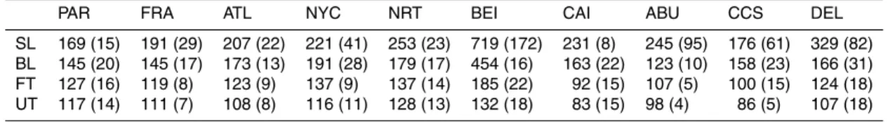
The IFS model is a state-of-the-art numerical weather prediction model with 4D var data assimilation capacities (Inness et al., 2009). In this study we analyse two simulations performed with the IFS model coupled to the chemistry transport model MOZART-V1 for the year 2004 (details of the coupling can be found in Flemming et al., 2009). The

10

first is a control run which uses no data assimilation at all, and is hereafter referred to as CTRL. The second simulation uses the full data assimilation (including total col-umn CO MOPITT data) and is hereafter referred to as ASSIM. In addition, we anal-yse simulations from the three stand-alone GEMS-GRG CTMs (MOZART-V10 (MOZ), TM5-V10:version KNMI-cy3-GEMS (TM5) and MOCAGE (MOC)). A brief description

15

of all models is given in Table 1. The set-up for the ASSIM model is identical to the CTRL model except for the addition of data assimilation (Inness et al., 2009). Further details can be found in Flemming et al. (2009). Note that the stand-alone version of MOZART is a later version than that which was coupled to the IFS model. The main upgrades are that the RETRO ship emissions have been replaced by estimates based

20

on Corbett and Koehler (2003) and the East Asian anthropogenic emissions have been replaced by the REAS inventory (Ohara et al., 2007) but keeping the original RETRO seasonality. In addition, several chemical reaction rates have been updated to JPL-06 (Sander et al., 2006).

To perform the tracer transport simulations used for the sensitivity tests, we use the

25

(11)

GMDD

3, 391–449, 2010

N. Elguindi et al.

Title Page

Tables Figures

◭ ◮

Back Close

Full Screen / Esc

the CTRL and ASSIM simulations. For the injection height sensitivity test, tracers are injected at the surface, 6 and 8 km and the Turquety emissions inventory is used.

2.3 FLEXPART model simulations

In order to attribute emission sources to the MOZAIC observations we utilize the back-ward model simulations for the summer 2004 performed by the FLEXPART Lagrangian

5

particle dispersion model (Stohl et al., 2005) at NOAA as part of the ICARTT pro-gram. For the simulations used in this analysis, the FLEXPART model was driven by model-level data from ECMWF. The data from the 60 model levels were retrieved fully mass-consistently from ECMWF data in a spectral resolution of T511. The derived gridded data has 1×1 degree resolution globally, but a 0.36×0.36 degree nest is used

10

in the region 108 W–18 E and 18 N–72 N. For emission input, the emission inventory of the EDGAR information system (version 3.2, Olivier and Berdowski (2001)) on a 1×1 degree grid is used outside North America. Over most of North America, the

inventory of Frost et al. (2006) is used. This inventory has a resolution of 4 km and also includes a list of point sources. Previous experience has shown that Asian

emis-15

sions of CO are underestimated (probably by as much as a factor of 2 or more) in the EDGAR inventory, while American CO emissions maybe overestimated. For wild-fire emissions of CO, the model uses a daily inventory which was compiled from daily burn areas provided by the Center for International Disaster Information and MODIS hot spot data (further details can be found at http://www.esrl.noaa.gov/csd/ICARTT/

20

analysis/DAILY FIRE EMISSIONS). Several simulations are performed using various injection heights in which the fire emissions are evenly distributed from the surface up to a certail model level (150 m, 1 km, 3 km, and 10 km).

2.4 Evaluation statistics

Since a large part of the GEMS project was devoted to model validation, much

con-25

(12)

GMDD

3, 391–449, 2010

N. Elguindi et al.

Title Page

Tables Figures

◭ ◮

Back Close

Full Screen / Esc

The atmospheric species concentrations can vary by orders of magnitude, thus an im-portant criterion of the metrics was the use of relative (normalized) definitions. In bias assessment when the mean observation is used as the reference, there is an asym-metry between cases of under- and over-prediction. In order to avoid this asymasym-metry, the modified normalized mean bias (MNMB), which is a normalization based on the

5

mean of the observed and forecast value, has been adopted as the most appropriate definition of bias within the GEMS/MACC project and is used in this study. The MNMB is calculated as follows,

MNMB= 2

N X

i

_f

i−oi

f_i₊o_i

·100% (1)

wheref_i and o_i represent the model forecast and observed values, respectively. The

10

MNMB is bounded by the values –200% and+200%.

3 MOZAIC CO profiles

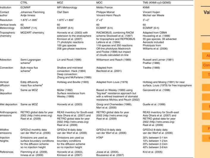
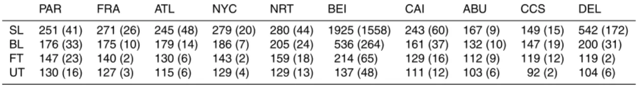
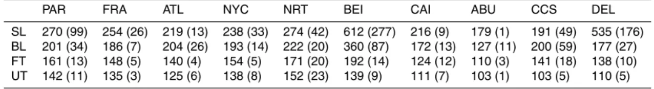
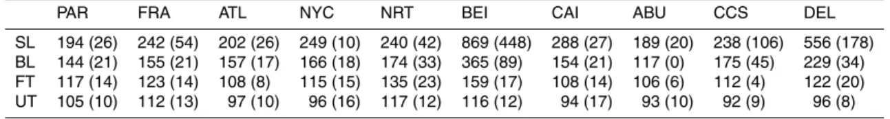
We begin this study by presenting the characteristics of seasonal vertical profiles of MOZAIC CO data averaged for the period 2002–2007 from several airports. Based on the availability of data, the following 10 airports were selected to represent different

15

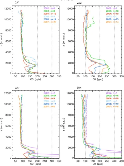
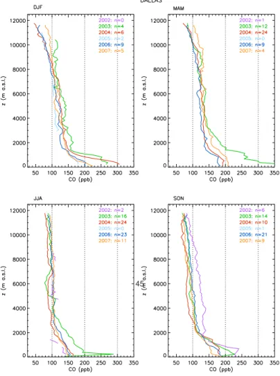
regions of the world: Frankfurt and Paris for Europe, Beijing and Tokyo for East Asia, Caracas and Delhi for low latitude regions, Atlanta and Dallas for the US, and Abu Zabi and Cairo for the Middle East. Mean seasonal CO profiles for the whole period, as well as the profiles for the individual years, are presented in Figs. 1–6 for each of the above mentioned airports. It should be noted that there is a large discrepency in the

20

number of flights (as indicated on each graph) between the various airports as well as from year to year. Therefore, not all averages for each airport and year are statistically robust.

The 2002–2007 averaged seasonal profiles presented in Fig. 1 show the seasonal and vertical characteristics of CO as well as its regional variability. In general, the

25

(13)

GMDD

3, 391–449, 2010

N. Elguindi et al.

Title Page

Tables Figures

◭ ◮

Back Close

Full Screen / Esc

2 km height with concentrations above 150 ppb and a relatively constant profile in the free troposphere with concentrations between 80 and 130 ppb. A noticeable exception is Caracas which has a layer of higher concentrations between 1 and 3 km due to its particular location in a valley 1000 m a.s.l. Globally, throughout the troposphere, CO concentrations are highest in winter and spring (DJF and MAM in the Northern

5

Hemisphere) and lowest in summer and fall (JJA and SON in the Northern Hemisphere) as determined by the seasonal variations of OH (main sink for CO).

In terms of regional variability, Beijing by far has the highest concentrations in the lower troposphere where values reach 2730 ppb near the surface during the winter. Beijing’s polluted lower troposphere is also considerably thicker than in other cities,

ex-10

tending from the ground up to about 4 km. Concentrations in Delhi are also quite high, reaching up to 997 ppb at the surface during SON. In the mid to upper troposphere, Tokyo has CO concentrations as high as those of Beijing, most probably revealing the export of continental Asian pollution. At the other extreme is Abu Zaby which has the lowest CO concentrations, at least in the lower troposphere (less than 200 ppb at the

15

surface). Globally, concentrations increase eastward from Europe to Japan.

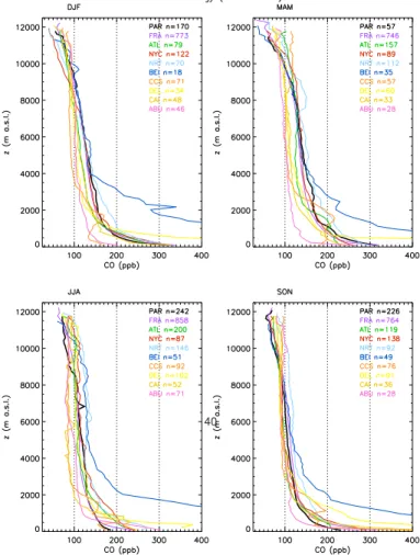
The interannual variability in the seasonal averages is shown in Figs. 2–6. Over Frankfurt (Fig. 2), there is little variability in CO during DJF compared to the JJA and SON seasons. This is mostly due to fire emissions as well as photochemical activity which is more favorable in JJA and SON. In JJA, the years 2002 and 2003 have notably

20

higher concentrations throughout the troposphere than the following years. In JJA 2003, Europe experienced a summer heat wave with anomalous concentrations of O₃ and CO over Frankfurt, especially in August (Tressol et al., 2008; Ord ´o ˜nez et al., 2010). In fall, concentrations in 2002 are considerably higher than the climatological mean. This likely reflects the hemispheric influence of the intense boreal forest fires in

25

(14)

GMDD

3, 391–449, 2010

N. Elguindi et al.

Title Page

Tables Figures

◭ ◮

Back Close

Full Screen / Esc

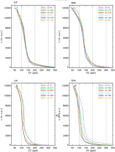
Figure 3 shows the CO profiles over Beijing, one of the most polluted cities in the world. A detailed O3 climatology can be found in Ding et al. (2008). Note that the

scale for Beijing ranges from 0–2500 ppb, unlike in the other plots where the scale ranges from 0–350 ppb. It is also worth noting that there are fewer flights available over Beijing (184) compared to Frankfurt (3801), thus the statistics are less robust. Again,

5

the highest CO concentrations near the surface occur during DJF. The year 2004 was particularly bad with surface concentrations reaching as high as 5725 ppb during DJF. During the other two years in which flights were available (2002 and 2003), CO surface concentrations range between 1000 and 1500 ppb. There is significant interannual variability during all seasons in the lower troposphere, probably due to the various and

10

intense local to regional sources but also to the small number of flights available for each year.

The CO layer in the lower troposphere over Caracas is thickest during MAM when the average concentration reaches 225 ppb near the 2 km layer (Fig. 4). The inter-annual variability is also greatest during the spring which corresponds to the regional

15

biomass burning period. Surprisingly, surface concentrations are maximum during the fall reaching 350 ppb. The year 2003 shows particularly high concentrations in both the lower troposphere and the upper troposphere during MAM. The year 2002 is also exceptional with a multi-layer CO plume below 2 km and maximum CO concentrations of more than 350 ppb during JJA and SON. As noted over Frankfurt, the period SON

20

2002 is also characterized by maximum concentrations throughout the troposphere. Although Caracas is quite far south in the tropical Northern Hemisphere, it is possible that the region was also influenced by the intense boreal fires. At this time, we are not aware of any other anomalies which could have caused such an increase in CO throughout the troposphere.

25

(15)

GMDD

3, 391–449, 2010

N. Elguindi et al.

Title Page

Tables Figures

◭ ◮

Back Close

Full Screen / Esc

year 2003 stands out as having particularly high CO concentrations in the lower tropo-sphere throughout the year (except in SON), with concentrations around one standard deviation above the climatological average. As found at other locations, very high con-centrations throughout the troposphere are present during SON 2002, reflecting the global impact of the boreal fires at this time.

5

Lastly, CO profiles over Cairo are presented in Fig. 6. The largest interannual vari-ability in the lower troposphere occurs during DJF (max in 2003). As in the other regions, SON 2002 presents high CO concentrations throughout the troposphere.

In summarizing the interannual variability of the CO profiles, Figs. 2–6 have shown that the strongest year to year differences occur in DJF and SON. There is no

system-10

atic feature in DJF and this strong variability may be due to the variability in local emis-sions and transport in the absence of destruction by OH. A strong positive CO anomaly throughout the troposphere in the Northern Hemisphere from fall 2002 through sum-mer 2003 has been linked to high levels of boreal forest fire activity, particularly in Russia, during this time (Edwards et al., 2004; Yurganov et al., 2005; Kasischke et al.,

15

2005). The MOZAIC data captures this anomaly well, particularly during the fall of 2002, giving further evidence and emphasizing the Northern Hemispheric impact of these fires. Furthermore, it is worth noting that the MOZAIC database has allowed for the characterization of the CO anomaly in terms of vertical profiles (high concentrations throughout the troposphere). Our dataset has also given a broader picture by

includ-20

ing other sites further south than those described in Yurganov et al. (2005) (Caracas for example). It is interesting that our dataset reveals that the anomaly in SON 2002 was more intense and extensive throughout the troposphere (up to 10 km) than the anomaly in summer 2003. The top-down estimates of CO emission anomalies pro-duced by Yurganov et al. (2005) are considerably larger for 2003 than 2002. However,

25

(16)

GMDD

3, 391–449, 2010

N. Elguindi et al.

Title Page

Tables Figures

◭ ◮

Back Close

Full Screen / Esc

in spring/summer 2003 is that the summer OH maximum leads to more breakdown of CO. Edwards et al. (2004) suggest that the impact of a particular emission event will depend on when it occurs in relation to the OH annual cycle. In a sensitivity test, they found that CO from fires which occur in late summer/early fall rather than early summer will persist longer in the atmosphere and have a more significant impact.

5

Finally, despite the Alaskan/Canadian wildfires that occured during the summer, globally the year 2004 had comparably lower CO concentrations. As we have selected this year to evaluate the models performance, it is an important point to keep in mind. Seasonal mean concentrations and standard deviations over the selected airports are given in Tables 2–5. These tables provide not only a quantitative reference for the

10

global evaluation presented in the next section, but also an available reference for the wider community (modelling, satellite, regional air quality, etc.) for validation purposes.

4 Global assessment of modelled CO with MOZAIC data

In this section we compare modelled estimates of monthly averaged CO from the stand-alone CTMs (MOZ, TM5 and MOC) and the coupled IFS/MOZART-V1 system

15

to the observed MOZAIC CO data measured near several airports during the year 2004. As a sensitivity test of the data assimilation process, we analyze both a coupled IFS/MOZART-V1 simulation with full data assimilation (ASSIM) and a control run with no data assimilation (CTRL). Because we are most interested in assessing how the assimilation of CO satellite data affects the simulation, ideally our control simulation

20

would exclude only the assimilation of CO. However, because of limited computer re-sources the control simulation did not assimilate meteorological observations itself but was updated to meteorological fields from ECMWF operational analysis every 24 h. This implies small differences in the underlying wind fields but as shown in Flemming et al. (2009), these meteorological differences do not noticeably change the forecast

25

(17)

GMDD

3, 391–449, 2010

N. Elguindi et al.

Title Page

Tables Figures

◭ ◮

Back Close

Full Screen / Esc

It should also be noted that the MOC CTM was only run for the months of January– September. The models are being compared with the profile data over the 10 airports representing the different regions of the world presented in the previous section. An im-portant point to keep in mind while interpreting the results is that we are are comparing point data over cities to model grid boxes, thus we might expect some underestimation

5

by the models particularly near the surface.

The modified normalized mean biases (MNMB) for CO are calculated at different atmospheric layers for each month using daily averaged profiles from the various airports (Figs. 7–11). The different atmospheric layers are defined as follows: sur-face layer (<950 hPa), boundary layer (950–850 hPa), free troposphere (850 hPa up

10

to 1 km below the tropopause) and upper troposphere (1 km below the tropopause up to the tropopause, where the tropopause is defined as the highest level with a lapse rate lower than 2 K/km). In order to conserve space, figures are shown for only one of the airports from each of the five regions of interest, however we ana-lyze and discuss results from all ten airports. Figures for the remaining five airports are

15

provided as supplementary material (http://www.geosci-model-dev-discuss.net/3/391/ 2010/gmdd-3-391-2010-supplement.pdf).

In Europe (Frankfurt and Paris), the models generally underestimate CO except in the upper troposphere where they tend to overestimate it (Fig. 7). Overall, the cou-pled IFS/MOZART-V1 model has significantly smaller biases than the three stand-alone

20

CTMs. In most cases, the CTRL biases are smaller than the CTM biases but not as small as the ASSIM biases, suggesting improvements made by the coupled model are likely the result of both the CO assimilation as well as the better transport provided by the IFS coupled dynamical model. However, it is difficult to make conclusive state-ments about the performance of the CTRL model since it was only run for June and

25

(18)

GMDD

3, 391–449, 2010

N. Elguindi et al.

Title Page

Tables Figures

◭ ◮

Back Close

Full Screen / Esc

during the fall months when concentrations are minimum. This further supports the argument that a significant part of the model biases are related to deficiencies in the emission inventories which are too low. Among the CTMs, MOC has the highest biases during the summer months, but performs much better during the first part of the year (January–April). Biases in the upper troposphere are mainly between±25%. Unlike in

5

the free troposphere, improvements made by the ASSIM model are much less evident in the upper troposphere where the MOPITT signal is very weak.

Compared to Europe, negative biases are much higher in East Asia (Tokyo and Beijing), reaching>100% near the surface during some months over Beijing (Fig. 8). Similar to Europe, CO is mostly underestimated in the free troposphere, boundary

10

and surface layers. Biases are especially high over Beijing near the surface and in the boundary layer where even the coupled models are not performing well. In fact, in the boundary layer the CTMs have lower biases than the coupled models during most of the year. This is most likely due to the fact that both MOZ and TM5 use the REAS inventory which has higher emissions over South-east Asia than the RETRO

15

inventory used by the coupled models. In the free troposphere, the ASSIM model does show improvement compared to the CTMs during most months. Although biases are slightly smaller over Tokyo (not shown), they are still quite large with values>50% near the surface during much of the year. Unlike over Beijing, the ASSIM model shows improvement over the CTMs in many of the cases in the surface and boundary layers,

20

although not in all months. Perhaps this is because the assimilation is able to capture much of the pollution originating upwind in Northern China. MOC performs quite well in the lower troposphere over Tokyo compared to the other CTMs.

Biases in the low latitude regions which are represented by Delhi in Southeast Asia Fig. 9 and Caracas in tropical South America (not shown) are less consistent than in

25

(19)

GMDD

3, 391–449, 2010

N. Elguindi et al.

Title Page

Tables Figures

◭ ◮

Back Close

Full Screen / Esc

where CO concentrations can be very high near the surface, it is not clear whether there is an improvement with the coupled models, especially in the surface and bound-ary layers. Likewise over Caracas, we do not see a clear improvement in the biases of the coupled models as compared to the stand-alone CTMs.

Biases over the US (Atlanta and Dallas) indicate that the models generally

under-5

estimate CO in the free troposphere and surface and boundary layers, as found over most of the other cities (Fig. 10). CTM biases are mostly between –25 and –50% near the surface and between 0 and –25% in the free troposphere, over both Atlanta and Dallas. In this region, there is a clear improvement in the biases of the ASSIM model as compared to the CTMs, especially during the late winter and early spring months

10

as also noted over Europe. This is perhaps due to the fact that the assimilation is com-pensating for biases in the emissions which are larger during this time of year when CO concentrations are maximum, and also due to the better performance by the coupled model during the transitional spring season in the mid-latitude regions. In the free tro-posphere, biases are mostly between 0 and –25%, and the CTMs perform best during

15

the late summer and early fall months.

Biases for the Middle East region are represented by Abu Zaby (Fig. 11) and Cairo (not shown). During the summer, biases are high (and negative) near the surface over Abu Zaby (>50%), but of smaller magnitude during the rest of the year when data are available. In the boundary layer, the CTMs tend to underestimate CO by

20

0–35%, while the ASSIM model has a tendency to overestimate with biases ranging from –5 to+15%. The ASSIM model also tends to slightly overestimate CO in the free troposphere, which is a feature generally not observed over most of the other cities. Unfortunately, there are not many flights over Cairo to compare results. However, during the few months in which data are available (January, February, March, May and

25

October) the ASSIM model biases are smaller than for the CTMs most of the time, particularly in the boundary layer and free troposphere.

(20)

GMDD

3, 391–449, 2010

N. Elguindi et al.

Title Page

Tables Figures

◭ ◮

Back Close

Full Screen / Esc

hours to determine whether the time of day has an effect on the biases. In general, biases tend to be lower during the nighttime than at daytime in the surface (by 0–25%) and boundary (by 0–15%) layers, while in the free troposphere there is little difference. Because diurnal changes are not represented in the emissions data, this indicates that the emissions are actually represented by their minimum within a daily cycle.

5

In order to assess how well the models reproduce the day-to-day variability in Eu-rope and the US, two examples of daily averaged CO timeseries are presented in Figs. 12–13. Overall, the IFS coupled system with assimilation, ASSIM, is adequately reproducing both the variability and concentrations. However, there are some peaks that the IFS coupled system is not able to reproduce, such as on 22 July at 500 hPa

10

over Frankfurt, which might occur for several reasons. It generally takes the MOPITT satellite about 4 days to get full coverage of the Earth, thus specific events such as this may not be captured by MOPITT. Another possible reason is that meso-scale CO plumes may not be seen by MOPITT, so are therefore not assimilated. In general, the CTRL simulation does not capture the daily variability in CO as well as the ASSIM

15

simulation. This is especially evident over Frankfurt where CO peaks during the latter half of July are reproduced by the ASSIM simulation but not the CTRL simulation. This is clear indication of the improvements gained by the assimilation process. The free CTMs underestimate CO concentrations, particularly at lower levels (850 and 700 hPa). CTM biases are of smaller magnitude at the upper levels (500 and 300 hPa). In general

20

at the lower levels, MOCAGE tends to have the largest biases while MOZART and TM5 perform noticeably better, especially over Frankfurt. For example, over Frankfurt in July at 850 hPa MOCAGE has a MNMB of –33%, while MOZART and TM5 have MNMBs of –13 and –16%, respectively. Over Atlanta at 850 hPa in June MOCAGE has a MNMB of –29%, while MOZART and TM5 have biases of –18 and –21%, respectively. In

gen-25

(21)

GMDD

3, 391–449, 2010

N. Elguindi et al.

Title Page

Tables Figures

◭ ◮

Back Close

Full Screen / Esc

5 Biomass burning signature in MOZAIC data

In this section we examine how well the stand-alone CTMs and the IFS coupled sys-tem with assimilation (ASSIM) can simulate the long-range transport of CO plumes originating from biomass burning during the 2004 Alaskan/Canadian wildfires at three downwind locations: Washington, Paris and Frankfurt. As in the previous section,

5

we include the coupled IFS/MOZART-V1 control simulation with no data assimilation (CTRL) in our analysis in order to provide some insight on the sensitivity to the assim-ilation process. We select four case studies, based on the availablity of FLEXPART model simulations, in which CO plumes have been transported from Alaska. First we present MOZAIC vertical profiles for each case study along with the FLEXPART

di-10

agnosis which supports the claim that the CO plumes did actually originate from the Alaskan/Canadian wildfires. Then we examine how well the stand-alone CTMs and IFS coupled system with assimilation are able to reproduce the CO plumes observed in the MOZAIC data.

In addition, following results from other studies which suggest that emissions from

15

boreal forest fires can be injected as high into the atmosphere as the upper tropo-sphere/lower stratosphere (Jost et al., 2004; Damoah et al., 2006; Leung et al., 2007), we investigate to what extent the injection height in the IFS model affects the long-range transport of fire emissions. Furthermore, to test how sensitive the model is to the fire emissions inventory, an additional simulation is performed using the inventory

20

compiled by Turquety et al. (2007) for North American during the year 2004, rather than the GFED inventory.

5.1 Description of case studies

– CASE 1: measurements were taken on a descending flight over Paris on 22 July 2004 at 03:24 UTC landing time (Fig. 14, top left). A CO plume is present in the

25

(22)

GMDD

3, 391–449, 2010

N. Elguindi et al.

Title Page

Tables Figures

◭ ◮

Back Close

Full Screen / Esc

emissions present in concentrations of 40–160 ppb at this level. There is also an-other FLEXPART plume between 8–10 km with concentrations up to 160 ppb, al-though in the MOZAIC data this plume is higher and much weaker (110 ppb). The CO plume between 3–6 km is present in the FLEXPART simulations regardless of the injection height used, therefore this case is considered rather insensitive to

5

injection height. The contribution of European emissions ranges from 0–30 ppb from 500 m to 2 km.

– CASE 2: measurements were taken on an ascending flight from the Frankfurt air-port on 22 July 2004 at 08:48 UTC takeofftime (Fig. 14, top right). A very deep CO layer exists between 4.5–7 km as well as a thin layer around 8.5 km with

con-10

centrations up to 225 ppb. The FLEXPART backward model run with an injection height of 10 km simulates a CO plume in which the altitude range is in good agree-ment with MOZAIC observations, and in this case the FLEXPART results are very sensitive to the assumed injection height. Peaks of Flexpart CO for biomass fires is of around 160 ppbv, and when added to a tropospheric background of about

15

100ppbv makes CO in excess of 220 ppbv, which is in relatively good agreement with the MOZAIC profile. European emissions significantly contribute to CO below 2 km with a magnitude of 60 ppbv.

– CASE 3: measurements were taken on an ascending flight from the Frankfurt airport on 23 July 2004 at 08:54 UTC takeo_ff time (Fig. 14, bottom left). The

20

CO plume here lies between 3.5–5 km over Frankfurt with concentrations up to 275 ppbv. The FLEXPART backward model run leads to CO concentrations of up to 120 ppb between 4–5.5 km in the upper part of the CO plume seen in the MOZAIC data. According to the FLEXPART simulations, CO concentrations are sensitive to the injection height. The contribution of European emissions below

25

4 km range from 0 to 90 ppb.

(23)

GMDD

3, 391–449, 2010

N. Elguindi et al.

Title Page

Tables Figures

◭ ◮

Back Close

Full Screen / Esc

case was also examined by Cammas et al. (2009) in a study involving the injection of biomass fire emissions into the lower stratosphere and its long-range transport. There are 3 distinct CO plumes present; the first between 2.5 and 4 km, the sec-ond between 4.0 and 6 km, the third between 6 and 8 km. The CO concentrations within the plumes are around 150–190 ppb. The FLEXPART backward model run

5

with an injection height of 10 km indicates that the CO mixing ratios observed in the Washington area originated from the Alaskan wildfires. The altitudes of the 2 layers of the North American biomass burning tracer transported by FLEXPART are well correlated with 2 of the 3 layers observed by MOZAIC. When a 10 km injection height is specified, maximum CO concentrations in the 7 km and 3.5 km

10

altitude layers are about 115 and 70 ppb, respectively. None of the CO plumes ex-ist, except for a very weak one between 3–4 km, when an injection height of 3 km, 1 km or 150 m is used, suggesting that this case is highly sensitive to injection height. CO resulting from American anthropogenic emissions are only present between 0 to 3–4 km, with concentrations from 50 ppb to 80 ppb near the surface.

15

5.2 Model comparison

The modelled and observed CO vertical profiles for each of the case studies are pre-sented in Fig. 15. In case study 1 over Paris, the only CTM which is able to capture a small hint of the CO plume is MOZ. Although the concentrations in the MOZ plume are very weak and the layer is too thick and not well placed in comparison to the MOZAIC

20

data, it is encouraging that the model is able to transport the CO emissions such long distances. One factor to keep in mind is the coarser horizontal resolution of MOC and TM5 (3◦×2◦) compared to MOZ and the coupled models (1.875◦×1.895◦) which inhibits

their ability to represent small-scale plumes. The ASSIM model does a slightly better job than the stand-alone MOZ model in terms of concentration, but the plume is still

25

(24)

Frank-GMDD

3, 391–449, 2010

N. Elguindi et al.

Title Page

Tables Figures

◭ ◮

Back Close

Full Screen / Esc

furt, only the coupled models are able to capture the CO plume. Similarly to case 1, the ASSIM model does a slightly better job than CTRL, but the plume in both models are also still very weak in comparison to the MOZAIC data. In case 3 over Frankfurt, only the ASSIM model shows signs of a CO plume, although it is even weaker than in cases 1 or 2.

5

In case 4 over Washington, the CO plume is more complex with 3 distinct layers. From the 3 CTMs only MOZ shows signs of 2 weak plumes which to some extent match the 4 km and 7 km layer plumes in the MOZAIC data. The ASSIM model also shows weak signs of the multi-layer CO plume found in the data, whereas the CTRL model does not, indicating that it is the assimilation that is improving the long-range

10

transport of CO. Unlike in cases 1–3, in the lower troposphere below about 2.5 km the ASSIM model over-estimates CO by about 50 ppb in comparison to the MOZAIC data, whereas the biases for the CTRL model are substantially smaller. It is possible that this is an e_ffect of the simplified assimilation process in the IFS coupled system in which the total column CO is assimilated without further information of it’s vertical

15

profile. Because MOPITT’s sensitivity to CO concentrations in the lower troposphere varies widely (Deeter et al., 2007), a more realistic approach to the assimilation process would be to determine from the analysis of MOPITT averaging kernels where and when the measurements offer useful sensitivity to lower tropospheric CO.

5.3 Sensitivity to fire emissions

20

In order to evaluate how sensitive the IFS/MOZART-V1 model is to the fire emis-sions inventory we perform two tracer simulations, one using the 8-daily GFEDv2 inventory and another using the daily inventory compiled by Turquety et al. (2007). The emissions from both inventories are shown in Fig. 6 in the on-line supplementary material (http://www.geosci-model-dev-discuss.net/3/391/2010/

25

(25)

GMDD

3, 391–449, 2010

N. Elguindi et al.

Title Page

Tables Figures

◭ ◮

Back Close

Full Screen / Esc

significant impact on the long-range transport of CO. Tracer profiles from the two sim-ulations as well as the corresponding MOZAIC CO profile from the four case studies discussed in the previous section along with four additional examples are presented in Fig. 16. The solid lines represent tracers injected at the surface as in the CTRL and ASSIM simulations. The dashed and dotted lines are discussed in the following

sec-5

tion regarding injection height. Although we can not directly compare the tracer plumes which only represent CO due to biomass burning to the observed profiles (black solid lines), the MOZAIC CO data serve as a proxy for the location and depth of the trans-ported plumes.

In the first two cases over Washington, neither the GFED nor the Turquety tracer

10

emitted at the surface show the presence of a significant plume. However in the rest of the cases which are over Paris and Frankfurt, the Turquety tracer plume is clearly in better agreement with the observed CO plumes than the GFED plume. One possible factor which might explain why the plumes seem better represented over Europe than Washington, which is closer to the sources, could be related to the period in which

15

the fires occurred. The two cases over Washington occurred near the end of June and the fire emissions previous to those days were weaker, while the cases over Paris and Frankfurt occurred in July when the fires were more intense (see Fig. 6 in the online supplementary material, http://www.geosci-model-dev-discuss.net/3/391/2010/ gmdd-3-391-2010-supplement.pdf). Thus, the larger amount of emissions emitted in

20

July would more likely be transported farther downwind. Another contributing factor could be related to the injection height. The meteorological conditions and the intensity of the fires during the late June fires may have been more favorable to higher injection heights (Damoah et al., 2006), and as a consequence the surface injection height used by the model was not sufficient to reproduce the observed plume. This is supported by

25

the fact that the FLEXPART simulation for case 4 (30 June over Washington) was also found to be highly sensitive to the injection height (see Fig. 14, bottom right). Note that the FLEXPART simulations also used fire emissions at daily resolution.

(26)

cur-GMDD

3, 391–449, 2010

N. Elguindi et al.

Title Page

Tables Figures

◭ ◮

Back Close

Full Screen / Esc

rent fire emission inventories for modelling purposes (French et al., 2004; van der Werf et al., 2006; Turquety et al., 2007). However, despite the clear improvement in using the Turquety data, the plumes in most of the cases are still notably weaker at the down-wind locations over Europe than the observed CO plumes, except perhaps on 22 July when the plumes are quite deep.

5

5.4 Sensitivity to injection height

For the models used in this study, emissions were injected at relatively low heights in the atmosphere (see Sect. 2 for details). We performed simulations in which a tracer is injected over the wildfire regions of Alaska/Canada during the summer of 2004 at several different model levels (surface, 6 and 8 km). The Turquety fire emissions

10

inventory is used in these simulation.

The profiles of the tracers at the various injection heights are represented by the purple lines in Fig. 16. The impact of the injection height on the long-range transport of the tracer is variable. In some of the cases, the tracers injected at 6 or 8 km produce plumes with higher concentrations than the tracer injected at the surface. For example,

15

for the two cases over Washington during late June the tracer injected at the surface does not show any presence of a plume as noted in the previous section. However, the 6 and 8 km tracers are represented by plumes over Washington, although the location and depth of the plumes do not exactly match the observed ones. In the 26 June case, both the 6 and 8 km tracer plumes are located near the same altitude as the

20

observed plume but are not as deep. In the 30 June case, the 6 km tracer plume matches quite well in location and depth to the observed lower plume but the middle and upper plumes are not represented. Contrarily, the 8 km tracer produces a multi-layered plume but it is considerably weaker than the observed one. In other cases, the injection height does not seem to have an effect on the long-range tracer transport,

25

(27)

GMDD

3, 391–449, 2010

N. Elguindi et al.

Title Page

Tables Figures

◭ ◮

Back Close

Full Screen / Esc

fire emissions occur at the same time in the same grid mesh of the model, and that convection is contributing to the vertical transport.

In order to get a broader picture of how the tracers are being transported in the model we examine spatial maps and vertical cross-sections of the different tracers on select days (Figs. 17 and 18). In comparing the spatial maps of tracer burden (integrated

5

from the surface to approxiamately 100 hPa) on 30 June, we see that although the con-centrations vary somewhat among the different tracers, the spatial pattern over North America is quite similar indicating that the surface tracer is getting transported down-wind (Fig. 17). However, the concentrations are considerably weaker than the 6 and 8 km tracer over the northeast US and Europe. The longitudinal vertical cross-sections

10

show that the largest di_fferences in tracer concentrations occur near the source region of Alaska and western Canada. This is expected since the tracers are injected at var-ious heights here, thus we see the largest concentration of the surface tracer in the lower troposphere and the largest concentration of the 8 km tracer in the mid- to upper-troposphere. Over the eastern US and Canada (50◦W to 90◦W) and Europe (0 to

15

25◦E), the 6 km and 8 km tracers have quite similar concentrations while the downwind transport is considerably weaker.

Similar maps of tracer burdens and longitudinal vertical cross-sections for 22 July are presented in Fig. 18. As in the other case, the overall spatial pattern is quite similar but the concentration varies among the tracers. The surface tracer concentrations are

20

higher near the source region and lower further downwind than the 6 and 8 km tracers. The 8 km tracer concentrations are higher than the 6 km tracer concentrations along the US Eastern seaboard but surprisingly lower in the plume extending to the northwest of Europe. Nonetheless, in the tracer profiles shown in Fig. 16 the surface and 8 km tracer plumes appear to be deeper than the 6 km tracer plume. On a closer inspection

25

of the 2-D spatial maps we see that the 8 km plume indeed extends farther into France and Germany, despite being less intense than the 6 km plume. Likewise, the surface tracer plume also extends farther into Europe.

(28)

injec-GMDD

3, 391–449, 2010

N. Elguindi et al.

Title Page

Tables Figures

◭ ◮

Back Close

Full Screen / Esc

tion heights compared to the surface injection height, it is difficult to conclude whether the 8 km tracer is more representative of the transport of CO emitted from the biomass burning than the 6 km tracer. One factor not addressed in this study is the sensitivity of the plumes to the model’s horizontal resolution. A higher resolution might produce plumes which are more defined in their extent and of higher concentrations. In

real-5

ity, there is considerable uncertainty associated with the injection height of emissions from boreal fires, as the heights vary with the intensity of the fire and the present syn-optic conditions. Given the temporal and spatial variability of the injection height, a parameterization that mimics pyro-convective processes would be more accurate.

6 Conclusions

10

In the first part of this study we have presented a CO vertical profile seasonal climatol-ogy (2002–2007) and interannual variability analysis using MOZAIC aircraft data from airports representing different regions around the world. At most locations the high-est concentrations, as well as the larghigh-est interannual variability, occur during the winter season (DJF). The quasi-global impact of the intense boreal fires during the fall of 2002

15

documented in other studies (Edwards et al., 2004; Yurganov et al., 2005; Kasischke et al., 2005) is also well captured by the MOZAIC data. Furthermore, the MOZAIC data show that the impact extends throughout the entire troposphere. This illustrates the usefulness of the MOZAIC data in assessing the global impact of boreal forest fires and other events which have large-scale influences.

20

In the second part of this study we have presented a general global validation of CO estimates produced by the GEMS GRG models (3 stand-alone CTMs and the IFS/MOZART-V1 coupled model) using the MOZAIC data for the year 2004. Comparing coupled model runs with and without data assimilation as well as offline CTMs has allowed us to quantify the potential gain brought about by using an online model with

25

(29)

GMDD

3, 391–449, 2010

N. Elguindi et al.

Title Page

Tables Figures

◭ ◮

Back Close

Full Screen / Esc

upper troposphere. In general, the models perform best over Europe and the US where biases range from 0 to –25% in the free troposphere and from 0 to –50% in the surface and boundary layers. The ASSIM simulation has significantly lower biases (by up to 25%) in the free tropopsphere, surface and boundary layers than the CTMs in these regions, indicating that the data assimilation is beneficial. Furthermore, in examing

5

daily variability of CO over Atlanta and Frankfurt the ASSIM simulation shows a clear improvement in comparison to the CTM runs as well as the CTRL simulation with no assimilation. The fact that the ASSIM simulation performs significantly better than the CTRL simulation suggests that the data assimilation, and not the online coupling, is largely responsible for the reduced biases. However, a CTRL simulation for the entire

10

year is needed to confirm this finding. In other areas, such as the low latitude regions and Beijing, the coupled models did not show much improvement compared to the stand-alone CTMs.

The fact that the models tend to underestimate CO the most when and where emis-sions are highest (during the winter in the daytime and in the surface and boundary

15

layers), suggests that the emission inventories are probably too low. Although part of the models underestimation, particularly near the surface, might be due to the fact that we have compared point measurements to model grid boxes, improvements in the estimation of the emissions are still necessary in order to properly evaluate the model performances. Nonetheless, the results presented here clearly indicate that data

as-20

similation is effective in reducing the model biases. A more comprehensive multi-year validation with a complete control simulation for all months will be useful in further assessing the improvements due to data assimilation.

Finally, in the last part of this study we assessed how well the GEMS GRG models were able to simulate and transport CO originating from the Alaskan/Canadian wildfires

25

(30)

GMDD

3, 391–449, 2010

N. Elguindi et al.

Title Page

Tables Figures

◭ ◮

Back Close

Full Screen / Esc

in comparison to the MOZAIC observed profiles, showing that assimilation alone is not sufficient for compensating for other model inadequacies. A sensitivity test using the Turquety inventory showed that the emissions play a significant role in the model’s performance. The fact that the Turquety inventory has a daily resolution and takes into account peat burning which yields a higher amount of emissions led to an overall

5

better representation of the downwind CO plume in most of the cases when compared to simulations using the GFEDv2 inventory. These results are in agreement with other studies which have reported deficiences in current fire emissions inventories (French et al., 2004; van der Werf et al., 2006; Turquety et al., 2007).

Another factor contributing to the model’s poor representation of the CO plumes is

10

the low injection height. While results from the sensitivity test indicate that in some cases using a higher injection height can improve the transport of the CO plumes downwind, in other cases the impact is not evident. This reflects the true variability associated with the injection height of emissions from boreal fires. The heights vary considerably with the intensity of the fire and the present synoptic conditions, therefore

15

a parameterization which is based on these factors would be most accurate. The mod-els’ horizontal and vertical resolution also a_ffects their ability to represent small-scale plumes. It is likely that increasing the model’s resolution would improve the simula-tion of these plumes. Finally, the fact that the depth of the CO plumes is not well represented in the troposphere, and that in some cases the CO appears to be

over-20

compensated for in the PBL (i.e. Case 1) suggests that some improvements could be made in the assimilation process. In the near future, a better methodology to assimi-late CO from MOPITT, i.e. using averaging kernels and better analysing the MOPITT sensitivity to CO concentrations in the lower troposphere, is expected to bring further improvements in the global modelling of the tropospheric CO.

25

Acknowledgements. This research was carried out as part of the GEMS project, which was

(31)

GMDD

3, 391–449, 2010

N. Elguindi et al.

Title Page

Tables Figures

◭ ◮

Back Close

Full Screen / Esc

authors acknowledge the strong support of the European Commission, Airbus, and the Air-lines (Lufthansa, Austrian, Air France) who carry free of charge the MOZAIC equipment and perform the maintenance since 1994. MOZAIC is presently funded by INSU-CNRS (France), Meteo-France, and Forschungszentrum (FZJ, Julich, Germany). The MOZAIC data based is supported by ETHER (CNES and INSU-CNRS).

5

The publication of this article is financed by CNRS-INSU.

References

Bousserez, N., Attie, J., Peuch, V., Michou, M., Pfister, G., Edwards, D., Emmons, L., Mari, C.,

10

Barret, B., Arnold, S., Heckel, A., Richter, A., Schlager, H., Lewis, A., Avery, M., Sachse, G., Browell, E., and Hair, J.: Evaluation of the MOCAGE chemistry transport model during the ICARTT/ITOP experiment, J. Geophys. Res., 112, D10S42, doi:10.1029/2006JD007595, 2007. 395, 396

Cammas, J.-P., Brioude, J., Chaboureau, J.-P., Duron, J., Mari, C., Mascart, P., Ndlec, P.,

15

Smit, H., P ¨atz, H.-W., Volz-Thomas, A., Stohl, A., and Fromm, M.: Injection in the lower stratosphere of biomass fire emissions followed by long-range transport: a MOZAIC case study, Atmos. Chem. Phys., 9, 5829–5846, 2009,

http://www.atmos-chem-phys.net/9/5829/2009/. 394, 395, 413

Corbett, J. and Koehler, H.: Updated emissions from ocean shipping, J. Geophys. Res.,

20

108(D20), 4650, doi:10.1029/2003JD003751, 2003. 400

Damoah, R., Spichtinger, N., Servranckx, R., Fromm, M., Eloranta, E. W., Razenkov, I. A., James, P., Shulski, M., Forster, C., and Stohl, A.: A case study of pyro-convection using transport model and remote sensing data, Atmos. Chem. Phys., 6, 173–185, 2006,