ACPD
10, 18561–18605, 2010CO2fluxes from various observing
systems
K. Hungershoefer et al.
Title Page
Abstract Introduction
Conclusions References
Tables Figures
◭ ◮
◭ ◮
Back Close
Full Screen / Esc
Printer-friendly Version
Interactive Discussion
Discussion
P
a
per
|
Dis
cussion
P
a
per
|
Discussion
P
a
per
|
Discussio
n
P
a
per
|
Atmos. Chem. Phys. Discuss., 10, 18561–18605, 2010 www.atmos-chem-phys-discuss.net/10/18561/2010/ doi:10.5194/acpd-10-18561-2010
© Author(s) 2010. CC Attribution 3.0 License.
Atmospheric Chemistry and Physics Discussions
This discussion paper is/has been under review for the journal Atmospheric Chemistry and Physics (ACP). Please refer to the corresponding final paper in ACP if available.
Evaluation of various observing systems
for the global monitoring of CO
2
surface
fluxes
K. Hungershoefer1,*, F.-M. Breon1, P. Peylin1,2, F. Chevallier1, P. Rayner1,**, A. Klonecki3, and S. Houweling4,5
1
Laboratoire des Sciences du Climat et de l’Environnement (LSCE), Unit ´e Mixte de Recherche, UMR1572, CNRS-CEA-UVSQ, 91191 Gif-sur-Yvette, France
2
Laboratoire Biog ´eochimie et Ecologie des Milieux Continentaux, CNRS-UPMC-INRA, Paris, France
3
Noveltis, 31520 Ramonville Saint Agne, France 4
SRON Netherlands Institute for Space Research, Sorbonnelaan 2, 3584 CA Utrecht, The Netherlands
5
Institute for Marine and Atmospheric Reasearch Utrecht, Princetonplein 5, 3584 CC Utrecht, The Netherlands
*
now at: Deutscher Wetterdienst, Department Climate Monitoring, 63067 Offenbach, Germany **
ACPD
10, 18561–18605, 2010CO2fluxes from various observing
systems
K. Hungershoefer et al.
Title Page
Abstract Introduction
Conclusions References
Tables Figures
◭ ◮
◭ ◮
Back Close
Full Screen / Esc
Printer-friendly Version
Interactive Discussion
Discussion
P
a
per
|
Dis
cussion
P
a
per
|
Discussion
P
a
per
|
Discussio
n
P
a
per
|
Received: 13 July 2010 – Accepted: 17 July 2010 – Published: 5 August 2010
Correspondence to: K. Hungershoefer ([email protected])
Published by Copernicus Publications on behalf of the European Geosciences Union.
ACPD
10, 18561–18605, 2010CO2fluxes from various observing
systems
K. Hungershoefer et al.
Title Page
Abstract Introduction
Conclusions References
Tables Figures
◭ ◮
◭ ◮
Back Close
Full Screen / Esc
Printer-friendly Version
Interactive Discussion
Discussion
P
a
per
|
Dis
cussion
P
a
per
|
Discussion
P
a
per
|
Discussio
n
P
a
per
|
Abstract
In the context of raising greenhouse gas concentrations, and the potential feedbacks between climate and the carbon cycle, there is an urgent need to monitor the ex-changes of carbon between the atmosphere and both the ocean and the land surfaces. In the so-called top-down approach, the surface fluxes of CO2are inverted from the
ob-5
served spatial and temporal concentration gradients. The concentrations of CO2 are measured in-situ at a number of surface stations unevenly distributed over the Earth while several satellite missions may be used to provide a dense and better-distributed set of observations to complement this network. In this paper, we compare the abil-ity of different CO2 concentration observing systems to constrain surface fluxes. The
10
various systems are based on realistic scenarios of sampling and precision for satellite and in-situ measurements.
It is shown that satellite measurements based on the differential absorption tech-nique (such as those of SCIAMACHY, GOSAT or OCO) provide more information than the thermal infrared observations (such as those of AIRS or IASI). The OCO
observa-15
tions will provide significantly better information than those of GOSAT. A CO2 monitor-ing mission based on an active (lidar) technique could potentially provide an even better constraint. This constraint can also be realized with the very dense surface network that could be built with the same funding as that of the active satellite mission. De-spite the large uncertainty reductions on the surface fluxes that may be expected from
20
these various observing systems, these reductions are still insufficient to reach the highly demanding requirements for the monitoring of anthropogenic emissions of CO2 or the oceanic fluxes at a spatial scale smaller than that of oceanic basins. The scien-tific objective of these observing system should therefore focus on the fluxes linked to vegetation and land ecosystem dynamics.
ACPD
10, 18561–18605, 2010CO2fluxes from various observing
systems
K. Hungershoefer et al.
Title Page
Abstract Introduction
Conclusions References
Tables Figures
◭ ◮
◭ ◮
Back Close
Full Screen / Esc
Printer-friendly Version
Interactive Discussion
Discussion
P
a
per
|
Dis
cussion
P
a
per
|
Discussion
P
a
per
|
Discussio
n
P
a
per
|
1 Introduction
Carbon dioxide is a very important trace gas in the atmosphere and contributes sig-nificantly to the natural greenhouse effect, which enables life on Earth. Before the beginning of the industrialisation in the mid 18th century, the atmospheric carbon diox-ide concentration was relatively constant for several thousand years with values
be-5
tween 250 and 290 ppm (IPCC, 2007). Since 1750, the anthropogenic CO2 emissions from fossil fuel combustion, cement production, deforestation and land use changes (IPCC 2007) have led to an increase of the CO2 concentration and a human-caused intensification of the greenhouse effect. Although more than half of the anthropogenic CO2emissions have been absorbed by natural carbon sinks on land and in the ocean,
10
the atmospheric CO2concentration currently amounts to more than 386 ppm, i.e. 40% higher than the pre-industrial value. In addition, the fraction of CO2emissions that re-mains in the atmosphere has increased (Le Qu ´er ´e et al., 2009). One reason for this is the rapid growth in fossil fuel emissions since 2000 due to the recent growth of the world economies. Another reason is a decline in the efficiency of the natural sinks in
15
absorbing anthropogenic emissions (Canadell et al., 2007).
Our understanding of the sources and sinks is continuously improving. Estimates of the anthropogenic and contemporary air-sea CO2 fluxes were recently published (Gruber et al., 2009). Model simulations suggest that the biosphere sink may decrease or even become a source (Cox et al., 2000; Friedlingstein et al., 2006). Furthermore,
20
global warming could mobilize the carbon currently stored in the permafrost soil of Siberia and Central Alaska (Zimov et al., 2006; Khvorostyanov et al., 2008). Rau-pach and Canadell (2010) ranked such vulnerabilities of the global carbon cycle as the second largest uncertainty of the entire climate system with the largest being emis-sions trajectories. Independent information on the spatial and temporal pattern of CO2
25
sources and sinks are needed in order to either detect the emergence of such phe-nomena or to test models used for projections.
ACPD
10, 18561–18605, 2010CO2fluxes from various observing
systems
K. Hungershoefer et al.
Title Page
Abstract Introduction
Conclusions References
Tables Figures
◭ ◮
◭ ◮
Back Close
Full Screen / Esc
Printer-friendly Version
Interactive Discussion
Discussion
P
a
per
|
Dis
cussion
P
a
per
|
Discussion
P
a
per
|
Discussio
n
P
a
per
|
Carbon flux and concentration measurements with a dense coverage in space and time are useful to improve our current understandings. Direct carbon flux measure-ments coordinated by the FLUXNET project are performed at more than 400 stations in the world (Baldocchi, 2008). The atmospheric CO2sampling network coordinated by the World Meteorological Organisation monitors the atmospheric carbon concentration
5
with a precision of 0.1 ppm using surface air samples collected around the globe (e.g., GLOBALVIEW-CO2, 2009). Using a flux inversion or so called top-down approach, the surface fluxes are derived from the spatial and temporal concentration gradients. Both the flux and surface concentration measuring networks are continuously expanding, but are nevertheless very sparse over the tropics and the oceans. In addition, they
pro-10
vide highly detailed information for specific locations, but their measurements are not necessarily representative of large areas. Satellite measurements provide a good spa-tial coverage but they are challenging because the information about the CO2sinks and sources located at the Earth’s surface must be obtained from small variations in the col-umn averaged mixing ratio. Several studies have evaluated the use of remotely sensed
15
CO2concentrations to improve our knowledge of the spatial and temporal variability of carbon sources and sinks. Rayner and O’Brien (2001) have shown that a precision of 3 ppm or better, at monthly and 106km2scale, is required to provide useful information on the surface fluxes. Miller et al. (2007) estimate that precisions of 1–2 ppm are nec-essary to monitor carbon fluxes at regional scales. Variational inversion schemes to
20
retrieve surface fluxes have been applied to the TIROS Operational Vertical Sounder (TOVS), the Atmospheric Infrared Sounder (AIRS) and the Orbiting Carbon Observa-tory (OCO): While the TOVS instrument provided only little information on the carbon cycle (Chevallier et al., 2005a), AIRS observations are more precise but mostly sensi-tive to the upper troposphere, which makes it difficult to relate them to surface fluxes
25
ACPD
10, 18561–18605, 2010CO2fluxes from various observing
systems
K. Hungershoefer et al.
Title Page
Abstract Introduction
Conclusions References
Tables Figures
◭ ◮
◭ ◮
Back Close
Full Screen / Esc
Printer-friendly Version
Interactive Discussion
Discussion
P
a
per
|
Dis
cussion
P
a
per
|
Discussion
P
a
per
|
Discussio
n
P
a
per
|
an instrument, the error of the weekly CO2 surface fluxes could have been reduced by up to 50% (Chevallier et al., 2007; Baker et al., 2010) and provided useful infor-mation in the tropics. OCO was lost on launch and a replacement, (OCO2) is under construction. In January 2009, the Japanese Aerospace Exploration Agency (JAXA) launched the Greenhouse Gases Observing Satellite (GOSAT), the only current
space-5
borne mission dedicated to the measurement of atmospheric CO2. In addition, other concepts are currently being analyzed for an improved monitoring of the carbon cycle. In particular, an active (lidar) mission could overcome some drawbacks of the OCO and GOSAT concepts. A lidar measurement would allow both day and night observa-tions, and would be less affected by the presence of aerosol and thin clouds. The most
10
advance concepts for a lidar based measurement of CO2from space are the NASA’s Active Sensing of CO2 Emissions over Nights, Days, and Seasons (ASCENDS) (Ab-shire et al., 2008) and the A-SCOPE mission (Ingmann, 2009) of the European Space Agency (ESA).
Houweling et al. (2004) compared the potential of SCIAMACHY, OCO, AIRS and
15
the NOAA/CMDL flask surface network to improve CO2 source and sink estimates obtained from inverse modelling. In this paper, an analytical inversion method is used to examine nine different observing systems and their potential combinations for the global monitoring of CO2 surface fluxes. Besides the existing surface network, AIRS and the two CO2dedicated missions, OCO and GOSAT, we also include the active
A-20
SCOPE mission and an extension of the current surface network that could be funded for the same cost as the A-SCOPE satellite. The inversion method used to derive CO2fluxes from concentration measurements and the different observing systems are described in Sects. 2 and 3, respectively. The results of the inter-comparison are presented in Sect. 4 and discussed in Sect. 5.
25
ACPD
10, 18561–18605, 2010CO2fluxes from various observing
systems
K. Hungershoefer et al.
Title Page
Abstract Introduction
Conclusions References
Tables Figures
◭ ◮
◭ ◮
Back Close
Full Screen / Esc
Printer-friendly Version
Interactive Discussion
Discussion
P
a
per
|
Dis
cussion
P
a
per
|
Discussion
P
a
per
|
Discussio
n
P
a
per
|
2 Method
An analytical inversion method (Enting, 2002) is used to infer CO2fluxes and their un-certainties from measured atmospheric CO2concentrations, an atmospheric transport model, and prior information on the fluxes. The principle relies on the definition of a-priori fluxes Fprior and their error covariance matrix Cprior (for a set of regions) that
5
are further modified by the information provided by a set of atmospheric concentration measurements (O) and their error covariance matrix,R, through a transport operator H. Following a Bayesian framework and the assumption of Gaussian errors, the optimal fluxes,Fpost, correspond to the minimum of the quadratic function:
J(F)=1/2h(HF−O)TR−1(HF
−O)+ F−Fprior T
C−1
prior F−Fprior i
. (1)
10
The transport operator H maps the CO2 fluxes to the measured concentration. The solutionFpost and the associated error covariance matrixCpostcan be reached by an
iterative algorithm that minimizes the cost function J (variational approach). In the case of a linear operatorH, the solution can also be obtained analytically (analytical formulation, Tarantola, 2005):
15
Fpost=Fprior+HTR−1H+C−1 prior
−1
HTR−1 O
−HFprior
(2)
Cpost= h
HTR−1H+C−1 prior
i−1
. (3)
Practical considerations usually guide the choice between variational and analytical approaches. In order to evaluate the potential of forthcoming observations (the objec-tive of the study) we need to compute the posterior error covariance matrix, a quantity
20
that does not depend on the observation values themselves but only on their error covariance matrices.
ACPD
10, 18561–18605, 2010CO2fluxes from various observing
systems
K. Hungershoefer et al.
Title Page
Abstract Introduction
Conclusions References
Tables Figures
◭ ◮
◭ ◮
Back Close
Full Screen / Esc
Printer-friendly Version
Interactive Discussion
Discussion
P
a
per
|
Dis
cussion
P
a
per
|
Discussion
P
a
per
|
Discussio
n
P
a
per
|
implement with either iterative or ensemble approaches. Most studies based on this approach have only estimated some elements of Cpost and not the full matrix itself (Roedenbeck, 2005; Chevallier et al., 2007). On the other hand, the analytical method allows a direct computation ofCpost, but with potentially severe limitations linked to the sizes of the matrices to invert. Although the internal memory of computers has greatly
5
increased in the past 20 years, making it possible to invert large matrices, there are still some limitations and the typical size of the matrices that can be easily inverted is around 104×104elements at most. The dimension ofF (andCpost) is the product of the number of regions for which the fluxes are optimized by the number of time periods. With our choice of 48 time periods (8 days each) over the year, the matrix inversion
10
constraint leads to a limitation of about 200 regions. For each region the a priori spatial distribution of the fluxes is fixed (at the resolution of the transport model) with a unique scaling coefficient in the inverse procedure. The regions were defined following the major ecosystem and climate boundaries over the continents and the different ocean basins. With the variational approach, one could relax this constraint and solve more
15
easily for the fluxes at the resolution of the transport model (Chevallier et al., 2005b; R ¨odenbeck, 2005) to avoid “aggregation error” (see Kaminski et al., 2001). However there is still a debate on the optimal spatial scale at which the fluxes should be solved (e.g., Bocquet, 2005) and the performances of an inversion set up also largely depend on the structure of the prior error covariance matrix (Cprior), especially the spatial and
20
temporal correlation terms.
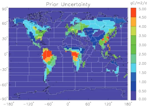
Given the above technical constraints, our choice of 200 regions should be seen as a compromise between optimality and feasibility. Figure 1 indicates the prior flux uncertainties used in the inversions and the region boundaries as white lines.
Over the oceans, a constant value of 0.2 g C m−2d−1is assumed for the uncertainty.
25
Over land, the uncertainty is defined from the annual ecosystem respiration field of the global carbon cycle model ORCHIDEE (Krinner et al., 2005), scaled to obtain a global total uncertainty around 4 Gt C yr−1(classical approach). At a weekly resolution, errors on any prior fluxes are likely to be correlated in time. We thus added exponentially
ACPD
10, 18561–18605, 2010CO2fluxes from various observing
systems
K. Hungershoefer et al.
Title Page
Abstract Introduction
Conclusions References
Tables Figures
◭ ◮
◭ ◮
Back Close
Full Screen / Esc
Printer-friendly Version
Interactive Discussion
Discussion
P
a
per
|
Dis
cussion
P
a
per
|
Discussion
P
a
per
|
Discussio
n
P
a
per
|
decreasing temporal correlations inCprior, with a decay time of four weeks. Given the relatively large size of each region, we did not impose spatial correlations between them. Accounting for the temporal correlations, we obtain a total land/ocean uncer-tainty of 4.4/0.6 Gt C yr−1.
To evaluate the benefit of several observation networks including satellite
instru-5
ments and potential surface networks described in Sect. 3, we will compute and com-pare the different error estimates (Cpost). More precisely, a typical error reduction (from the prior errorCprior) will be analysed for specific spatial and temporal scales The im-pact of combinations of observing systems is also analyzed. Note that with our analyt-ical approach Eq. (1), we can easily combine two observation networks, (O1,R1) and
10
(O2,R2), if there is no error correlations between the observations of the two networks
(i.e.R1 andR2 are independent). The product [HTR−1H] can be calculated separately for each observing system and then added.
The LMDZ transport model is used to compute the sensitivity of the concentrations to the surface fluxes of the 200 regions and 48 time periods (4 periods per month). The
15
model is derived from the general circulation model of the Laboratoire de M ´et ´eorologie Dynamique (LMDZ) (Sadourny and Laval, 1984, Hourdin et al., 2006) with a spatial resolution of 3.75◦ (longitude) and 2.5◦ (latitude) with 19 vertical levels. The 3-D con-centration fields (i.e. 96×73×19) were saved at each 6-h time step. In a second step, we extracted the results for each observing system described in the following section.
20
3 Observing systems
In this section, the nine observing systems to monitor atmospheric CO2concentrations, which are considered in this study, are described. These include,
– The current network of surface stations.
– The AIRS instrument onboard the Aqua satellite (Aumann et al., 2003).
ACPD
10, 18561–18605, 2010CO2fluxes from various observing
systems
K. Hungershoefer et al.
Title Page
Abstract Introduction
Conclusions References
Tables Figures
◭ ◮
◭ ◮
Back Close
Full Screen / Esc
Printer-friendly Version
Interactive Discussion
Discussion
P
a
per
|
Dis
cussion
P
a
per
|
Discussion
P
a
per
|
Discussio
n
P
a
per
|
– The SCIAMACHY instrument onboard the ENVISAT satellite (Bovensmann et al., 1999).
– The GOSAT satellite, which was launched in January 2009 (Kuze et al., 2009).
– The OCO satellite, which was lost during launch in February 2009 and is currently planned for rebuild (Crisp et al., 2004).
5
– The A-SCOPE mission, based on a lidar system that has been considered by the ESA but eventually not selected (Ingmann, 2009).
– Two extensions of the current surface network, named HYPOSURF-A and HYPOSURF-B, that could be build with the same funding as the A-SCOPE mis-sion.
10
For each of these systems, three kinds of information are required as input to the atmo-spheric transport inversions: The sampling (i.e. date, time, latitude and longitude), the vertical weighting function (or averaging kernel) that quantifies the vertical sensitivity of the observation, and a realistic estimate of the measurement uncertainty. The details of each topic are described in the remainder of this section.
15
3.1 Sampling
First, the method used to generate a realistic sampling for both the in-situ and satellite observations is described. The current ground network consists of more than 100 sta-tions scattered around the world. Some sample the concentrasta-tions at weekly, bi-weekly or monthly intervals, but there is a growing number of continuously measuring stations,
20
both in Europe and North America. However, it is clear that the many measurements that are acquired on a given day cannot be considered as independent. In addition, during the night and early morning, the low atmosphere is generally very stable so that surface fluxes are trapped in the first meters above ground and the measurements are representative of a very small area only. Night-time measurements are not useable
25
ACPD
10, 18561–18605, 2010CO2fluxes from various observing
systems
K. Hungershoefer et al.
Title Page
Abstract Introduction
Conclusions References
Tables Figures
◭ ◮
◭ ◮
Back Close
Full Screen / Esc
Printer-friendly Version
Interactive Discussion
Discussion
P
a
per
|
Dis
cussion
P
a
per
|
Discussion
P
a
per
|
Discussio
n
P
a
per
|
by current global scale inversions. For this reason, we consider that surface stations provide one independent measurement per day, during the afternoon. The measure-ments acquired from high towers are less affected by the night-time trapping and are representative of a larger area. They are therefore of higher value for the monitoring of carbon fluxes and we assume that they provide four independent measurements per
5
day, evenly distributed throughout the 24 h period (03, 09, 15, 21 local time).
Besides the existing surface network, two hypothetical network extensions that could be financed for the same price as a new satellite mission like A-SCOPE (∼200 Million Euros), are considered in this study. For the hypothetical network HYPOSURF-A, the money would be invested in the construction and maintenance of 418 new continuous
10
surface stations, using 41 already existing but currently un-instrumented towers. The second possible hypothetical network (HYPOSURF-B) would consist of towers only. In total, 168 stations could be financed, including 131 new towers and 38 currently existing towers being instrumented. The location of these potential stations were defined with the objective of an homogeneous coverage, but accounting for the ease of access
15
determined by the presence of a weather station.
Regarding satellite measurements, a rough description of the potential sampling can be obtained with a simple orbit geometry routine, accounting for the satellite altitude and the instrument scan angles. In addition, the cloud cover has to be taken into account, because the techniques used can only measure in a cloud-free atmosphere.
20
Using the MODIS Level 2 cloud mask (1 km resolution) of the year 2005, the presence of clouds in the field of view (FOV) was assessed for each potential sample generated by the orbitography routine (date and location). The potential observation is set as cloud contaminated and not used further whenever there is one or more cloudy MODIS pixels in the FOV. Hence, the number of clear-sky measurements depends on the
25
instrument field of view as the probability of cloud presence increases with the FOV size.
ACPD
10, 18561–18605, 2010CO2fluxes from various observing
systems
K. Hungershoefer et al.
Title Page
Abstract Introduction
Conclusions References
Tables Figures
◭ ◮
◭ ◮
Back Close
Full Screen / Esc
Printer-friendly Version
Interactive Discussion
Discussion
P
a
per
|
Dis
cussion
P
a
per
|
Discussion
P
a
per
|
Discussio
n
P
a
per
|
independent in the inversion system because of the large correlations among their errors and among the errors of the model that simulates them. Therefore, we apply a further sampling of the observation: For each satellite orbit, we kept only the best observation of each model grid box, even when many are available. As a result of this process, we have a set of (date, lat, lon) for each observing system. A typical coverage
5
for a month of observations is shown in Fig. 2.
3.2 Vertical weighting function
For the in-situ measurements, it is assumed that the observation is representative of the model layer corresponding to the station’s altitude. For surface stations, it is the lowermost layer in most cases, with a few exceptions over hilly terrain. Airborne
sam-10
ples are used at the flight level. In case of towers, a typical height of 200 m is added to the station’s altitude.
Satellite measurements are more difficult to handle, because the measured CO2 concentration represents a weighted average over the whole vertical column. In gen-eral, the vertical weighting function, w(P), is used to compute the column weighted
15
average, CO2, from the concentration profile CO2(P) provided by the transport model:
CO2= Psurf
Z
0
w(P)·CO2(P)d P , (4)
where P is the atmospheric pressure. These weighting functions, derived from ra-diative transfer simulations, depend on several geophysical parameters such as the temperature profile, the surface albedo, or the presence of aerosol particles, as well
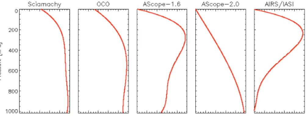
20
as the observing geometry. However, for typical conditions (i.e. excluding the marginal cases with high aerosol contents or very low surface reflectances), the variations are relatively small. For the sake of simplicity, a constant weighting function is used for each of the remote sensing instruments here. They are shown in Fig. 3.
ACPD
10, 18561–18605, 2010CO2fluxes from various observing
systems
K. Hungershoefer et al.
Title Page
Abstract Introduction
Conclusions References
Tables Figures
◭ ◮
◭ ◮
Back Close
Full Screen / Esc
Printer-friendly Version
Interactive Discussion
Discussion
P
a
per
|
Dis
cussion
P
a
per
|
Discussion
P
a
per
|
Discussio
n
P
a
per
|
SCIAMACHY, OCO and GOSAT (not shown) are based on the same measurement principle (i.e. differential absorption spectroscopy) and show very similar weighting functions, with some differences that result from the spectral resolution. In all three cases, the weighting function is fairly constant throughout the troposphere, and de-creases in the higher levels of the atmosphere. As a consequence, these instruments
5
may provide a concentration estimate that is close to the tropospheric average. The weighting function from thermal infrared instruments (such as AIRS or IASI) is very different, as can be seen in Fig. 3. It peaks between 200 and 300 hPa and the relative contribution of the lower half of the atmosphere (below 500 hPa) is only on the order of 15%. Active sensing systems are also based on the differential absorption techniques
10
but use a single pair of wavelengths only. The weighting function depends very much on the absorbing channel wavelength. For CO2, the weak absorption band at 1.6 µm and the strong absorption band at 2.0 µm turned out to be appropriate (Koch et al., 2004; Joly et al., 2009). The weighting function at 1.6 µm peaks at 300 hPa, albeit with a significant contribution from all levels down to the surface, while the weighting
15
function at 2.0 µm is almost proportional to the pressure. For the monitoring of surface fluxes, the latter appears most favourable, as it is the most sensitive to the atmospheric boundary layer where local surface fluxes have the largest impact. In our study, both possibilities are investigated. To distinguish them, the terms A-SCOPE-2.0 (operating at 2 µm) and A-SCOPE-1.6 (λ=1.6 µm) are used.
20
3.3 Measurement uncertainty
The measurement uncertainty, or error, is also a critical parameter to assess the po-tential impact of an observing system. The measurement uncertainty concerns the difference between simulated and observed quantities and thus contains errors in both atmospheric transport and satellite retrieval. The uncertainty is difficult to determine
25
ACPD
10, 18561–18605, 2010CO2fluxes from various observing
systems
K. Hungershoefer et al.
Title Page
Abstract Introduction
Conclusions References
Tables Figures
◭ ◮
◭ ◮
Back Close
Full Screen / Esc
Printer-friendly Version
Interactive Discussion
Discussion
P
a
per
|
Dis
cussion
P
a
per
|
Discussion
P
a
per
|
Discussio
n
P
a
per
|
simulations performed by various groups in the context of an ESA-funded study (Br ´eon et al., 2009) analyzing the impact of both instrument noise and geophysical parame-ters. For missions using the differential absorption technique, both passive and active, the surface reflectance is a key parameter. Over the oceans, we used the statistics of glint reflectances derived from POLDER observations (Br ´eon and Henriot, 2006) and
5
we accounted for the observation geometry. Over land, we used the MODIS albedo product, which is a good approximation of the reflectance for typical viewing condi-tions. For the particular case of A-SCOPE, the albedo was multiplied by a factor of 2, because the backscatter (or Hot-Spot) effect has to be taken into account for the lidar viewing geometry (Br ´eon et al., 2002).
10
For AIRS, it was found that the random error is mostly a function of latitude (related to the atmospheric temperature profile). Radiative transfer simulations indicate that the error on the column weighted CO2 is close to 2.3 ppm in the tropics and strongly increases towards the polar regions. For our study, we make a simple approximation for the errorσAIRS:
15
σAIRS=2.3+4·(lat/90)2 [ppm]. (5)
For OCO, radiative transfer simulations indicate that the error varies with the sun and/or viewing zenith angle, the aerosol optical depth and the surface reflectance. In short, the instrument performance is best for a high reflectance, while the presence of aerosol generates some noise, especially if the atmospheric path is long. Based on a large
20
number of simulations with varying conditions (observing geometry, surface and atmo-spheric conditions), the following formula was derived
σOCO=0.6+0.1·mτaer/Alb1.6 [ppm]. (6)
The parameterm is the airmass (m=cos(θs)−1
+cos(θv)−1) which is a function of the solar zenith angle (θs) and the viewing angle (θv). τaer is the aerosol optical thickness
25
and Alb1.6is the surface albedo at 1.6 µm.
ACPD
10, 18561–18605, 2010CO2fluxes from various observing
systems
K. Hungershoefer et al.
Title Page
Abstract Introduction
Conclusions References
Tables Figures
◭ ◮
◭ ◮
Back Close
Full Screen / Esc
Printer-friendly Version
Interactive Discussion
Discussion
P
a
per
|
Dis
cussion
P
a
per
|
Discussion
P
a
per
|
Discussio
n
P
a
per
|
SCIAMACHY uses the same measurement technique as OCO, but with a larger random error due to its poor spectral resolution and signal-to-noise ratio. Therefore, the same formula as for OCO, but with coefficients twice as large, is used here:
σSCIA=1.2+0.2·mτaer/Alb1.6 [ppm]. (7)
For GOSAT, uncertainty estimates provided by the algorithm development team and
5
discussed in Chevallier et al. (2009) describe the error as a function of the albedo and the viewing angle:
σGOSAT= s
0.26 Alb1.6cosθs
2
+1.22 [ppm]. (8)
ASCOPE’s measurement technique has the advantage that the error does not depend on the presence of aerosol or the sun angle. Besides, the viewing geometry is limited to
10
nadir viewing. The main variable to define the error is the surface reflectance. Radiative transfer simulations indicate that, for a lidar working at 1.6 µm, the typical error can be fitted by:
σASCOPE 1.6= q
(0.35−1.25 Back1.6)2+0.181 [ppm]. (9)
The lidar backscatter (Back1.6) is derived from the scene reflectance through a simple
15
division byπ(reflectance to backscatter). To obtain an error estimate for a lidar at 2 µm, we simply multiply the 1.6 µm error by a factor of two. This factor of 2 is consistent with the results of an extended error analysis (see Br ´eon et al., 2009) and allows comparing the impact of weighting function and random error (see Sect. 4).
Transport model errors are not considered for the satellite observing systems here.
20
A recent study of Houweling et al. (2010) shows that these model errors are an impor-tant factor limiting the accuracy of the determination of CO2fluxes.
ACPD
10, 18561–18605, 2010CO2fluxes from various observing
systems
K. Hungershoefer et al.
Title Page
Abstract Introduction
Conclusions References
Tables Figures
◭ ◮
◭ ◮
Back Close
Full Screen / Esc
Printer-friendly Version
Interactive Discussion
Discussion
P
a
per
|
Dis
cussion
P
a
per
|
Discussion
P
a
per
|
Discussio
n
P
a
per
|
measurements may not be representative of CO2concentration at the model grid scale used for the inversion. Also, vertical transport is more variable among transport models (Gurney et al., 2002) and probably more error-prone. It will likely impact simulations of one level at the surface more than weighted vertical integrals. Atmospheric transport simulations at high spatial resolution showed that the sub-grid variability depends very
5
much on the location and is largest close to major CO2sources and sinks. Following Roedenbeck (2005), and based on high-resolution simulations, we set an error that depends on the site:
– Remote sites (islands, deserts, Antarctica): 1.0 ppm
– Shore sites with mixed Ocean/continent influence: 1.5 ppm
10
– Continental site with complex circulation and fluxes: 3.0 ppm
– Mountain site (on continents); simpler circulation: 1.5 ppm. The error associated with each station can be seen in Fig. 2a.
4 Results
21 observing systems have been tested. Besides the 9 single observing systems listed
15
in Sect. 3, we also considered eight combinations of the existing surface network with one satellite, and four combinations of the existing surface network, AIRS and one other satellite.
The analytical flux inversion yields the posterior uncertainty (σi) for each week and region over one year, together with the correlation terms. Since there is no reason
20
to focus on one particular week i, we first discuss the quadratic-mean weekly error, defined as
¯
σweek= s
1
N
X
i
σi2, (10)
ACPD
10, 18561–18605, 2010CO2fluxes from various observing
systems
K. Hungershoefer et al.
Title Page
Abstract Introduction
Conclusions References
Tables Figures
◭ ◮
◭ ◮
Back Close
Full Screen / Esc
Printer-friendly Version
Interactive Discussion
Discussion
P
a
per
|
Dis
cussion
P
a
per
|
Discussion
P
a
per
|
Discussio
n
P
a
per
|
whereN is the number of periods. Another option would be the mean weekly error, but the quadratic mean defined in Eq. (10) gives more weight to the periods with the largest uncertainties, i.e. when there is significant knowledge to be gained. Applying Eq. (10) to the prior and the posterior uncertainty, the typical weekly error reduction ERweekis obtained by
5
ERweek=1− ¯
σweekpost
¯
σweekprior
. (11)
The error reduction takes values between 0 and 1. High values indicate that the con-sidered observing system is well suited to improve our knowledge on the CO2surface fluxes over the considered region. For each observing system simulation experiment (OSSE) we will concentrate on a few major characteristics of the posterior error
covari-10
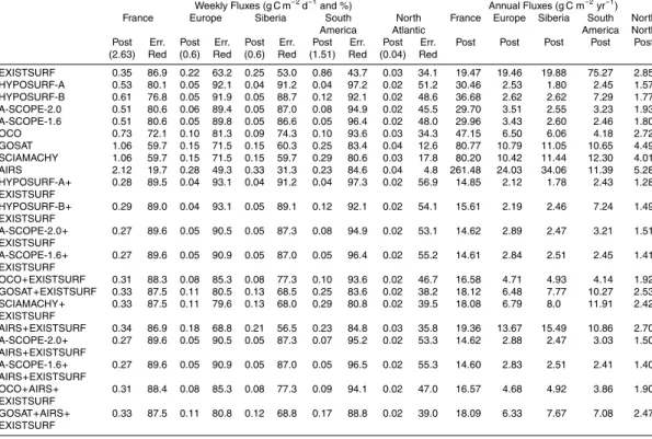
ance matrix. First, the number of observations for the different observing systems are analysed in Sect. 4.1. The typical weekly error reduction maps are then discussed in Sect. 4.2 while the posterior annual flux uncertainties are shown in Sect. 4.3. For a few regions, Table 1 provides the results (prior and posterior uncertainties, error reduction) for all 21 OSSEs. The five regions that were selected for Table 1 are France, Europe,
15
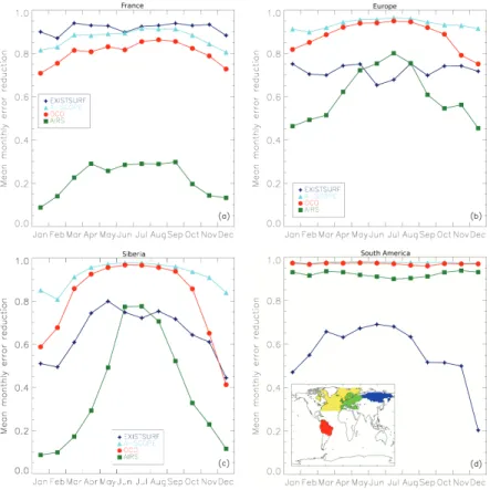
Siberia, Tropical South America and North Atlantic. France and Europe were selected for the dense surface network over Western Europe. Siberia and South America are areas of concern with regard to climate change with very limited in-situ monitoring in South America. For ocean, we choose the North Atlantic north of 30◦N, a region where recent observations suggest a significant decrease of the annual carbon sink.
20
The analytic method makes it possible to combine the statistical results for areas that aggregate several of the pre-defined 200 regions. It is then possible to analyze how the uncertainties (or the error reduction) vary with the spatial scale. In Table 1, France, as a sub-area of Europe, can be used for that purpose. Except for France, the regions in Table 1 are based on the aggregation of several of the original 200 regions as their
25
ACPD
10, 18561–18605, 2010CO2fluxes from various observing
systems
K. Hungershoefer et al.
Title Page
Abstract Introduction
Conclusions References
Tables Figures
◭ ◮
◭ ◮
Back Close
Full Screen / Esc
Printer-friendly Version
Interactive Discussion
Discussion
P
a
per
|
Dis
cussion
P
a
per
|
Discussion
P
a
per
|
Discussio
n
P
a
per
|
It is necessary to stress that the posterior errors and error reductions depend on many hypothesis, in particular regarding the prior flux uncertainties, their spatial and temporal covariances, and the choice of the 200 “eco-regions” that are assumed homo-geneous in terms of CO2 flux errors. Hence, we have more confidence in the relative performance of the various observing systems that are analyzed than in the absolute
5
values (see discussion Sect. 5.1).
4.1 Number of observations
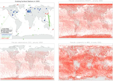
The total number of observations during the whole year varies between 26 000 (exist-ing surface network) and 928 000 (AIRS). The geographical distribution of the exist(exist-ing surface stations and the pseudo-observations obtained by A-SCOPE, OCO and AIRS
10
in January are displayed in Fig. 2. Although the surface network measurements have a high temporal resolution, the spatial coverage is much poorer compared to the satel-lite observations. As can be seen in Fig. 2, the sampling is very limited over South America, Africa and tropical Asia. On the contrary, A-SCOPE and AIRS result in the best global coverage because they are able to perform measurements during day and
15
night. In contrast, no OCO measurements are possible in the high latitudes of the Northern Hemisphere in January. The same is true for SCIAMACHY and GOSAT (not shown). AIRS has the best global coverage both because it has wide scanning capa-bilities and because it is not affected by low clouds.
4.2 Weekly fluxes
20
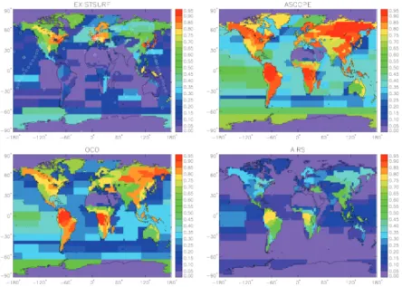
Global maps of the typical weekly error reduction (see Eq. 10) for four OSSEs, namely the existing surface network (EXISTSURF), A-SCOPE-2.0, OCO and AIRS are shown in Fig. 4. Table 1 provides the weekly fluxes of all 21 OSSEs for four large regions (Europe, Siberia, South America and North Atlantic) which are the sum of several individual regions.
25
ACPD
10, 18561–18605, 2010CO2fluxes from various observing
systems
K. Hungershoefer et al.
Title Page
Abstract Introduction
Conclusions References
Tables Figures
◭ ◮
◭ ◮
Back Close
Full Screen / Esc
Printer-friendly Version
Interactive Discussion
Discussion
P
a
per
|
Dis
cussion
P
a
per
|
Discussion
P
a
per
|
Discussio
n
P
a
per
|
As expected, all observing systems provide information on the carbon fluxes and this information leads to an error reduction on the weekly fluxes. For the current surface network, the error reduction is the largest in regions with a dense coverage (Western Europe, North-eastern US and Korea-Japan). Note the white circles in Fig. 4 that show the location of the stations. In such areas, the error reduction is larger than 80%. In
5
a small region like France (Table 1), the surface network results in the highest error reduction (87%) of all observing systems but, as the area increases (e.g. from France to Europe, Table 1), a higher error reduction is achieved by all satellite measurements, except AIRS. For other vegetated areas with a sparser surface network, the error re-duction is on the order of 50%. Over continents such as Africa or South-America that
10
are very sparsely covered, the error reduction is even lower. Over the oceans, the sur-face observing network provides limited information to improve the knowledge on the carbon fluxes.
Among the satellite systems, the A-SCOPE instrument provides the best constraint on surface carbon fluxes. The obtained error reductions are larger than 75% over
15
vegetated areas and reach values between 30% and 50% over the oceans. OCO shows similar performance to the lidar mission over the tropics, but somewhat lower over the high latitudes, probably because of a lack of measurements during winter. In spite of the good spatial coverage of the AIRS instrument (Fig. 2), the error reduction of this system is much smaller than that of A-SCOPE and OCO. The reason is the higher
20
measurement uncertainty, especially outside the Tropics, and the vertical weighting function, which is not sensitive enough to the atmospheric boundary layer and therefore weakly related to the surface fluxes.
As can be seen in Table 1, the hypothetical network extension HYPOSURF- A gives the highest error reduction of all observing systems for Europe, Siberia, South
Amer-25
ACPD
10, 18561–18605, 2010CO2fluxes from various observing
systems
K. Hungershoefer et al.
Title Page
Abstract Introduction
Conclusions References
Tables Figures
◭ ◮
◭ ◮
Back Close
Full Screen / Esc
Printer-friendly Version
Interactive Discussion
Discussion
P
a
per
|
Dis
cussion
P
a
per
|
Discussion
P
a
per
|
Discussio
n
P
a
per
|
possible extensions of the current network (they do not include the current network). With already a high density over Western Europe for the current network few new sta-tions are thus foreseen over this area. If the existing surface network is combined with each hypothetical extension, the maximal error reduction of all observing systems is reached for Europe, Siberia and the North Atlantic. Hence, both hypothetical
net-5
work extensions are a promising strategy for CO2 monitoring to be compared against satellite investment (see discussion below).
Inter-comparing the error reduction of the different satellites considered in our study shows that both A-SCOPE cases are performing best, followed by OCO. The error re-duction for GOSAT and SCIAMACHY are already significantly lower. The lowest error
10
reduction was found for AIRS, except in the tropics where AIRS results in a better er-ror reduction than GOSAT. For the two A-SCOPE cases similar erer-ror reductions are obtained in France, Europe and Siberia. For South America, A-SCOPE-1.6 is better than A-SCOPE-2.0. In general, the better weighting function of A-SCOPE-2.0 (peaked towards the surface) is compensated by the better precision of A-SCOPE-1.6. Over
15
South America, atmospheric convection mixes the air on a deep layer. As a conse-quence, the weighting function of A-SCOPE-2.0 is less of an advantage, and the better precision of A-SCOPE-1.6 drives the overall performance.
Combining the measurements of one satellite with the surface network increases the total error reduction in areas with surface stations (Table 1). E.g., an error reduction of
20
89.6% is obtained for the combination of A-SCOPE and EXISTSURF for France. This is higher compared to the error reduction of 80.6% and 86.9% obtained for A-SCOPE and EXISTSURF as individual observing systems. As expected, the combination does not result in a higher error reduction in a region like South America where no surface measurements are available. In this case, the posterior uncertainties and the error
25
reductions are the same as when using the satellite measurements alone. Table 1 also shows that the additional consideration of AIRS does not improve the results ob-tained over Europe and Siberia for the combination of the existing surface network with A-SCOPE, OCO and GOSAT, respectively. AIRS adds some information only in
ACPD
10, 18561–18605, 2010CO2fluxes from various observing
systems
K. Hungershoefer et al.
Title Page
Abstract Introduction
Conclusions References
Tables Figures
◭ ◮
◭ ◮
Back Close
Full Screen / Esc
Printer-friendly Version
Interactive Discussion
Discussion
P
a
per
|
Dis
cussion
P
a
per
|
Discussion
P
a
per
|
Discussio
n
P
a
per
|
the Tropics. Again, this is understood as the effect of deep convection that links the surface and the mid and upper troposphere which AIRS is sensitive to.
To investigate the advantages and disadvantages of the different observing systems, it is also interesting to look at the change of the performance within one year. There-fore, time series of the monthly error reduction (accounting for covariances between
5
weekly errors) for the existing surface network, A-SCOPE-2.0, OCO and AIRS are shown in Fig. 5. We observe significant seasonal variations for the four selected re-gions that reflect seasonal variations of the prior errors, of the number of observations, and of seasonal variations in the atmospheric vertical mixing (probably more crucial for the surface networks). Altogether, A-SCOPE is performing best, with the highest
10
error reduction for all regions, except France where the existing surface network dom-inates, and with the smallest monthly variations. In the case of South America, Fig. 5 emphasises the very good performance of OCO throughout the year, while the surface network shows low error reduction and a seasonal pattern linked to changes in atmo-spheric mixing. For Europe and Siberia, the monthly error reduction of OCO in the
15
summer months is almost as high as the one for A-SCOPE. The strong annual cycle in the error reduction for these two regions reflects that of the prior uncertainties (larger flux uncertainties in summer) modulated by the number of measurements of each ob-serving system. In winter the lidar-based A-SCOPE mission provides more information than OCO’s because the sun is too low to permit measurements by the passive
tech-20
nique of the OCO mission. As already seen, AIRS’s performance is only competitive with the other satellites in South America. In other regions, the performance is signif-icantly worse than that of the other satellite systems, and shows an annual cycle that reflects the prior uncertainties.
4.3 Annual fluxes
25
ACPD
10, 18561–18605, 2010CO2fluxes from various observing
systems
K. Hungershoefer et al.
Title Page
Abstract Introduction
Conclusions References
Tables Figures
◭ ◮
◭ ◮
Back Close
Full Screen / Esc
Printer-friendly Version
Interactive Discussion
Discussion
P
a
per
|
Dis
cussion
P
a
per
|
Discussion
P
a
per
|
Discussio
n
P
a
per
|
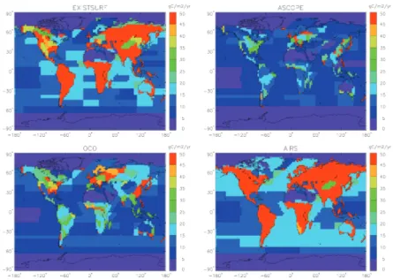
in Europe and North America). In these regions, e.g., France, none of the satel-lite systems attains such a low posterior uncertainty (see numbers in Table 1). On the other hand, the posterior uncertainty of the existing surface network amounts to more than 45 g C m−2yr−1in South America, Siberia and Southern Africa, and around 15 g C m−2yr−1over the ocean. Over vegetated areas the A-SCOPE posterior error is
5
in the range of 10 to 30 g C m−2yr−1. In most ocean regions the uncertainty is below 10 g C m−2yr−1. For OCO the posterior errors are slightly larger with values between 15 and 50 g C m−2yr−1over land and up to 15 g C m−2yr−1over the oceans.
Annual flux errors for larger regions (i.e. aggregation of few individual regions) such as Europe, Siberia, South America and the North Atlantic are also given in Table 1.
10
The computation of these errors accounts for all spatial covariances inCpost (Eq. 3). The resulting annual flux uncertainties appear to be much smaller than the uncertainty of the individual regions shown in Fig. 6. For both A-SCOPE cases, the error per unit area decreases by a factor 8–9 between France and Europe (from around 30 to 3.5 g C m−2yr−1). This reduction partly results from negative error correlations. Without
15
these correlation terms the error would reduce to only 5.2 g C m−2yr−1as a results of aggregating regions with independent errors. The change from 5.2 to 3.5 g C m−2yr−1 becomes important when assessing the potential of an observing system to constrain annual fluxes as a function of spatial scale (see Sect. 5.1). It highlights the importance of negative error correlations between adjacent regions. As can be seen in Table 1,
20
an extension of the surface network is encouraging. HYPOSURF-A results in the low-est posterior error of all observing systems for Europe, Siberia and South America. A-SCOPE and OCO are much better than the other satellites. GOSAT and SCIA-MACHY produce posterior errors about twice those of A-SCOPE and OCO. In South America the performance of AIRS is comparable to that of GOSAT and SCIAMACHY,
25
while in Europe and Siberia the posterior error achieved with AIRS is around 25 and 35 g C m−2yr−1, respectively. The existing surface network combined with A-SCOPE significantly decreases the annual error over France (region with a dense network). The same is true for the combination of EXISTSURF with the surface network extensions.
ACPD
10, 18561–18605, 2010CO2fluxes from various observing
systems
K. Hungershoefer et al.
Title Page
Abstract Introduction
Conclusions References
Tables Figures
◭ ◮
◭ ◮
Back Close
Full Screen / Esc
Printer-friendly Version
Interactive Discussion
Discussion
P
a
per
|
Dis
cussion
P
a
per
|
Discussion
P
a
per
|
Discussio
n
P
a
per
|
For ocean, the posterior error decreases from around 7(12) g C m−2yr−1, for an indi-vidual region of North Atlantic (East Atlantic, Fig. 6) to around 2(3) g C m−2yr−1, for the whole North Atlantic (>30◦N) for A-SCOPE-20 and the surface network, respectively.
5 Discussion
Before discussing the implications of our results for CO2observing systems in Sect. 5.2
5
there are several caveats which must be explored.
5.1 How robust is the comparison?
We see from Eq. (3) that the error reduction depends on the uncertainty covariances for prior flux estimates and measurements plus the matrix representing transport. The choice of source resolution is critical as it underlies the two of them.
10
Source resolution:
Even though we perform all OSSEs with the same set-up, the source resolution will impact the results. Our set-up, with 200 regions tiling the globe, may be viewed as not representing the current state of the art in source/sink inversions. These are usually performed at gridpoint resolution with the imposition of evanescent correlations among
15
pixels, although few recent studies choose to resolve the fluxes for large “ecosystem regions” (i.e. CarbonTracker, Peters et al., 2007). These correlation lengths are largely unknown and, like all other aspects of the prior statistics, should be informed by inde-pendent data (e.g., Chevallier et al., 2006).
The source resolution also enters the problem via the influence or footprint of each
20
measurement. In an inversion with fixed regions, the whole region is constrained by a single measurement while the same measurement applies a less rigid constraint us-ing gridpoints and correlations. Given the sum of squares nature of the posterior Hes-sian (Eq. 3) there are sharply diminishing returns as a region is oversampled. Imagining the limiting case of infinite prior uncertainty and no transport (i.e. each measurement
ACPD
10, 18561–18605, 2010CO2fluxes from various observing
systems
K. Hungershoefer et al.
Title Page
Abstract Introduction
Conclusions References
Tables Figures
◭ ◮
◭ ◮
Back Close
Full Screen / Esc
Printer-friendly Version
Interactive Discussion
Discussion
P
a
per
|
Dis
cussion
P
a
per
|
Discussion
P
a
per
|
Discussio
n
P
a
per
|
only sees fluxes from its own region) we see that the posterior uncertainty will remain infinite for regions without a station. The number of surface stations required hence de-pends critically on the source resolution (and potential correlations). This dependence is much weaker for satellite measurements. As a direct consequence, we obtain for instance a larger error reduction for large ocean basins compared to smaller adjacent
5
basins (Fig. 4), with corresponding lower posterior errors (Fig. 6).
Transport resolution:
The transport model resolution also enters the problem. The use of correlations (or large regions) avoids the dominance of the near-field noted by Bocquet (2005) and Gerbig et al. (2009). Our choice of sampling for the satellite measurements (Sect. 3.1)
10
is, however, strongly dependent on model resolution. The implication that the high-resolution soundings of instruments like OCO or A-SCOPE contain errors with respect to the transport model completely correlated at 250 km (the approximate north-south extent of an LMDZ gridbox) and completely uncorrelated beyond this has no geophys-ical basis. It is most likely that there is extra information at smaller scales and that this
15
information would strengthen the constraint offered by these instruments as resolution was increased.
The performance of the surface network is also affected by capabilities of the trans-port model. The term representativeness describes the extent to which a given mea-surement represents a model gridbox. It is different from the problem of grouping pixels
20
into regions discussed above. Representativeness errors form part of the uncertainty covariance for data (Rin Eqs. 2 and 3). They are likely larger for larger gridboxes and more heterogeneous sources. Corbin et al. (2009) has shown that they are not large for column-integrated measurements taken in swaths over a gridbox (a measurement reminiscent of a satellite) but the problem is less widely studied for surface
measure-25
ments.
Representativeness errors will certainly decrease as model resolution increases. So, probably, will errors in transport. Geels et al. (2006) and Law et al. (2008) have both shown that higher resolution models, particularly mesoscale models, can capture much
ACPD
10, 18561–18605, 2010CO2fluxes from various observing
systems
K. Hungershoefer et al.
Title Page
Abstract Introduction
Conclusions References
Tables Figures
◭ ◮
◭ ◮
Back Close
Full Screen / Esc
Printer-friendly Version
Interactive Discussion
Discussion
P
a
per
|
Dis
cussion
P
a
per
|
Discussion
P
a
per
|
Discussio
n
P
a
per
|
more of the information available from continuous surface measurements. Inversion studies such as Lauvaux et al. (2009) have shown that this information can provide an improved constraint for surface fluxes. Initial tests (R. Engelen (ECMWF), personal communication, 2010) suggest that models running at tens of kilometers resolution could use far more than the one daily measurement from surface stations or four from
5
towers used here, improving the performance of the surface network.
Prior flux error covariance:
The prior covariance matrix (Cprior) that we have defined neglects key characteristics of the carbon cycle and should still be considered a crude approximation. Indeed, the er-ror correlation terms are difficult to assess and are only partially accounted for inCprior.
10
We use “eco-regions” for the spatial domain and only positive temporal correlations for the time domain (exponential decay with a time constant of one month). However, neg-ative correlations between summer and winter flux errors for instance, are not included (an excess of carbon uptake during the growing season is likely to enhance the respi-ration in the following months). Omitting these terms leads to an overall prior annual
15
land and ocean error budget of 4.4 and 0.6 Gt C yr−1, respectively, which is unrealisti-cally large for land given our knowledge of the carbon cycle. As a direct consequence, the posterior budget is likely overestimated (i.e. 0.73 and 0.47 for land and ocean with the EXISTSURF observing system). We expect this to have larger effects on the ab-solute errors discussed throughout the paper than the relative performance of different
20
systems.
Data uncertainty:
The final critical input to the calculations is the data uncertainty covariance R. We stress again that this represents uncertainty in the model-data mismatch and so con-tains components from the measurement itself (already the product of an inversion
25
ACPD
10, 18561–18605, 2010CO2fluxes from various observing
systems
K. Hungershoefer et al.
Title Page
Abstract Introduction
Conclusions References
Tables Figures
◭ ◮
◭ ◮
Back Close
Full Screen / Esc
Printer-friendly Version
Interactive Discussion
Discussion
P
a
per
|
Dis
cussion
P
a
per
|
Discussion
P
a
per
|
Discussio
n
P
a
per
|
possibility that confounding influences on satellite retrievals such as aerosol and thin clouds could induce coherent errors beyond one gridbox, especially in high latitudes where gridboxes are small. This would decrease the information content of satellite data.
For the surface network the problem rests on transport error. It is generally thought
5
that, with higher uncertainty in vertical transport, this component of model error should be larger for surface than column-integrated measurements. Our specification of R
takes this into account but we have little way of knowing whether we have captured the difference successfully and even less of predicting how these differences will compare as models improve.
10
Overall, our study has a range of limitations when comparing satellite and surface systems. These may compensate or exacerbate each other, precluding an unambigu-ous result. Two things can be concluded firmly however. First the choice of measure-ment approaches depends on the quality of the tools we use to interpret them. Given all above limitations, we guess that current set-up likely favours the surface network.
15
Second, the combination of both observing systems is likely to bring cross constraint in the optimization process and thus to decrease the impact of each system’s biases and provide the most precise flux estimates. Additionally we suggest that a large surface network expansion, although probably difficult to achieve over the tropics, would require significant model improvement (representativeness and transport errors), while for the
20
foreseen satellite instruments the precision of the measurements is crucial although still largely debated.
Concerning the rating of the different satellites, it was shown in Sect. 4, that they do not perform equally and that A-SCOPE provides the best information on the surface fluxes among them. The information provided by GOSAT is less compared to OCO or
25
A-SCOPE and is similar to that of SCIAMACHY. This result may seems surprising con-sidering the fact that it is a carbon-dedicated instrument, but this follows directly from the cautious precision estimates provided by the GOSAT team. This situation may well change as confidence in GOSAT retrieval algorithms grows. AIRS does a poor job for
ACPD
10, 18561–18605, 2010CO2fluxes from various observing
systems
K. Hungershoefer et al.
Title Page
Abstract Introduction
Conclusions References
Tables Figures
◭ ◮
◭ ◮
Back Close
Full Screen / Esc
Printer-friendly Version
Interactive Discussion
Discussion
P
a
per
|
Dis
cussion
P
a
per
|
Discussion
P
a
per
|
Discussio
n
P
a
per
|
providing additional information on the carbon fluxes in particular over mid and high latitude where the measurements are of much lower quality than over the tropics. The ranking of the different satellite systems is directly linked to the number of measure-ments, the assumed errors and the vertical weighting functions. The ranking of the satellite systems is likely to be more robust than the differences between the surface
5
and the satellite observing systems, given the limitations discussed above.
5.2 Potential of the observing systems and carbon cycle targets
The results presented above demonstrate that all observing systems discussed in this paper may improve our knowledge of the carbon cycle. Indeed, the amplitude of the error reduction on the regional fluxes is significant and reaches values up to 90%.
How-10
ever, such error reduction (or more directly the posterior error) depends on the inverse set-up. Furthermore, it may be insufficient to answer key questions of the carbon cycle that may require even lower errors. The following discussion is based on the absolute posterior error rather than the error reduction and we stress again the sensitivity of this diagnostic to various inputs (see Sect. 5.1). We note that the scientific
commu-15
nity tends to use an ensemble of inversions (varying several components) to define a more robust error diagnostic (see for instance the TransCom experiment, Gurney et al., 2003). Being aware of these limitations, it is still interesting to attempt to quantify the requirements for some key questions, and assess whether these requirements can be met by the various observing systems that we have defined. We have identified
20
four key questions: one of them focuses on the weekly/monthly fluxes, while the other ones focus on annual fluxes. The requirements are discussed below and summarized in Table 2.
Land-Vegetation dynamics:
Vegetation dynamic models are developed to understand the functioning of
ecosys-25