Data-Driven Engineering of Social Dynamics: Pattern Matching and Profit Maximization.

Data-Driven Engineering of Social Dynamics:

Pattern Matching and Profit Maximization

Huan-Kai Peng1*, Hao-Chih Lee2, Jia-Yu Pan3, Radu Marculescu1

1Department of Electrical and Computer Engineering, Carnegie Mellon University, Pittsburgh, Pennsylvania, United States of America,2Department of Biomedical Engineering, Carnegie Mellon University, Pittsburgh, Pennsylvania, United States of America,3Google Inc., Mountain View, California, United States of America

*pumbaapeng@gmail.com

Abstract

In this paper, we define a new problem related to social media, namely, the data-driven engineeringof social dynamics. More precisely, given a set of observations from the past, we aim at finding the best short-term intervention that can lead to predefined long-term out-comes. Toward this end, we propose a general formulation that covers two useful engineer-ing tasks as special cases, namely,pattern matchingandprofit maximization. By

incorporating a deep learning model, we derive a solution using convex relaxation and qua-dratic-programming transformation. Moreover, we propose a data-driven evaluation method in place of the expensive field experiments. Using a Twitter dataset, we demonstrate the effectiveness of our dynamics engineering approach for both pattern matching and profit maximization, and study the multifaceted interplay among several important factors of dynamics engineering, such as solution validity, pattern-matching accuracy, and interven-tion cost. Finally, the method we propose is general enough to work with multi-dimensional time series, so it can potentially be used in many other applications.

1 Introduction

The two distinct goals in scientific inquiry are understanding and engineering. Understanding is often associated with system analysis, modeling, and prediction, whereas engineering is often associated with design, control, and optimization. While understanding is fundamentally important, engineering often acts as the trigger for technological revolution. For example, although Kirchhoff discovered the basic circuit laws in 1845, VLSI revolution came only when the CMOS technology and its tool chain were invented more than a century later.

In the context of social networks, or more specifically,social dynamics, one would wonder what a similar triggering technology would be. Research in social dynamics has examined pat-tern discovery [1–4], modeling [5–7], and prediction [8–13]. Most, if not all, of this work, how-ever, leans toward the understanding side. In contrast, the engineering side, which is more about control and targeted intervention of social dynamics, is far less explored. Even so, we argue that many engineering questions, if answered, have the potential to revolutionize the OPEN ACCESS

Citation:Peng H-K, Lee H-C, Pan J-Y, Marculescu R (2016) Data-Driven Engineering of Social Dynamics: Pattern Matching and Profit Maximization. PLoS ONE 11(1): e0146490. doi:10.1371/journal.pone.0146490

Editor:Sergio Gómez, Universitat Rovira i Virgili, SPAIN

Received:May 23, 2015

Accepted:December 17, 2015

Published:January 15, 2016

Copyright:© 2016 Peng et al. This is an open access article distributed under the terms of the

Creative Commons Attribution License, which permits unrestricted use, distribution, and reproduction in any medium, provided the original author and source are credited.

Data Availability Statement:The authors do not own the data. The Twitter dataset is owned and provided by Professor Jure Leskovec from Stanford University. The Twitter data set used in this study is available athttps://snap.stanford.edu/data/bigdata/ twitter7/tweets2009-12.txt.gz. The citation is: J. Yang, J. Leskovec. Temporal Variation in Online Media. ACM International Conference on Web Search and Data Mining (WSDM‘11), 2011. Interested researchers can also request the data set directly from Professor Leskovec (viajure@cs.stanford.edu).

area of social networks. To illustrate, let us consider the following two engineering questions for social dynamics:

• Pattern matching: How can we manipulate social dynamics to follow a certain (successful) pattern in the future?

• Profit maximization: How can we maximize the long-term popularity of a hashtag using low-cost targeted intervention in the short-term?

The answers to such questions can impact significantly many aspects of social-media applica-tions, e.g., marketing [14], politic [15], social mobilization [16], and disaster management.

Consequently, in this paper, we focus precisely on data-driven engineering approaches of social dynamics, where the main challenges are three-fold:

1. Define a problem formulation that is general enough to cover arange ofengineering tasks.

2. Design a solution that is both reliable and efficient.

3. Provide a method to evaluate the quality of our solution using historical data, instead of using expensive and time-consumingfield experiments[17].

To the best of our knowledge, this is the first work that offers the following contributions:

1. Dynamics-engineering framework: We propose a framework for data-driven dynamics engi-neering that consists of three components. First, we propose a general formulation, which includes both pattern matching and profit maximization as special cases. Second, using a deep-learning model, we derive a solution based on convex relaxation and quadratic-pro-gramming transformation, which is efficient and is guaranteed to converge to the global optimum. Finally, we propose a data-driven evaluation method instead of time-consuming and expensive field experiments [17].

2. Experimental studies of pattern matching vs. profit maximization: We experiment on both engineering tasks, i.e., pattern matching and profit maximization, using a Twitter dataset. For each task, we report and analyze the interesting tradeoffs that are critical to real-world dynamics engineering applications, including solution validity, pattern mismatch, interven-tion cost, and outcome popularity. Similarities and differences among the two tasks, together with their implications, are also discussed.

Finally, although in the present work we mainly focus on social dynamics, our formulation is general and can be applied to multi-dimensional time series. Consequently, the data-driven engineering methods we propose in this work can be, in principle, applied to other applications involving multi-dimensional time series, such as mobile context-aware computing, macroeco-nomics, or personalized medicine.

2 Related Work

Many authors have studied temporal patterns of social activities. These studies often cover var-ious types of social dynamics, including the numbers of propagators and commentators [18], the breadth and depth of the propagation tree [19], the persistence of hashtags [15,20], and general graph statistics (e.g., the graph diameter) [21–23]. Since our formulation is based on multi-dimensional time series, all of the above social dynamics can, in principle, apply our method for their specific engineering applications.

Another line of research targets the systematic pattern discovery of social dynamics. Much of this work conducts pattern mining using distance-based clustering. For example, the authors of [2] use spectral clustering for one-dimensional dynamics. Also, an efficient mean-shift

role in study design, data collection and analysis, decision to publish, or preparation of the manuscript. JP is supported by Google Inc. in the form of salary. The funder had no role in the study design, data collection and analysis, decision to publish, or preparation of the manuscript. The specific roles of these authors are articulated in the“author contributions”section.

clustering algorithm is proposed in [4] for multi-dimensional social dynamics. Other research-ers use model-based methods to identify dynamics patterns. For example, the authors of [3] use a Gaussian Mixture model to analyze the proportions of readership before, at, and after the peak. Also, a deep-learning method that is capable of mining patterns of multiple time scales is proposed in [24]. In the present paper, we complement these previous works by actuallyusing

theses discovered patterns to engineer future dynamics.

Finally, many previous works are devoted to the modeling of social dynamics. Some of them are generative in nature [5–7] and define a probability distribution of social dynamics. There are also predictive models [8–13], where a probability distribution can be indirectly defined, e.g., by introducing Gaussian noise. Since our proposed formulation includes a probabilistic model as an independent component, in principle, all these models can be potentially plugged-in to our framework. We note that, however, it is generally difficult to use a predictive model alone to solve engineering tasks; this is because, by definition, intervention is not considered in dynamics prediction, but is required in dynamics engineering.

3 Method

First, we present our problem definition and formulation. We then incorporate theRecursive Convolutional Bayesian Model(RCBM) [24] into this formulation and derive a solution using convex relaxation and quadratic-programming (QP) transformation. Finally, we propose a novel data-driven evaluation method.

3.1 Problem Definition

Social Dynamics: In this work, we represent social dynamics as aD-dimensional time series

X2RDTx_{that can characterize the propagation of anyinformation token. As a running}

exam-ple, the dissemination of a Twitter hashtag can be characterized by the evolution of its three types (D=3) of users [4]:initiatorswho bring in information from the outside world, propaga-torswho forward the information as it is, andcommentatorswho not only forward the infor-mation, but also provide their own comments about it. All notations used in this paper are summarized usingTable 1.

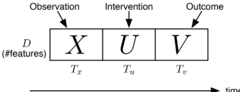
Dynamics-Engineering Problem (Informal): Given theobservation dynamics X2RDTx, find the bestintervention dynamics U 2RDTu_{such that some desired property of theoutcome} dynamics V 2RDTvis optimized.

The problem is illustrated inFig 1. In the figure, we split the dynamics (that correspond to, e.g., a hashtag) into three parts,X,U, andV, where the current time is at the end ofX(i.e., immediately beforeU). The input of the dynamics engineering problem isX, plus the knowl-edge of the historical dynamics behavior (e.g., a model). The output of the problem is the best (recommended) intervention dynamicsU_{, such some properties ofVis optimized. Ideally, we} also want to obtain the projected outcome dynamicsV, i.e., as a result ofU.

Let us revisit our Twitter example mentioned above. Under this context, an example engi-neering problem is as follows: Given the observed numbers of the initiators, propagators, and commentators of a particular hashtag within the past 30 minutes (i.e.,XinFig 1), find the best possible intervention dynamics over the next 30 minutes (i.e.,UinFig 1), e.g., using incentive programs or direct promotions, such that the total readership of the hashtag is maximized in the following hours (i.e.,VinFig 1). Note that in the above problem definition, we assume that only the observation (X) is given, while both the ideal intervention (U_{) and the projected} out-come (V) are to be identified.

Of note, the goal of this work is to find what the best intervention dynamicsU_wouldlook

(e.g., using incentive programs, etc.) is a separate problem that is not covered in the present work.

Score function: To define the dynamics engineering problem formally, we first letY= [UV]2RD×(Tu+Tv)denote the concatenation of the two matricesUandV. For example, if we

Table 1. Summary of notations used in this paper.

Variables

X observation dynamics;X₂RDTx.

U intervention dynamics;U₂RDTu_.

V outcome dynamics;V₂RDTv_.

Y Y¼ ½U VŠ 2RDTy_.

Wik thek-thfilter matrix in thei-th layer;Wk2RDTw.

hik thek-th activation vector in thei-th layer;h_ik2RTþTw1

þ .

D the dynamics dimensionality.

Tx,Tw, etc. the temporal length ofXorW, etc.

σi,βi parameters ofP(X|h) andP(h), respectively.

Ki the number offilters ini-th level.

x,y, etc. vectorization ofXorY, etc. (Eq 1).

hi vector concatenation offh_ikgKi_k¼1:

mx,my, etc. length ofxory, etc.

B,d parameters of the score function (Eq 2).

Ccost,Creward cost / reward parameters (Eqs3and4)

Vref pattern to be matched (Eq 3)

ρ tradeoff parameter (Eqs3and4).

c max-pooling parameter.

S,s max-pooling dummy variables;s= vec(S).

Q,p,A canonical variables of Quadratic Programming

Special matrices and operations

In n-by-nidentity matrix

1m×n n-by-mmatrix with 1 in its elements.

0m×n n-by-mmatrix with 0 in its elements.

Subscripts might be omitted for simplicity.

Specialized convolution inEq 7

Kronecker product

vec() vectorization of a matrix

doi:10.1371/journal.pone.0146490.t001

Fig 1. Illustration of the dynamics engineering problem.X: observation dynamics;U: intervention dynamics;V: outcome dynamics.

haveU ¼ 1₃ 2₄

andV ¼ 5₇ 6₈

, thenY¼ 1₃ 2₄ 5₇ 6₈

. Note that this concatenation

is merely for mathematical convenience:UandVstill differ in their meanings and in the kinds of properties we want their corresponding solutions (U_{andV) to satisfy.}

Moreover, lety= vec(Y) denote its vectorization (i.e., its transformation into a column vec-tor):

y_¼vecðYÞ ¼vecð

yT 1 .. . yT D 2 6 6 4 3 7 7 5Þ ¼

y1 .. . yD 2 6 6 4 3 7 7 5

: ð1Þ

Using the same example above, we havevec 1 2 5 6

3 4 7 8

¼ ½12345678ŠT_{. Accordingly,}

we can reformulate the engineering problem as maximizing ascore functiondefined as:

scoreðy_{Þ ¼}yT_ByþdT_y

: ð2Þ

whereBandddefine the quadratic and linear parts of the score function, respectively. We note that this quadratic score function is general, in the sense that different goals can be achieved using various special cases. In particular, two interesting special cases are:

• Pattern matching: To achieve an ideal outcomeVrefwhile minimizing the cost associated

with the required interventionU, one can maximize the following score function:

scorematchðYÞ ¼ ð1 rÞjjV Vrefjj

2

f rhCcost;Ui

¼ yT_ByþdT_y: ð3Þ

Thefirst term denotesmismatchand will forceVto matchVref; the second term denotescost

and will typically force values inUto be small. Hereρ2[0, 1] controls the relative impor-tance of mismatch versus cost. Moreover,Ccostencodes the relative expense of controlling

different features at different time, whereashU,Ci=∑_{ijUijCijdenotes the dot product}

betweenUandC. For example, suppose_Ccost¼ 1₂ 1₂

andU ¼ 1₃ 2₄

, thenhCcost,Ui

= 1×1 + 1 × 2 + 2 × 3 + 2 × 4 = 17. Returning to our Twitter example above, suppose that the

first row ofU ¼ 1₃ 2₄

represents the numbers of propagators (i.e., one propagator att= 1

and two propagators att= 2) and that the second row represents the numbers of

commenta-tors (i.e., three commentacommenta-tors att= 1 and four att= 2), then assigning_Ccost¼ 1₂ 1₂

is

equivalent to specifying that it is twice as expensive to grow the number of commentators (Twitter users who spend time to leave comments) than to control the number of propaga-tors (who simply click“retweet”), regardless of time. Finally, we note thatEq 3is a special case ofEq 2. To check this, we can rewrite the second line ofEq 3usingB¼ ð1 r_Þ^I T_v^_{I v},

d¼vecð½ r_Cu2_ð1 r_ÞV_refŠÞ, and^_{I v¼ID ð½0}

TvTu ITvŠÞ. Heredenotes the

Kro-necker product (seeTable 1for a summary of notations).

function:

score_profitðYÞ ¼ rhCcost;Ui þ ð1 rÞhCreward;Vi

¼ dT_y; ð4Þ

Thefirst term denotescostand will typically force the values inUto be small; the second term denotesrewardand will typically force the values inVto be large. Similarly to the above task, we useCcostto encode the relative cost and useCrewardto encode the relative reward of

different dimensions and time. Following the above Twitter example, assigning_Creward ¼

1 3 1 3

is equivalent to specifying that it is three times more rewarding to acquire a user

(either a propagator or a commentator) att= 2 compared to acquiring a user att= 1, regard-less of the type of the user. Like the case ofEq 3,ρcontrols the relative importance of cost versus reward. We note thatEq 4is another special case ofEq 2. To check this, we can rewrite the second line ofEq 4usingd¼vecð½ r_{Ccost ð}1 r_{ÞCrewardŠÞ}.

Formal Definition: While maximizing the score function, we make two implicit assump-tions: (1) there exists a temporal dependency amongXandY= [U V], and (2) the solution we come up with needs to follow that dependency. Accordingly, we propose the following formal definition of our problem:

Dynamics-Engineering Problem (Formal): Given observationX, a probabilistic modelP

(), and a score function score(Y), find:

Y¼ ½UVŠ ¼arg max

Y

logPðYjXÞ þlscoreðYÞ: ð5Þ

HereP() denotes the log-likelihood using a probabilistic model that captures the temporal dependencies of the social dynamics. In other words, while the second term (i.e., the score function) takes care of the specific engineering task, thefirst term (i.e., logP(Y|X)) makes sure that the solution still conforms with the temporal dependency of the social dynamics. More-over,λ0 is a balancing parameter that controls the relative importance offitting the proba-bility distributionP() versus maximizing the score. Of note, the selection ofλis crucial and will be described in detail later.

We note that our proposed problem definition isgeneralyetprecise. Indeed, it can incorpo-rate any combination ofP() and score(Y) functions, in which any different combination corre-sponds to a different engineering task. Also, once this combination is given, the engineering problem is mathematically precise.

3.2 Deep-Learning Model

In principle, any probabilistic model of social dynamics can be plugged into the likelihood termP() inEq 5. In this work, we use theRecursive Convolutional Bayesian Model (RCBM)

that we proposed recently [24]. As it will be shown in the experimental section, the choice of this model makes a big difference.

According to RCBM, the basic generation process for dynamicsXis:

Pðh;bÞ ¼ 1

b exp P

kjjhkjj1

b

PðXjh;W;sÞ ¼

ffiffiffi 2

p

s ffiffiffi p

p exp jjX P

kWkhkjj

2

F

2s2

;

More specifically, RCBM assumes that dynamicsX(or more generally, the concatenation of [X U V]) are generated from making“scaled copies”of thefilter matrices Wk’s, where the time

shift and the scaling of these copies are determined by the sparseactivation vectors hk’s. Such a

“scale-and-copy”operation is carried out using the operatorinEq 6, which denotes a dimen-sion-wise convolution defined as:

ðWhÞ½d;tŠ ¼X

Tw

s¼1

h½tþTw sŠ W½d;sŠ 8d;t: ð7Þ

We note that this operator differs from the conventional matrix convolution used in [25,26]. Effectively,doesD1-D convolutions between each row ofWand the entireh, and puts back the results to each row of the output matrix separately.

By stacking multiple levels of the basic form inEq 6, we can construct a deep-learning archi-tecture:

PðX;hÞ ¼ Y

l

PðXljhl;Wl;slÞPðhl;blÞ

¼ 1

Zexp

X

l

jjXl

P

kWl;khl;kjj

2

F

2s2

l

þ

P

kjjhl;kjj1

b_l !

:

ð8Þ

The key of this construction is building the upper-level dynamicsXlbymax-pooling[25,26]

the lower-level activation vectorshl−1,k. This essentially takes the maximum value overc

conse-cutive values of the lower-level activation vectors. This operation introduces non-linearity into the model, which is key for the superior performance of deep-learning methods [24–26].

In [24], we have derived an efficient algorithm for learning RCBM and have demonstrated several applications (i.e., pattern discovery, anomaly detection) inunderstandingsocial dynam-ics. In the present work, we shift focus from understanding toengineeringsocial dynamics.

3.3 RCBM-based Formulation

By writing down the conditional probabilityP(Y|X) using the joint probability specified inEq 8

and then pluggingP(Y|X) into the first term ofEq 5, the optimization problem inEq 5can be explicitly written as:

arg min

Y;h1;h2;S

1 2jj½X YŠ

X

k

W1kh1kjj

2 Fþ s2 1 b1 XK1

k¼1 jjh1kjj1

þ1

2jjMPðh1Þ X

k

W2kh2kjj

2 F þs 2 2 b2 X K2

k¼1

jjh2kjj1 ly

T_{By d}T_y

ð Þ

s:t: h1k0; h2k0andy0:

ð9Þ

Here, a two-level RCBM is presented for illustration purposes, though the optimization formu-lation for a multilevel RCBM can be similarly derived. The max-pooling operation MP() is defined as

MPðh_1Þ½k;tŠ ¼ max

i21;;ch1k½ðt 1ÞcþiŠ; ð10Þ

whereh1is the vector concatenation offhikg Ki

k¼1. As mentioned in Section 3.2, MP() is the key

nonlinear features of the series. However, it also imposes significant difficulties in optimization by making the problem non-differentiable and non-convex. Consequently, the problem inEq 9

is not only difficult to solve, but also prone to getting stuck at suboptimal solutions.

3.4 Convex Relaxation and QP transformation

To solve the difficulty resulted from max-pooling, we propose the following convex relaxation:

arg min

Y;h1k;h2k;S

1 2jj½X YŠ

X

k

W1kh1kjj

2

Fþ

s2 1

b1

X

K1

k¼1 jjh1kjj1

þ1₂jjS X

k

W2kh2kjj

2

Fþ

s2 2

b2

XK2

k¼1 jjh2kjj1

l_ðyT_ByþdT_yÞ

s:t: h1k0; h2k 0andY0;

h1k½ðt 1ÞcþiŠ S½k;tŠ

S½k;tŠ X

c

i¼1

h1k½ðt 1ÞcþiŠ:

ð11Þ

The idea behind this relaxation consists of introducing a new variableSas the surrogate of MP (). Furthermore, we substitute theequalityconstraints specified inEq 10with two sets of

inequalityconstraints, i.e.,

max

i21;...;ch1k½ðt 1ÞcþiŠ S½k;tŠ

Xc

i¼1

h1k½ðt 1ÞcþiŠ:

In other words, instead of forcingSto equateS½k;tŠ ¼ max_i21;...;ch1k½ðt 1ÞcþiŠ, i.e., the

maximal value among the consecutivecvalues, we now constrain it to be larger than or equal to the maximal value, but smaller than or equal to the sum of thosecvalues.

We note that the problem inEq 11is nowjointlyconvex inY,h1,h2andS, since the objec-tive function is convex and all constraints are linear. Moreover, since the objecobjec-tive is differen-tiable, a possible approach to solveEq 11is using the proximal method [27]. It turns out, however, the projection functions corresponding to the constraints inEq 11, which are required in the proximal method, are difficult to derive.

We solve this issue by noting that the objective function ofEq 11is quadratic with only lin-ear constraints. Therefore, in principle, there exists a quadratic programming (QP) transforma-tion that is equivalent toEq 11. The explicit form and the mathematical details of this QP transformation is described inS1 Appendix. We note that, since the problem is jointly convex, QP is guaranteed to find an approximate solution in polynomial time. In our experiments, the QP has around 1000 variables and the problem gets solved in just a few seconds.

3.5 Data-driven evaluation

For the dynamics engineering problem, we argue that the key property of a good solution consists ofcombininga high score and a highvalidity, where the latter can be roughly defined as how well the solution is supported by historical samples that achieve high scores. To show that having a high score alone is not sufficient, consider the case whenλ_{! 1}inEq 5. In this case, the optimization will produce the highest possible score, while completely ignoring the likelihood term inEq 5. As a result, the optimization will produce a solution that does not pos-sess any inherent temporal dependency of the data. In this case, the projected outcomeV would be unlikely to happen in the real world even if the suggested interventionUis implemented.

3.5.1 Validity. As mentioned above, the informal definition of validity is how well the solution is supported by historical samples that achieve high scores. To formally definevalidity

γ, two important components are: (1)_P^_{that denotes the density function capturing what the}

high-scoring dynamics look like in historical data, and (2)q0that denotes a carefully chosen threshold. More precisely,_P^_{ðÞandq0are constructed in four steps:}

1. Evaluate the value of the score function using all historical samplesf½Xi;YiŠgNi¼1, rank them

according to their evaluated values, and then keep only theN0top-scoring samples.

2. Use the first halff½Xi;YiŠgb N₀

2c

i¼1 to construct a kernel density estimator [29]:

^

PðX;Y;hÞ /X

i

expjj½X;YŠ ½Xi;YiŠjj

2

2o2 :

3. Use the second halff½Xi;YiŠgN0 i¼bN0

2cþ1

to choose the value ofωthat has the highest data

likelihood.

4. Use the second half to calculateq0, such that only a small fraction (e.g., 5%) of samples among the second half has_P^_{ðX;Y;hÞ<q0.}

With_P^_{ðÞandq0defined, we can define thevalidityγcorresponding to a solutionY(λ)}

(i.e., solution ofEq 5using a specific value ofλ) as:

gðlÞ ¼ logP^ð½X;Y

_ðlފÞ

q0

: ð12Þ

Then we can useγas a convenient measure, such thatγ0 indicates that, according to histori-cal high-scoring data, the solution is“realistic enough”.

The main idea behind the above procedure is to construct_P^_{ðX;YÞas the density estimator} of the high-scoring historical samples, and then constructq0as thequantile estimator(e.g., at 5%) for the empirical distribution of {Pi}i. HerePi ¼P^ðXi;YiÞdenotes the value ofP^ðÞ

evalu-ated usingXiandYi. Therefore, when the density of a solutionP^ð½X;YðlފÞis larger thanq0 (i.e., whenγ0 inEq 12), we call this solution as being“realistic enough”, because it is more likely (i.e., more realistic) than the 5% most-unlikely high-scoring historical samples.

Consequently, in principle,N0should be selected as a small fraction (e.g, 10%) of the size of the historical samples.

Finally, we note that_P^_{ðX;YÞandq0depend on the partitioning in the second and the third} steps, which, according toEq 12, can also affectγ(λ). A simple way to remove such a depen-dency is to use multiple random partitionings, obtain the corresponding copies of_P^_ðX;YÞ’s andq0’s, and then calculate the average value ofEq 12using all these copies.

3.5.2 Selection ofλ. With validity defined, we are now ready to selectλ. As mentioned before, it should be the combination of high validity and high score. A key observation fromEq 5is that one can make the score larger by makingλlarger. Therefore, while there may be many potential ways to do it, we propose the following method:

arg maxl l

s:t: gðlÞ 0; ð13Þ

where the idea is that conditioned on the solution being (sufficiently) valid, we want its score to be as high as possible. Finally, we use a Twitter dataset to demonstrate the interplay amongλ, validity (γ), and score while engineering social dynamics in the next section.

4 Experimental Results

For experimental results, we first describe our dataset, the overall setup, and two baseline meth-ods. Then, we present experimental results on two engineering tasks: pattern matching and profit maximization.

4.1 Dataset

We use the Twitter dataset from [2] that consists of 181M postings during June to December of 2009 from 40.1M users and 1.4B following relationships. With this dataset, hashtags are used to enumerate the information tokens that carry social dynamics. We filter out“low-traffic” hashtags by selecting only the ones with at least 100 total usages around the 90 minutes during their peak times, yielding a 10K-sample dataset of social dynamics. We then sort these samples according to their peak time. The first 9K samples are used as the training set, i.e., for model training and the construction of_P^_ðÞandq

0(mentioned in Section 3.6), whereas the remaining 1K samples are reserved for testing. This data partitioning scenario ensures that all training data occurs prior to testing data, i.e, no“future data”is used while testing. Finally, for all hash-tag samples, we measure the dynamics in units of 3 minutes, where thefirst 30 minutes are the observation dynamics (X), the middle 30 minutes are the intervention dynamics (U), and the last 30 minutes are the outcome dynamics (V).

We characterize each social dynamic using its five types of users [4].Initiatorsdenote the users who use this keyword before any of his or her friends did.First-time propagatorsand

first-time commentatorsdenote the users who retweet and tweet, respectively, about this key-word after his or her friends using the same keykey-word before.Recurring propagatorsand recur-ring commentatorsdenote the users who retweet and tweet, respectively, the same keyword that they used before. Of note, it means thatX,U,V2R5×10because now each variable has five features and ten timesteps (i.e., three minutes per timestep).

4.2 Setup

intervention cost in time and for different types of users. Similarly, for profit maximization, we setCcost=1D×TuandCreward=1D×TvinEq 4. Of note, the assignment ofVrefinEq 3depends on

the particular experiment and will be detailed later.

In order to analyze the interplay and tradeoffs critical to real-world engineering applica-tions, for each task, we conduct analyses along the following four directions:

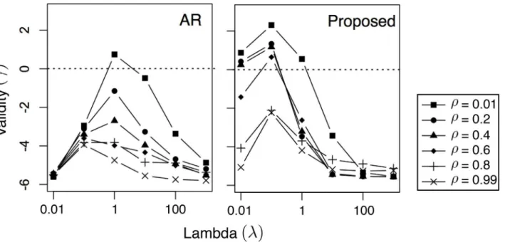
1. Interplay between validityγ(Eq 12) and the optimization parameterλ(Eq 5).

2. Tradeoff of individual terms in the score functions. In particular, for pattern matching (Eq 3), it includes cost (<Ccost,U>) and mismatch (jjV Vrefjj2f); for profit maximization (Eq

4), it includes cost (<Ccost,U>) and reward (<Creward,V>).

3. Comparison between“real”vs. engineered cases. The motivation behind this analysis is to quantify the potential benefits as a result of purposeful engineering, compared to what hap-pened in reality.

4. A case study.

4.3 Baseline Methods

AR: Our first baseline is to substitute the likelihood term inEq 5with another one using the Autoregressive model (AR). AR is commonly used in time-series forecasting and is defined as:

xt¼

X

p

i¼1

Fixt iþt ð14Þ

Herext2RD×1denotes the multivariate features at timet;tNð0; SÞdenotes the i.i.d.

mul-tivariate Gaussian noise;Fi’s denote the matrices for modeling the dependency between the current dynamics and its history back topsteps, where we setp= 10. Details of solvingEq 5

with thefirst term using AR is given inS1 Appendix. While this baselinefits perfectly in our proposed framework, its restrictive linear generative model may limit its performance.

NN: Our second baseline is based on the nearest-neighbor (NN) search. The idea is to search within the training data for the top 5% samples that are the most similar to the given observationX(using Euclidean distance). Then the solutionYis obtained using the {U,V} part of the highest-scoring sample within that subset. The advantage of NN is that, unlike other methods, it doesn’t have a concern about validity, i.e., whether the solution is realistic or not, because the solution is generated from real dynamics that happened in the past. However, its disadvantage is that not all historical dynamics matches the observationXand maximizes the score function at the same time. Consequently, the score of NN’s solution may be low or unstable.

4.4 Experiment 1: Pattern Matching

In our first experiment, i.e., pattern matching, we are given the observationXiof every test

sample and we aim at matching a singleVref. ThisVrefis defined as the average outcome

dynamics of the top 2% samples in the training set with the highest long-term popularity ||V||1. We conduct dynamics engineering using all test samples and analyze the resulting validity, cost, and mismatch.

valid solutions. In particular, that range changes with the value ofρ: the lowerρis, the larger the range is. This is because a lowerρputs more emphasis on minimizing mismatch instead of cost (seeEq 3). While there is nothing unrealistic about the pattern that needs to be matched, matching it using an extremely low cost (i.e., using a largeρ) can be unrealistic. Second, the proposed method outperforms the AR baseline in terms of validity, since the results using the proposed method have a lot more cases above the dotted line (indicatingγ0) compared to AR. This is because the proposed method incorporates RCBM that can effectively capture non-linear features, whereas AR is a non-linear model.

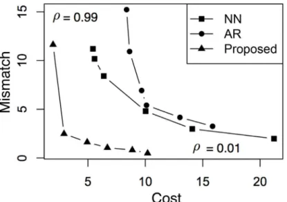
4.4.2 Cost-mismatch Tradeoff. InFig 3, we further analyze the tradeoff of using different values ofρwhereλis selected usingEq 13. In cases when there is noλthat satisfiesγ(λ)0, we select arg maxλγ(λ) instead. The results of average cost versus mismatch using all three

methods are summarized inFig 3. For each method, the point in the lower-right corner corre-sponds to the case ofρ= 0.01, whereas the point in the upper-left corresponds to the case ofρ = 0.99. From the figure, the newly proposed method consistently makes the best tradeoff: with the same mismatch, it achieves a lower cost; with the same cost, it achieves the lower mismatch. The reason for this is twofolds: for AR, its linear model is too restrictive to reach either of the two objectives; for NN, the samples in the subset of training data that matches the given obser-vation does not necessarily have a high score. Another interesting obserobser-vation is that NN seems to make better tradeoffs compared to AR. This shows that the selection of a good genera-tive model is crucial for dynamics engineering.

4.4.3 Constrained Cost Minimization. In order to demonstrate the potential benefits of purposeful engineering, we use a slightly different setting. While for each test samplei, we are still given the observation partXi, we setVref=Vi, i.e, its own outcome dynamics. This setting

allows us to compare the performance of the matching algorithms, in terms of cost, with what actually happened in reality, assuming that each test sample was actually performing a (perfect) matching task without consciously considering minimizing the cost.

Since therealcase achieves a“perfect match”, we need to constrain the engineering algo-rithms such that they can be compared on the same footing. Therefore, we enforce an addi-tional constraint ||V−_{Vref||1pDTvwherep= 5%. In other words, after going through every} test sample, each algorithm will have its own fraction of valid answers, and only the valid answers will be compared to the same set of samples, in terms of cost, to the real case. For AR and the proposed method, a valid answer must satisfy this constrainton top ofsatisfyingγ0.

Fig 4summarizes the results where the fraction of valid answers are annotated at the top and the mean values are marked using red crosses. From the figure, we note that NN produces valid answers for 41% of the test samples, whereas the number is 10% for AR and 98% for the proposed method. Also, the mean cost among the valid solutions using NN is 4.34, compared to 4.82 for AR and 2.31 for the proposed method. In other words, the proposed method achieves not only the largest fraction of valid solutions, but also the lowest average cost for that larger fraction. Note that the cost produced by NN has a high variation, confirming our Fig 3. Tradeoff between cost and mismatch using different values ofρ.For each method, the point in the lower-right corner corresponds to the case ofρ= 0.01, whereas the point in the upper-left corresponds to the case ofρ= 0.99.

doi:10.1371/journal.pone.0146490.g003

Fig 4. Cost distribution of valid answers using different methods.The cost distribution of each method is contrasted with that of the same set of samples in the real case. The mean values are marked using red crosses.

expectation in Section 4.3. Finally, they all achieve lower cost than the corresponding samples in the real case, which is somewhat expected because the real cases were not consciously mini-mizing the cost. This further highlights the cost-saving potential of these dynamics-engineering methods.

4.4.4 Case Study. To gain further insights, we pick a test case where all three methods pro-duce valid solutions from the experiment ofFig 4and plot their suggested solutions inFig 5. For AR and the proposed method, since their solution only cover the last 60 minutes, their first 30 minutes are copied from the real case. From the real case, we see that it is a rather sustained dynamics that seems to be full of interactions among different types of users. To compare among different solutions (i.e., NN, AR, and Proposed), we note that the ideal pattern-match-ing should achieve both low cost durpattern-match-ingt2[30, 60] and low mismatch duringt2[60, 90].

The solution produced by NN, although seems to match the real case in its general shape, it produces a moderate mismatch. Further, the cost of its suggested intervention is the highest among the three. AR, on the other hand, produces a very smooth dynamics that does not match the general shape of (the third part of) the real case, although the mismatch is quantita-tively comparable to that of NN. Moreover, although its cost is relaquantita-tively low, the dynamics doesn’t look real: in fact, its solution validityγis 0.02, i.e., barely passes 0.

Finally, the proposed method produces a recommendation that best matches the third part of the real case, while also producing the lowest-cost intervention. A closer inspection shows

Fig 5. Case study: real versus the suggested dynamics using different methods.A good solution is characterized by low cost (duringt2[30, 60]) and low mismatch (duringt2[60, 90]). The X-axis denotes time (in minutes) and the Y-axis denotes the normalized number of different types of users.

that although the magnitude of the intervention dynamics (i.e., the second part) is generally low, it seems to consciously keep an interesting proportion and interaction among different types of users, i.e., initiators and first-time propagators aroundt= 50, 1st-time commentators aroundt= 55, and recurring commentators aroundt= 65. This shows that the key features for successful dynamics engineering are not necessarily unique and may involve the interaction of multiple features. This is made possible because the proposed recommendation explicitly use the patterns (i.e., the filtersW’s in Eqs9and8) at different temporal scales that are learnt directly from data. Consequently, the proposed method is able to recommend low-cost, good-matching solutions while still making the suggested dynamics follows the intrinsic temporal dependencies from the data.

4.5 Experiment 2: Profit Maximization

In our second experiment, i.e., profit maximization, we are given the observationXiof every

test sample and aim at maximizing the long-term popularity (reward) ||V||1with minimum cost ||U||1. Again, we conduct dynamics engineering using all test samples and analyze the resulting validity, cost, and reward.

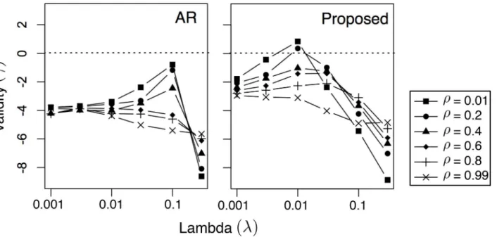
4.5.1 Validity (γ) vs.λ. InFig 6, we present the effects of different values ofλon the aver-age solution validityγ, where the dotted horizontal lines marksγ= 0 (above which the solution is considered valid). There are two observations inFig 6that are consistent withFig 2. First, there is a range ofλthat produces valid solutions; the lowerρis, the easier to produce valid solutions. Since a lowerρputs more emphasis on reward instead of cost (seeEq 4), it suggests that the key to produce good solutions is putting a low (numerical) weight on cost. Second, the proposed method outperforms the AR baseline in terms of validity, indicating that the pro-posed method produces a lot more valid cases (γ0) compared to AR. This confirms that the proposed method incorporates RCBM that can effectively capture non-linear features, whereas AR is a linear model.

Interestingly, there are also three observations inFig 6that are different from that ofFig 2. First, the validity valueγis generally smaller, indicating that as a task, profit maximization is

more challenging than pattern matching. Second, the bestλ’s that correspond to the highestγ’s are also about 10Xsmaller than that ofFig 2. It suggests that in profit maximization, one must put more emphasis on the likelihood instead of the score inEq 5. Finally, the range ofλthat is above zero (λ0.01) is much more narrow than the case ofFig 2(λ2[0.01, 1]). This confirms that the task of profit maximization is more challenging than pattern matching.

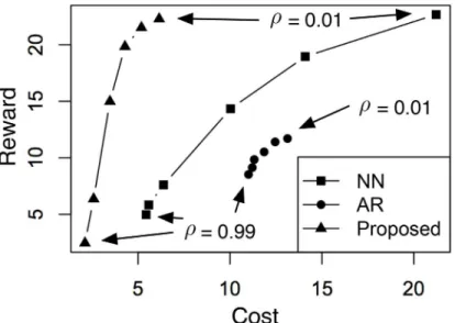
4.5.2 Reward-cost Tradeoff. InFig 7, we further analyze the tradeoff of using different values ofρwhereλis selected usingEq 13. Again, in cases when there’s noλthat satisfiesγ(λ)

0, we select arg maxλγ(λ) instead. The results of average reward versus cost using all three

methods are summarized inFig 7. For each method, the point in the upper-right corner corre-sponds to the case ofρ= 0.01, whereas the point in the lower-left corresponds to the case ofρ= 0.99. We note that, in general, the proposed method provides, again, that best overall tradeoff compared to NN and AR, which confirms that the selection of a good generative model is cru-cial for dynamics engineering. This is also consistent with the observations inFig 3.

Interestingly, there are also two observations inFig 7that are somewhat different from the case ofFig 3. First, while NN seems to be slightly better than AR inFig 3, it is significantly bet-ter in the case ofFig 7. It indicates that, due to the increased difficulty of profit maximization (compared to pattern matching), AR becomes no longer useful. Second, the reward produced by the proposed method is comparable to that of NN, although the proposed method requires much less cost. This suggests that in profit maximization, reducing cost is much easier than increasing reward. This also makes intuitive sense: while it is hard to beat the“Ice Bucket Chal-lenge”in popularity, it might be possible to engineer its marketing campaign such that the cost can be reduced.

4.5.3 Constrained Reward Maximization. To demonstrate the potential benefits of pur-poseful engineering, we now use a slightly different setting. While for each test samplei, we are still given the observation partXi, we enforce an additional constrain that the a solution must

produce a cost that is at mosthalfof theactualcost of samplei, i.e., ||Ui||1, on top of achieving

γ0, to be considered avalidanswer. This setting allows us to compare the performance of the profit-maximization algorithms, in terms of reward and cost, against what actually hap-pened in reality.

Fig 7. Tradeoff between cost and mismatch using different values ofρ.For each method, the point in the

upper-right corner corresponds to the case ofρ= 0.01, whereas the point in the lower-left corresponds to the case ofρ= 0.99.

Fig 8summarizes the results; again, the fraction of valid answers are annotated at the top and the mean values are marked using red crosses. From the figure, we can make three observa-tions. First, the fractions of valid samples are significantly lower than the case ofFig 4. Indeed, NN produces valid answers for 36% of the test samples, whereas the number is 4% for AR and 45% for the proposed method. This confirms that profit maximization is, in some sense, harder than pattern matching. Second, while all valid solutions from each of the three methods have an average cost lower than half of the corresponding real cases (per our experimental design), these methods result in different reward distributions. Indeed, AR, NN, and the proposed method produce lower, comparable, and higher rewards compared to the real cases, respec-tively. This confirms that the proposed approach outperforms the two baseline methods and further highlights the profit-maximization potential of the proposed dynamics-engineering method.

4.5.4 Case Study. To gain further insights, we pick a test case where all three methods pro-duce valid solutions from the experiment ofFig 8and plot their suggested solutions inFig 9. All settings remain the same as the case ofFig 5. To compare among different solutions (i.e., NN, AR, and Proposed), we note that the ideal profit maximization should achieve both low cost duringt2[30, 60] and high reward duringt2[60, 90].

FromFig 8, we can see that, although the solutions from all three methods (NN, AR, and the proposed method) have costs lower than half of the real case, their rewards are quite differ-ent. For NN, the reward of its solution is comparable to that of the real case. Given that it also has a lower cost compared to the real case, this solution is not too bad. For AR, while the reward is even lower, the real issue is that the solution dynamics doesn’t look real: in fact, its solution validityγ0.004, i.e., barely passes 0. Finally, the proposed method not only produces a recommendation that has a low cost, but also a reward higher than the real case. A closer inspection shows that although the magnitude of the intervention dynamics (i.e., the second part) is generally low, it seems to contain interesting interactions because the recommendation Fig 8. Cost distribution of valid answers using different methods.The cost distribution of each method is contrasted with that of the same set of samples in the real case. The mean values are marked using red crosses.

includes different key roles at different stages: recurring commentators (red) around time

t= 35, first-time propagators (dark blue) aroundt= 50, and then the dominating first-time propagators aftert60. All these interactions reflect the patterns (i.e., the filtersW’s in Eqs9

and8) of different temporal scales that are learnt directly from data. This is why the proposed method is able to recommend solutions with low cost and high reward, while still making the suggested dynamics follow the intrinsic temporal dependencies from the data.

5 Discussion

5.1 Pattern Matching vs. Profit Maximization

The merits of the proposed pattern matching and profit maximization are quite different. Indeed, fromFig 4, the proposed pattern matching is capable of producing valid solutions for 98% of the test samples, while reducing the cost by an average of 82% with a minor mismatch within 5%. On the other hand, fromFig 8, the proposed profit minimization is capable of pro-ducing valid solutions for 45% of the test samples while improving the reward by an average of 27% with less than half of the original cost. Such a difference originates from the two tasks’ dif-ferent goals and formulations: pattern matching (Eq 3) aims at matching a given pattern with the lowest cost, whereas profit maximization aggressively maximizes reward and minimizes cost.

Fig 9. Case study: real versus the suggested dynamics using different methods.A good solution is characterized by low cost (duringt₂[30, 60]) and high reward (duringt₂[60, 90]). The X-axis denotes time (in minutes) and the Y-axis denotes the normalized number of different types of users.

Further, such a difference in formulation implies a difference in the fundamentaldifficulties

of two tasks. More importantly, profit maximization is significantly more difficult because while the“cost”has a natural lower bound (i.e., zero), the“reward”, in principle, does not have any upper bound. In other words, unless the parameterλis assigned perfectly, it is very easy to either obtain an invalid solution or a low-score solution. Therefore, in many engineering cases (e.g., marketing promotion), although profit maximization may be more desirable, in practice, pattern matching may be more useful.

The above analysis is confirmed by our experimental results in two ways. First, by compar-ingFig 2withFig 6, we see that it is significantly harder to generate a valid solution in profit maximization. Indeed, compared to the case of pattern matching (Fig 2), the area above the horizontal lineγ0 is much smaller in the case of profit maximization (Fig 6). Also, compared to the case of pattern matching, the range ofλthat corresponds toγ0 (λ0.01) is much more narrow than the case ofFig 2(λ2[0.01, 1]). It suggests that it is harder to select a good value for the parameterλin the case of profit maximization. Second, by comparingFig 3with

Fig 7, we see that while pattern matching is capable of reducing both cost and mismatch, profit maximization is more capable of achieving a reasonable reward using low cost, compared to achieving a very high reward using moderate cost. Indeed, fromFig 7, we see that although the cost of the proposed solution is much lower than the case of the NN (i.e., nearest-neighbor) baseline, their highest possible rewards are only comparable.

These differences among the two tasks have practical implications on their real applications. First, if the ideal outcome pattern is given, pattern matching is the better option because according toFig 4, there is a 98% chance that a valid solution will be produced with low cost and mismatch. Second, if the ideal pattern is not given, then according toFig 8, there is a 45% chance that a valid solution will be produced. In this case, a moderately high reward with a low cost can be expected.

5.2 Future Directions

We believe this work is only the first step toward a new field with great potential, namely, data-driven dynamics engineering. While significant follow-up work can be built on the foundation this work offers, we would like to point out three directions that seem to hold the most prom-ise. The first direction involves exploring different combinations of generative models and score functions as mentioned inEq 5. Although we derive our solution based on a particular model (RCBM) and evaluate it using two specific score functions (Eqs3and4), other combina-tions can introduce equally, if not more, important engineering applicacombina-tions.

The second direction involves building a complete tool chain of dynamics engineering. In that sense, this work only accomplishes the very first component, i.e., figuring out what the ideal intervention should be. Two other important components in the tool chain are (1) how to

implementthat intervention most effectively and most efficiently and (2) how to efficiently val-idatethe effectiveness of intervention given limited resources (i.e., using field experiments).

We note that this work serves as the foundation for the other two components by providing a principled, data-driven method to offer an ideal intervention and its anticipated outcome. Using such information, the engineer gets to eliminate the need for trial-and-error among all possible interventions. Instead, he or she can focus on the implementation and validation per-spectives of dynamics engineering, both of which justify an in-depth investigation on their own right. If we look back at the trajectory of how the tool chain of the Integrated-Circuit industry (worth $300B as of 2016) was built, we are right at the very beginning of it.

mobile context-aware computing, computational economics, and healthcare could potentially also use this framework to engineer their own dynamics problems. In this sense, we believe that developing a discipline for data-driven dynamics engineering is full of potential.

6 Conclusion

In this paper, we have defined a new problem that is full of long-term potential, i.e., the data-driven engineering of social dynamics. To the best of our knowledge, this work brings the fol-lowing new contributions:

1. Data-Driven Dynamics Engineering: We propose a framework for data-driven dynamics engineering. Our formulation is precise yet general and includes pattern matching and profit maximization as special cases. Using a deep-learning model, we derive a solution based on convex relaxation and quadratic-programming transformation, which is efficient with guaranteed global convergence. We also propose a data-driven evaluation method instead of the time-consuming and expensive field experiments [17].

2. Pattern Matching vs. Profit Maximization: Using a Twitter dataset, the proposed pattern matching generates valid solutions in 98% of the test cases, achieving an average cost reduc-tion of 82% with a mismatch within 5%. Moreover, the proposed profit maximizareduc-tion gen-erates valid solutions in 44% of the cases, achieving an average reward improvement of 27% with a cost reduction of at least 50%. We further report and analyze the interesting tradeoffs in how to chose among these two tasks, as well as the factors that are critical to real-world dynamics engineering applications, including solution validity, pattern mismatch, interven-tion cost, and outcome popularity.

Since the proposed formulation applies generally to any multi-dimensional time series, we believe this approach can be also applied to the engineering tasks of other applications. We hope this work serve as the first step in this new field of great potential.

Supporting Information

S1 Appendix. Proof of Theorem 1 and 2; derivation of the baseline solution based on the autoregressive (AR) model.

(PDF)

Author Contributions

Conceived and designed the experiments: HP HL JP RM. Performed the experiments: HP. Analyzed the data: HP HL. Contributed reagents/materials/analysis tools: HP HL. Wrote the paper: HP HL JP RM.

References

1. Naaman M, Becker H, Gravano L. Hip and trendy: Characterizing emerging trends on twitter. Journal of American Society of Information Science and Technology. 2011;. doi:10.1002/asi.21489

2. Yang, J, Leskovec, J. Patterns of temporal variation in online media. Proceedings of WSDM. 2011;.

3. Lehmann J, Gonçalves B. Dynamic classes of collective attention in twitter. Proceedings of WWW. 2012;Available from:http://dl.acm.org/citation.cfm?id = 2187871.

4. Peng HK, Marculescu R. ASH: Scalable Mining of Collective Behaviors in Social Media using Riemann-ian Geometry. In: ASE International Conference on Social Computing; 2014.

6. Chen W, Yuan Y, Zhang L. Scalable Influence Maximization in Social Networks under the Linear Threshold Model. Proceedings of ICDM. 2010 Dec;Available from:http://ieeexplore.ieee.org/lpdocs/ epic03/wrapper.htm?arnumber = 5693962.

7. Barabasi A. The origin of bursts and heavy tails in human dynamics. Nature. 2005;Available from: http://www.nature.com/nature/journal/v435/n7039/abs/nature03459.html. doi:10.1038/nature03459

8. Tsur O, Rappoport A. What’s in a Hashtag? Content based Prediction of the Spread of Ideas in Micro-blogging Communities. Proceedings of WSDM. 2012;.

9. Szabo G, Huberman BA. Predicting the popularity of online content. Communications of the ACM. 2010;.

10. Radinsky K, Svore K, Dumais S, Teevan J, Bocharov A, Horvitz E. Modeling and predicting behavioral dynamics on the web. In: Proceedings of WWW. New York, New York, USA: ACM Press; 2012.

11. Yang J, Counts S. Predicting the Speed, Scale, and Range of Information Diffusion in Twitter. In: Pro-ceedings of ICWSM; 2010.

12. Gupta M, Gao J, Zhai C, Han J. Predicting future popularity trend of events in microblogging platforms. Proceedings of the American Society for Information Science and Technology. 2012;Available from: http://onlinelibrary.wiley.com/doi/10.1002/meet.14504901207/full.

13. Matsubara Y, Sakurai Y, Prakash B. Rise and fall patterns of information diffusion: model and implica-tions. Proceedings of KDD. 2012;Available from:http://dl.acm.org/citation.cfm?id = 2339537.

14. Jansen B, Zhang M. Twitter power: Tweets as electronic word of mouth. Journal of American Society of Information Science and Technology. 2009;Available from:http://onlinelibrary.wiley.com/doi/10.1002/ asi.21149/full. doi:10.1002/asi.21149

15. Romero D, Meeder B, Kleinberg J. Differences in the mechanics of information diffusion across topics: Idioms, political hashtags, and complex contagion on Twitter. In: Proceedings of WWW; 2011.

16. Click, A. Iran’s Protests: Why Twitter Is the Medium of the Movement. Time. 2009 June;.

17. Gerber AS, Green DP. Field experiments: Design, analysis, and interpretation. WW Norton; 2012.

18. Lin Y, Margolin D, Keegan B. # Bigbirds Never Die: Understanding Social Dynamics of Emergent Hash-tag. Proceedings of ICWSM. 2013;Available from:http://arxiv.org/abs/1303.7144.

19. Dow P, Adamic L, Friggeri A. The Anatomy of Large Facebook Cascades. Proceedings of ICWSM. 2013;Available from:http://friggeri.net/bibliography/papers/Dow2013vf.pdf.

20. Asur S, Huberman BA, Szabo G, Wang C. Trends in social media: Persistence and decay. In: Proceed-ings of ICWSM; 2011.

21. Leskovec J, Kleinberg J, Faloutsos C. Graphs over Time: Densification Laws, Shrinking Diameters and Possible Explanations. In: Proceedings of KDD; 2005.

22. Lin Y, Chi Y, Zhu S. Facetnet: a framework for analyzing communities and their evolutions in dynamic networks. Proceedings of WWW. 2008;Available from:http://dl.acm.org/citation.cfm?id = 1367590.

23. Peng HK, Marculescu R. Identifying Dynamics and Collective Behaviors in Microblogging Traces. In: Proceedings of ASONAM; 2013.

24. Peng HK, Marculescu R. Multi-scale Compositionality: Identifying the Compositional Structures of Social Dynamics Using Deep Learning. PloS One. 2015;. doi:10.1371/journal.pone.0118309 25830775

25. Lee H, Grosse R, Ranganath R, Ng A. Convolutional deep belief networks for scalable unsupervised learning of hierarchical representations. International Conference on Machine Learning (ICML). 2009; p. 1–8. Available from:http://portal.acm.org/citation.cfm?doid = 1553374.1553453 http://dl.acm.org/ citation.cfm?id = 1553453.

26. Kavukcuoglu K, Sermanet P. Learning convolutional feature hierarchies for visual recognition. Advances in Neural Information Processing (NIPS). 2010;(1: ):1–9. Available from:http://papers.nips. cc/paper/4133-learning-convolutional-feature-hierarchies-for-visual-recognition.

27. Boyd SP, Vandenberghe L. Convex Optimization. Cambridge University Press; 2004.

28. Wasserman L. All of statistics: a concise course in statistical inference. Springer; 2004.