ABSTRACT: This article presents a retirement analysis model for aircraft leets. By employing a greedy algorithm, the presented solution is capable of identifying individually weak assets in a leet of aircraft with inhomogeneous historical utilization. The model forecasts future retirement scenarios employing user-deined decision periods, informed by a cost function, a utility function and demographic inputs to the model. The model satisies irst-order necessary conditions and uses cost minimization, utility maximization or a combination of the 2 as the objective function. This study creates a methodology for applying a greedy algorithm to a military leet retirement scenario and then uses the United States Air Force A-10 Thunderbolt II leet for model validation. It is shown that this methodology provides leet managers with valid retirement options and shows that early retirement decisions substantially impact future leet cost and utility.
KEYWORDS: Aircraft retirement, Fleet manager, Aircraft cost, Retirement model.
Application of a Greedy Algorithm to
Military Aircraft Fleet Retirements
Jeffrey Newcamp1, Wim Verhagen1, Heiko Udluft1, Richard Curran1INTRODUCTION
Military aircrat leet managers are responsible for providing strategic capability to their owning command. hus, aircrat are based around the globe to perform various roles under a variety of operating conditions. As these individual aircrat are lown over time, each one develops a historical utilization proile that is related to its fatigue life expended (Molent et al. 2012). When a leet of individual assets nears projected end-of-life, it is imperative that the leet manager plan for retirement so that operational demand can be satisied. Retirement planning varies greatly across military services and within service leets (Garcia 2001; AFSB 2011). It can be proactive and data-driven but at times it has been reactionary, data-driven by changing budgetary conditions or critical aircrat failures. As the average age of aircrat leets is increasing, retirement planning tools and methodology are necessary to aid leet managers through the retirement decision process (Carpenter and White 2001).
he objective of this research was to develop a tool to provide leet managers with a list of aircrat serial numbers that should be considered for retirement, sorted by precedence and timing. his tool is called the Fleet and Aircrat Retirement Model (FARM). It provides a list of aircrat indicating which one should be retired irst and when this should happen. To improve the applicability of the tool, its interface is simplistic, the greedy algorithm implementation is clear and the inputs are accepted in a variety of formats. FARM was built for the spectrum of leet managers including those who seek to minimize lifecycle cost, to maximize aircrat utility and to maximize the leet’s utility to cost ratio. he methodology also supports a leet manager who wishes to use his own objective function that might be based on a variety of weighted metrics.
1.Delft University of Technology – Faculty of Aerospace Engineering – Air Transport and Operations Section – Delft/South Holland – Netherlands.
Author for correspondence: Jeffrey Newcamp | Delft University of Technology – Faculty of Aerospace Engineering – Air Transport and Operations Section | Kluyverweg 1 | 2629 HS – Delft/South Holland – Netherlands | Email: [email protected]
Prior to discussing retirement, a fleet manager must understand the fleet’s demands and historical utilization (Jin and Kite-Powell 2000). A previous study analyzed this opportunity using operational data from the United States Air Force (USAF) A-10 hunderbolt II leet (Newcamp 2016). he next step in retirement thinking is to develop replacement policy for a leet utilizing the operation research methodologies contained in the study of replacement theory (Peters 1956). Unfortunately, current leet retirement schemes are primarily based, ater an initial objective screening, on subjective means because economic life calculations are exceedingly complex (Tang 2013; Lincoln and Melliere 1999; Unger 2008). For example, the USAF gathers maintenance and logistics experts to decide which aircrat can get retired; however, the decision is very complex, and the decision-makers lack suitable tools (Marx 2016). Aircrat can be identiied for retirement based on light hours, repairs that limit usability, limit exceedances, corrosion, owning unit capabilities, among many other factors. While the bulk of replacement theory literature discusses the replacement of current (defender) assets with more modern (challenger) assets, this study ignores the latter because their acquisition does not directly hasten defender retirements (Robbert et al. 2013). Also, the authors treat military aircrat as parallel assets that independently contribute to supply (Stuivenberg et al. 2013), which allows for the speciicity of individual serial numbers in the leet.
Military aircrat leet’s assets do not continually operate at maximum capacity. Since retirement schedules depend on utilization, a leet manager may alter utilization patterns leading to a more optimal retirement schedule. Testing various retirement schedules with an objective tool is necessary to quantify the net present value of each scheme. This paper contributes with a methodology that answers this need and enables leet managers to make utilization decisions now that will afect future leet statuses.
The novel contribution of the FARM methodology is the use of individual serial number utilization histories and cost data as a basis for future year predictions. Traditional replacement models have used leet-wide utilization averaging or ignored asset utilization altogether, which has led to non-optimal solutions (Hartman 1999). To overcome the limitation of basing forecasts on outdated information, leet managers can periodically use FARM to update their leet retirement forecasts, including updated cost and utility data for each iteration. his approach also allows leet managers
to alter their utilization levels across a leet to optimize their retirement scheduling.
he remainder of this article will discuss the methodology employed in the FARM software. The background section contains relevant literature on asset retirement plus a discussion of capital asset replacement theory. In the methodology section, the greedy algorithm approach to the retirement problem and the mathematical formulation for FARM are described. hen the results section shows data from a simulation run using FARM for a virtual leet. he discussion section highlights the usefulness of a serial number speciic retirement tool and shows validation of FARM using the real USAF A-10 leet. Lastly, the conclusions section emphasizes the major indings from this study.
BACKGROUND
LITERATURE REVIEWA military aircrat leet retirement methodology must connect the domains of replacement theory, capital asset economics and military operational analysis. Relevant studies concerning asset replacement include Jones et al. (1991), Rajagopalan (1998) and Bethuyne (1998) and the thorough treatment of capital equipment replacement in Jardine and Tsang (2013). While insights can be gained from other domains, 2 considerations are important to aircraft replacements. First, aircrat lifecycles and planning/construction timelines are much greater than some other asset categories. Second, upgrades and overhauls signiicantly alter the capability and lifetime projection (Tang 2013).
Jin and Kite-Powell (2000) relied on system utilization and replacement decisions to meet the demands of a proit-maximizing manager. he authors looked at operating cost trends and the cost of replacement as factors for the retirement decision for ships. he primary contribution of Jin and Kite-Powell (2000) is the conclusion that an asset should be retired if its net beneit in a leet is less than the salvage value.
Evans (1989) studied ship replacement theory basing his approach on costs rather than profits and concluding that replacement should occur when it becomes cheaper to purchase a replacement than to continue operating an aging system. he paper has many similarities to aircrat leet replacement study, mainly that replacement should only be afected by costs in real terms. Additionally, this author posited that replacement decisions should focus on the existing leet and not on the costs or capabilities of the replacement assets. he present study uses the same approach, suggesting that retirement is based on the current operating costs of the leet. Since ship replacement requires years for contracting, construction and testing, ships are more similar to aircrat than assets in the motor vehicle, farm machinery and locomotive industries. As Evans posited, ships are oten replaced with like replacements. However, aircrat are commonly replaced with newer assets with greater capability (Boness and Schwartz 1969).
Malcomson (1979) determined replacement rules for capital equipment and concluded that an iterative approach was the most eicient. Like in this paper, Malcomson also assumed that the replacement trigger point must be when the operating cost of aging assets is greater than operating new equipment. Further, the author noted that inite answers to the replacement problem are more desirable than approximate answers, and given modern computing power, inite solutions are attainable at very low cost.
Landry (2000) analyzed multiple courses of action for maintaining the aging leet of Canadian CF188 (F-18) and CP140 (P-3) aircrat. His study treated the problem as a business case analysis with the aim of providing a leet manager with objective data for a retirement decision. His Airframe Life Extension Program (ALEX) sotware used fatigue test control point data to forecast early retirement dates.
Lu and Anderson-Cook (2015) concluded that future reliability estimations can be improved when assets of the same age are not treated homogeneously, but are rather based on historical usage. he authors used an automobile example to illustrate that 2 cars of the same age do not possess the
same reliability. Understanding mileage and usage conditions can improve maintenance and replacement decisions, just as understanding aircrat demographics can improve retirement decisions.
REPLACEMENT THEORY
Replacement theory is a decision-making process from operations research dealing with substitute system selection conducted by an agent. For a group of assets, the formulation becomes a parallel replacement problem. If the goal is to minimize lifecycle cost, replacement theory can help to determine a capital asset’s optimum life. As capital assets age, increasing maintenance costs and reduced utility draw attention to the necessity for replacement (Bethuyne 1998; Lu and Anderson-Cook 2015). Retiring assets is half of the parallel replacement puzzle and the subject of this research. It is assumed that the selection of replacement equipment occurs outside the scope of this methodology.
Generally, new equipment with better capability replaces older equipment (Nair and Hopp 1992). For aircrat, replacement theory might suggest 2 courses of action: upgrades/overhauls or retirement. As Landry’s research concluded, the crux is deciding whether it is more fiscally responsible to upgrade aircraft structure or to replace the aircrat altogether (Landry 2000). his paper only addresses the retirement course of action, which is termed the replacement model. It is believed that providing a leet manager with the best replacement model will yield the most sensible economic replacement policy.
A parallel replacement problem, by its nature, addresses a set of assets. Unlike the single asset case, assets under consideration for parallel replacement can have their utilization levels adjusted to prolong or accelerate deterioration (Bethuyne 1998). his can be an invaluable approach for leet managers trying to meet operational requirements or retirement mandates.
METHODOLOGY
FRAMING THE PROBLEMsince a greedy algorithm provides the same global optimum if the problem is appropriately bounded and local optima are avoided through logic (Cormen et al. 2009). h is model consisted of a l eet of n aircrat with each subsequent l eet size, n − 1, dependent on the previous reduction. h is methodology
was grounded in the assumption that a l eet manager desiring to retire 2 or more aircrat would always choose the worst asset to retire at each iteration. h erefore, all smaller l eet size problems became n – 1 easier until n − (n − 1), when the single remaining aircrat was the least desirable option. h is iterative approach resulted in a Pareto front of l eet cost, l eet utility or the ratio of l eet utility to cost. Changing from a minimization model to a maximization model, a second Pareto front could be found. h e space between the Pareto fronts indicates the relative goodness or inferiority of retirement choices.
FLEET AND AIRCRAFT RETIREMENT MODEL FARM uses a greedy algorithm to determine which aircrat in an inhomogeneous l eet should be retired and in what order. For each smaller l eet size, the algorithm chooses the current optimal solution before analyzing the next smaller l eet size. FARM’s methodology is outlined in Fig. 1. h e multi-year outlook makes retirement decisions using projected asset cost and utility. h e model is valid for any initial and i nal l eet sizes. FARM operates with user inputs (decision periods, minimum/ maximum aircrat ages and rate of yearly budget increase) and 3 user functions (i xed cost, variable cost and utility). h e i xed cost is distributed evenly across assets while the variable cost and utility are both functions of aircrat age. Costs are modeled as equivalent costflow. Inflation and the effects of various
methods for cost reporting were removed from the model by using maintenance man-hours as a proxy in the variable cost calculations. Utility is analogous to aircrat availability, is a number between 0 and 1 and is computed as the number of available days out of 31. However, individual FARM users may alter the format of input functions as necessary.
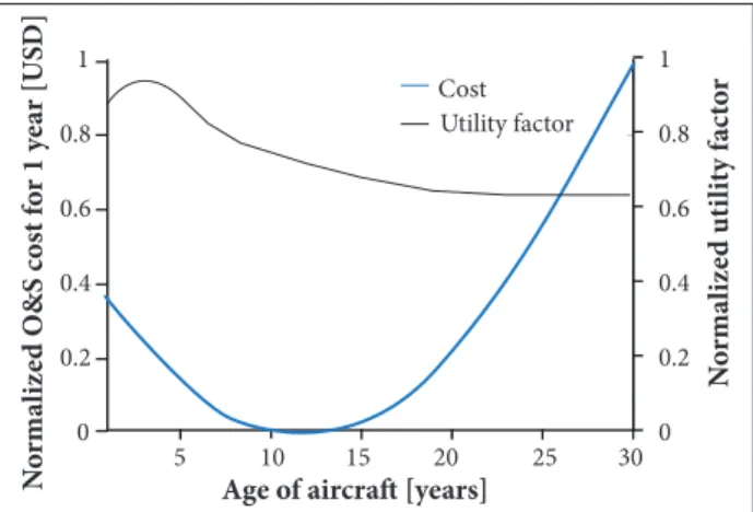
h e methodology underlying FARM is useful for modeling a real l eet of aircrat as well as a virtual l eet of aircrat . Virtual l eet modeling follows the conventions found in literature: aircrat operations and support (O&S) costs are high in the i rst few years of operation, then decrease sharply as the l eet matures and i nally the costs increase at approximately 3% per year of age into the future (Dixon and Project Air Force (U.S.) 2006). Utility begins low for a new aircrat , then quickly peaks, followed by a decrease with age. An example of the cost and utility models used for FARM’s development are shown in Fig. 2. Step functions in utility levels and costs that occur due
Figure 1. Flow chart for methodology steps.
Process candidates for review Cost, utility,
fleet Fleet manager
inputs
Yes
No Greedy algorithm for fleet options Software functions
Calculate current fleet utility Calculate current
fleet cost
Evaluate for forecast periods
Iteration Comparison
Old versus new fleet
configuration New fleet utility
New fleet cost Cost feedback loop
Does new fleet meet budget?
Proccess candidates for review
Does new fleet
improve utility? Store viable solution Store undesirable
solution Yes
No
Figure 2. Representation of cost and utility models in FARM.
Age of aircraft [years] 0 .2
0
5 1 0 1 5 2 0 2 5 3 0
0 .4 0 .6 0 .8 1
N
o
rma
liz
ed O&S c
os
t f
o
r 1 y
ea
r [US
D]
N
o
rma
liz
ed u
ti
li
ty f
ac
to
r
0 0 .2 0 .4 0 .6 0 .8 1 Cost
to major overhaul or repairs were not added to the model. Real l eets were modeled with actual cost and utility functions, which in general were found to follow the published conventions. To forecast future l eet conditions, the most recent cost and utility were extrapolated through time. Otherwise, depending on the age distribution of the l eet, FARM would suggest retiring very young aircrat with high cost and low utility.
For each decision period, FARM outputs the recommended serial numbers to retain for all l eet size options with associated metrics for each option. Fleet managers may use these data to identify their ideal l eet size and makeup. Fleet changes with time can then be evaluated. h e limitations of this methodology and associated software model are few but important. The methodology is only valid for 1 mission design series. For example, a mixed l eet of KC-135s and F-15s cannot be evaluated. Second, the methodology does not allow for subjective valuations or weighting factors for the aircrat . Lastly, FARM does not provide a time-sequence of retirement decisions. Rather, FARM forecasts future asset cost and utility to support a retirement decision forecast.
MATHEMATICAL FORMULATION
This section presents the optimization model that the greedy algorithm solves in each of its iterations for a given year of interest. Lastly, the calculation equations and problem constraints are presented.
h e decision variables are:
The objective function contains 3 terms. The first is the cost calculation, a combination of all fixed and variable costs for operations and sustainment. The second term is the utility calculation, measured as wished by the fleet manager. The third term is the utility per cost ratio, a way to balance the cost associated with changes to utility. It is assumed that only 1 term can be optimized at a time in the model. That is, 1 and only 1 of the weights is equal to 1 each time the optimization model is solved, as shown in Eq. 2. The following equations are required to evaluate the objective function.
h e cost of an aircrat a in year t is the integration of aircrat cost from simulation start until the year of interest, assuming that the integration increment is small enough to yield small error (Eq. 3):
h e objective function (Eq. 1) seeks to maximize:
where:
(1)
(2)
(3)
(4)
(5)
(6)
(7)
where C
a is the annualized cost function of aircrat a. h e utility of an aircrat a in year t is the integration of aircrat utility from simulation start until the year of interest, assuming that the integration increment is small enough to yield small error (Eq. 4):
where U
a is the annualized utility function of aircrat a. h e equations are subjected to several constraints. h e sum of aircrat a in year t must be between the bounds of operational aircrat in year t (Eq. 5):
where N A
t is the minimum number of operational aircrat in year t; A represents the aircrat type, a; N A
t is the maximum number of operational aircrat in year t.
h e sum of the cost of aircrat a times inventory must be less than or equal to budget in year t (Eq. 6):
where B
t is the maximum budget in year t .
h e sum of utility of aircrat a times inventory must be greater than or equal to the minimum acceptable utility threshold in year t (Eq. 7):
where U
t represents the minimum utility threshold of the l eet in year t.
a represents the aircrat of interest; t means year of interest;
C
t ais the cost of aircrat a in year t; X i
t a means that aircrat a is operating in year t in iteration i; W
c, Wu, Wr represent weighting — cost, utility, and utility/cost ratio, respectively; U
h e opportunity to retire an aircrat a in year t is contingent upon the existence of aircrat a in the l eet in the previous year (Eq. 8):
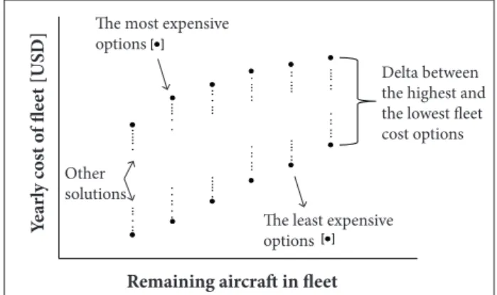
represent the feasible solutions, which include only those results meeting budget and utility requirements. h e bottom curve represents the cost-minimization solutions. h ese solutions show the cost of the l eet for n aircrat , n – 1 aircrat , etc. h e top curve shows l eet cost for cost maximization or worst case retirement choices made for each l eet size. h e vertical gap between the curves is the cost delta that can be saved by making the cost-minimization serial number retirement decisions. h e curves are cutof at the both ends, caused by budget and utility constraints.
Figure 4 is an expanded view of a small portion of the lines in Fig. 3. h is expanded view shows that the lines in Fig. 3 are composed of many discreet points. At each l eet size, n, FARM calculates all of the possible options. h ese are shown in Fig. 4 between the most expensive and the least expensive options. Knowing the range of options is useful because it is not always practical for a l eet manager to retire the optimum aircrat .
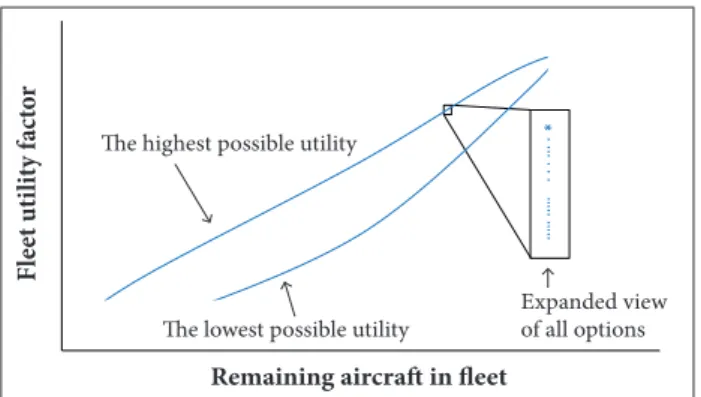
Figure 5 shows the simplii ed simulation results for the same scenario, but with a utility-centered management focus.
(8)
(9)
(10)
(11)
(12)
(13)
where Ri
ta means that the aircrat a is retired in year t in iteration i. h e presence of an aircrat a in year t, given the knowledge of previous years of interest and the decision made in year t, is represented in Eq. 9:
where, upon initialization, all aircrat are operational (Eq. 10):
h e l eet size in year t, Eq. 11, is the summation of the operating aircrat :
where F i
ta is the l eet size in year t in iteration i and must be 1 smaller at each iteration (Eq. 12):
and the initial l eet size, Eq. 13, is the summation of the operating aircrat in the initial year:
RESULTS
h is section presents results from the FARM program. A virtual l eet is used for simulation and simplii ed output plots show representative results. h en, to validate the methodology, A-10 case study FARM results are shown with plots showing detail to the tail number level.
To evaluate FARM, this discussion uses a simulated aircrat l eet of size, n = 100, over a period of 5 years with cost and utility data similar to those represented in Fig. 2. Aircrat ages were drawn from a uniform distribution. Budget was set at the current budget plus a 1% yearly budget increase to mimic the defense budgeting process. Minimum acceptable utility was set to 45% of the existing utility. h ree objective functions are used: cost minimization, utility maximization and utility per cost maximization.
Figure 3 shows simplified simulation cost results for a sample l eet in year 5 for l eet size options from 1:n. h e 2 lines
Figure 3. High and low cost choices for l eet of various l eet
size options.
Fi gure 4. Expanded view of cost options showing all solutions.
Remaining aircraft in fleet
Y
ea
rly c
os
t o
f fl
ee
t [US
D]
Other solutions
The most expensive options
Delta between the highest and the lowest fleet cost options
The least expensive options
The highest possible cost
The lowest possible cost
Remaining aircraft in fleet
Y
ea
rly c
os
t o
f fl
ee
t [US
h ese results inform the l eet manager which serial numbers to retire if the l eet goal was to maximize the utility factor, which for this scenario is the sum of aircrat days available per month for the existing l eet. h e expanded view shows that, for each l eet size, there are n – 1 utility outcomes. h e shapes of the curves shown in Fig. 3 to Fig. 5 are the manifestation of the cost and utility input data.
h e curves in Fig. 6 show the Pareto fronts for the utility per cost ratio calculations for the sample l eet. As aircrat are retired from the l eet (right to let ), the curves diverge, showing that a l eet manager can make poor retirement decisions that impact the l eet’s utility per cost ratio. As the l eet size shrinks, the shape of the Pareto curves shit s which is due to the i xed cost distribution function. Maintaining a constant i xed cost distribution function but varying the l eet retirement scenarios always results in local maxima (optimality condition). h is result is valuable to l eet managers because it recommends a minimum practical l eet sizing solution. For example, this simulation shows a maximum utility per cost ratio that can be achieved for a l eet size of 30 aircrat .
A-10 CASE STUDY
A realistic retirement scenario for the USAF A-10 l eet (2016 active l eet) sought to reduce the l eet size to simulate the closure of a base. Right-censored A-10 data were provided by the USAF and were used as demographic data for FARM. Maintenance man-hour data were provided for each active tail number for each month for i scal years 1995 to 2015 (66,172 total observations). Figure 7 shows 2 dif erent percentile categories for the distribution of man-hours and the median line of the aircrat in the set. For example, the median number of maintenance man-hours for a 14 year-old A-10 was approximately 100 h per month. h e dashed line is a 3% growth prediction, which validates the relationship between aircrat age and maintenance burden for agile aircrat investigated by Dixon and the Project Air Force (U.S.) (2006). The A-10 maintenance man-hour data increased at a rate of approximately 3% per year. A 1-way ANOVA coni rmed this age ef ect (factor: aircrat age; dependent variable: maintenance man-hours; p-factor = 0.014). A 159 USD labor cost rate derived from USAF depot cost data was applied to the man-hour data for illustrative purposes in the case study. Fixed cost and variable cost values were derived from the USAF’s Total Ownership Cost Tool (Robbert et al. 2013).
h e USAF also provided mission capable rates as a utility measure for use in FARM simulations. h ese data were recorded monthly for each active tail number for the years 2009 – 2015 (2,792 observations). h e mission capable rate was a reasonable utility metric to use for the A-10 because it is a function of failure frequency, which represents asset reliability (Balaban et al. 2000). h e mission capable rate data did l uctuate in response to funding changes, upgrades and operational conditions. During the data collection period, for example, the A-10 l eet underwent a system life extension program that altered the
Figure 5. High and low utility choices for various l eet size
options with expanded view of all possibilities.
F
le
e
t u
ti
li
ty f
ac
to
r
Remaining aircraft in fleet
The highest possible utility
The lowest possible utility
Expanded view of all options
U
ti
li
t
y p
er c
os
t r
at
io
[mo
n
ths o
f
ava
il
ab
ili
ty/mi
lli
o
n US
D]
Remaining aircraft in fleet
Maximum utility per cost Minimum utility per cost
0 1. 2 1. 4 1. 6 1. 8 2 2. 2 2. 4 2. 6 2. 8 3
10 20 30 40 50 60 70 80 90
14 0 200 400 600 800 1, 000 1, 200
16 18 20 22 24 26 28 30
25 – 75% range 5 – 95% range
Median
3% growth prediction
Age of aircraft [years]
M
ai
n
ten
an
ce
ma
n-ho
urs in 1 mo
n
th
Figure 6. High and low utility per cost of Pareto fronts for
mission capable rates of the l eet. h ese l uctuations in the data were useful for testing the sot ware.
h e data from maintenance man-hour (cost) and mission capable rate (utility) were input functions to FARM. Given that information, simulations were run to determine which aircrat would be chosen for retirement. For the active l eet of 349 A-10 aircrat , FARM produced the cost minimization output (Fig. 8) and the utility maximization output (Fig. 9) for the decision period of 5 years. Although not shown here, the accompanying outputs list the serial numbers that should be retired for each desired end-strength l eet size.
h e cost-minimization objective function results (Fig. 3 and Fig. 8) exhibit dif erent shapes. h is is due to the variance in the cost data inputs (σ
A-10 > σmodel) and emphasizes the potential advantage to this method’s approach in identifying weak assets in a capital equipment l eet. Also, the expanded view in Fig. 9 highlights the inhomogeneity of utility factors in the actual A-10 l eet. h e groupings of solutions occur in the expanded view result because the utility input data possess groups of aircrat
with low factors, probably due to major corrective maintenance on some serial numbers during the data collection period. Fleet managers must be aware that a low utility factor may be the result of corrective maintenance or upgrades, which may make an asset less desirable in the interim but more desirable in the future. FARM allows managers to cater the utility function to rel ect this, and recently improved aircrat are not identii ed for retirement.
DISCUSSION
FARM experiments revealed several tenets important for retirement policy analysis, namely that the inputs drive the results, uncertainty dramatically reduces the model accuracy and the earlier retirement decisions have the greatest impact on lifetime l eet cost and utility. Further, using the greedy algorithm enabled a computationally fast asset retirement model so that each of these tenets could be explored.
h e shapes of the input functions directly impact the results. For example, if aircrat cost linearly increases as a function of age, then the oldest aircrat (the most costly) are indicated by the greedy algorithm for retirement i rst. However, real l eets exhibit more complex input functions so FARM’s value increases as the l eet complexity increases.
Once uncertainty is entered the retirement model framework, a l eet manager must be careful about forecasting aircrat that would be candidates for retirement in future years. In year 1, the retirement suggestion is a direct representation of the initial cost and utility inputs. In the following years, uncertainty in cost and utility forecasts grows, therefore making future year retirement decisions mere predictions, worsening with time. Cost uncertainty is shown in Fig. 10. One facet of this uncertainty is the ef ect of short production runs. For a wide distribution of aircrat ages, FARM results show a i nite solution. As the aircrat production timespan decreases, the retirement prediction coni dence decreases. h is occurs because the cost dif erences between individual capital assets decrease, thus making assets less distinguishable, particularly with coni dence intervals. Retirement planning should be updated yearly with more recent cost and utility functions to lessen the uncertainty.
FARM shows that it is more important to make the right retirement choices from the start. Retirement policy errors propagate through time, making the initial net present value decision an assumption of future net present value. Retiring an Fleet sizing options
Minimum budget Options not meeting budget/utility
Remaining aircraft in fleet
F
le
et u
ti
li
ty f
ac
to
r
0 0 50 100 150 250 300
200
50 100 150 200 250 300 350 Budget cutoff
Fleet sizing options
Maximum budget Options not meeting budget/utility Minimum utility cutoff = 116.2
Remaining aircraft in fleet
Y
ea
rly c
os
t o
f fl
ee
t [US
D]
0 0 0.2 0.4 0.6 0.8 1 1.2 1.4 1.8 2
×108
1.6
50 100 150 200 250 300 350
Figure 8. A-10 cost of l eet for various valid l eet size options.
Fleet size Run time (s)*
16 3.2
100 4.2
160 5.5
320 11.3
500 22.5
1,000 95.2
2,000 567.6
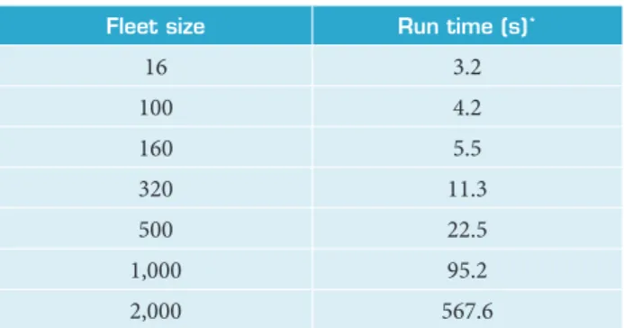
Table 1. Mo del run times for sample l eet sizes.
*Intel Core 2 Duo, 3 GHz, 16 GB RAM.
asset with more future potential than a neighboring asset will af ect the cost baseline in each subsequent year.
For generic l eets, FARM shows that the costliest aircrat possessing the lowest utility should be retired i rst. Actual l eet data show that the oldest serial numbers sometimes are not the costliest, least useful aircrat because of usage variation. h is is the most basic reason for using a methodology like the one developed for FARM in retirement analysis.
States Air Force’s Logistics, Installations and Mission Support Enterprise View repository. F-16 Fighting Falcon and A-10 h underbolt II data validated the general forms of the cost and utility models. One necessary step for validating the model was to catalog and analyze the aircrat serial numbers recommended for retirement to ensure the model accurately identii ed the weak assets. h e model was found to produce repeatable results, recommending the same serial numbers for retirement given static input conditions. Likewise, whether the l eet manager wanted to retire n aircrat or some multiple of n, the sequence of retired serial numbers remained the same.
To determine model ei cacy for an actual retirement scenario, the i scal year 2013 retirement of 41 A-10s was analyzed. More aircrat were retired during this wave, but this validation ef ort focused on the 41 aircrat sent to retirement and ignored those aircrat reassigned as maintenance and egress trainers. h e decision process to retire the 41 aircrat began in December 2011 and continued until early 2013. h e FARM model was fed with cost, utility and demographic data about the l eet in the years preceding and including 2012. Using the utility per cost ratio metric and allowing FARM to choose 41 aircrat for retirement, 19 (46%) FARM choices matched the USAF ones. Using just the cost metric resulted in 17 matches (41%) and just the utility metric resulted in 15 matches (37%). h ese validation results do not necessarily suggest that the choice of aircrat in the 2013 retirement wave was based on a utility-per-cost metric. h e stakeholders involved in the retirement used a risk-based analytical process followed by other metrics and subjective determinations to select aircrat (h omsen et al. 2011). A second A-10 retirement population was evaluated to test the model. However, the 2011 retirement wave only consisted of 9 serial numbers. Of that group, 7 were reassigned to non-l ying duties allowing only 2 serial numbers for model validation. h e model would have retired 1 of those 2 aircrat , but the small population size limits the value of the i nding. Due to the lack of additional aircrat l eet retirement data, no further validation analyses could be conducted. Retirement decisions are complex, with many subjective factors; but a simple tool that can provide decision-makers with a starting point for choosing serial numbers shows the value of this methodology. In the case of the 2013 retirement wave, FARM would have provided an initial list that was nearly 50% accurate when compared to the i nal one.
A fleet manager could employ any of the 3 retirement strategies (cost minimization, utility maximization or utility per cost maximization) used in this study. To show validity, Uncertainty
Cost data
N
o
rma
liz
e
d c
os
t
Forecast decision period [years from current]
0 0 0.2 0.4 0.6 0.8 1 1.2 1.4 1.6 1.8 2
5 10 15 20
Figure 10. Uncertainty growth for FARM decision periods.
VALIDATION
Sensitivity analysis showed accurate model response to a wide range of reasonable variable and function inputs. FARM calculated l eet retirement options for both very large and very small l eets but the results were most valuable to real-world l eet sizes in the tens to hundreds of aircrat . Computation time for all scenarios described in this article was below 60 s, and the principal component af ecting run time was the l eet size. A summary of run times for relevant USAF l eet sizes is shown in Table 1. h e model’s big O notation is: O(n2).
each strategy was compared to the others for both the A-10 case study and for a virtual leet. In each case and as expected, the named strategy outperformed the remaining ones. Figure 11 shows how the 3 strategies for the A-10 leet compare with each other for the utility-per-cost maximization strategy. he similarity between the utility-per-cost maximization and cost-minimization strategies (Fig. 11) evidences why the 2013 retirement data match well for those 2 strategies.
Other validation plots show greater stratiication between the 3 strategies. his shows the value of giving the leet manager multiple objective function options.
found that the correlation between usage history and retirement susceptibility could be better understood by leet managers. he managers can control utilization levels of their assets to prolong or accelerate deterioration, which ultimately impacts the retirement schedule. Because leet planning is a multi-year forecast, using a tool like FARM to make forecasts and periodically update them is more useful than one with a limited or inite horizon. Since suboptimal early retirement decisions cannot be remedied, a robust retirement policy is necessary.
his methodology can inspire future research in several ways. First, the methods may be extended to similar ields where parallel assets have unique usage histories. hough the objective function may change and the greedy algorithm may not present the globally optimal solution, this approach may it into other domains. Further, other domains may also wish to study the retirement problem with non-like assets. Second, this methodology did not accommodate decision-makers with complex needs. Only cost minimization, utility maximization and utility-per-cost ratio maximization were considered. An amalgamation of weighted leet priorities could be applied to this methodology, which can better satisfy some fleet managers. Lastly, future research might expand the scope of this methodology to include multiple aircrat mission designs in the retirement analysis. he F35A Joint Strike Fighter, for example, was designed to replace both the USAF’s F-16 and A-10 aircrat. Fleet managers may be interested in evaluating which mission design should be retired irst and in what quantities.
AUTHOR’S CONTRIBUTION
Newcamp J and Verhagen W conceived the idea for the study; Udlut H contributed to the methodology section and assisted with code generation; Curran R edited the text and provided the scope for the research. All authors discussed the results and commented on the manuscript.
Figure 11. Comparison of retirement strategies for utility
per cost ratio. 0
0 50 100 150 200 250 300 350
1 2 3 4 5 6 7 8
Remaining aircraft in fleet
U
ti
li
ty p
er c
os
t r
at
io
Utility per cost maximization Cost minimization
Utility maximization
CONCLUSIONS
his study applied a greedy algorithm to an aircrat leet retirement decision. It answered the question of which individual aircrat serial numbers should be retired and in what order. he hallmarks of this study were the use of inhomogeneous utilization histories for parallel assets and decision period forecasting. he methodology developed herein showed applicability to a virtual leet as well as to the current USAF A-10 leet. It was
REFERENCES
Air Force Studies Board (2011) Examination of the U.S. Air Force’s aircraft sustainment needs in the future and its strategy to meet those needs. Washington: Air Force Studies Board; The National Academies Press.
Balaban HS, Brigantic RT, Wright SA, Papatyi AF (2000) A simulation approach to estimating aircraft mission capable rates for the United States Air Force. Proceedings of the 2000 Winter Simulation Conference; Orlando, USA.
Bethuyne G (1998) Optimal replacement under variable intensity of
utilization and technological progress. Eng Economist 43(2):85-105.
doi: 10.1080/00137919808903191
Boness AJ, Schwartz AN (1969) A cost‐beneit analysis of military
aircraft replacement policies. Nav Res Logist 16(2):237-257. doi:
Carpenter M, White J (2001) Setting up a strategic architecture for the life cycle management of USAF aging aircraft. Proceedings of the RTO AVT Specialists’ Meeting on Life Management Techniques for Aging Air Vehicles; Manchester, United Kingdom.
Cormen TH, Leiserson CE, Rivest RL, Stein C (2009) Introduction to algorithms. 3rd edition. Cambridge: MIT Press.
Dixon MC; Project Air Force (U.S.) (2006) The maintenance costs of aging aircraft: insights from commercial aviation. Santa Monica: RAND Corporation Air Force.
Evans J (1989) Replacement, obsolescence and modiications of ships. Marit Pol Manag 16(3):223-231. doi: 10.1080/03088838900000061
Garcia RM (2001) Optimized procurement and retirement planning of Navy ships and aircraft; [accessed 2017 May 18]. http://calhoun. nps.edu/bitstream/handle/10945/6009/01Dec_GarciaR. pdf?sequence=1
Hartman JC (1999) A general procedure for incorporating asset utilization decisions into replacement analysis. Eng Economist 44(3):217-238. doi: 10.1080/00137919908967521
Hartman JC (2004) Multiple asset replacement analysis under variable utilization and stochastic demand. European Journal of Operational Research 159(1):145-165. doi: 10.1016/S0377-2217(03)00397-7
Hawkes EM, White III ED (2007) Predicting the cost per lying hour for the F-16 using programmatic and operational data. The Journal of Cost Analysis & Management 9(1):15-27. doi: 10.1080/15411656.2007.10462260
Hsu CI, Li HC, Liu SM, Chao CC (2011) Aircraft replacement scheduling: a dynamic programming approach. Transport Res E Logist Transport Rev 47(1):41-60. doi: 10.1016/j.tre.2010.07.006
Jardine AK, Tsang AH (2013) Maintenance, replacement, and reliability: theory and applications. Boca Raton: CRC Press.
Jin D, Kite-Powell HL (2000) Optimal leet utilization and replacement. Transport Res E Logist Transport Rev 36(1):3-20. doi: 10.1016/ S1366-5545(99)00021-6
Jones PC, Zydiak JL, Hopp WJ (1991) Parallel machine replacement. Naval Research Logistics 38(3):351-365. doi: 10.1002/1520-6750(199106)38:3<351::AID-NAV3220380306>3.0.CO;2-U
Landry N (2000) The Canadian Air Force Experience: selecting aircraft life extension as the most economical solution; [accessed 2017 May 18]. http://www.dtic.mil/docs/citations/ADP010316
Lincoln JW, Melliere RA (1999) Economic life determination for a military aircraft. J Aircraft 36(5):737-742. doi: 10.2514/2.2512
Lu L, Anderson-Cook CM (2015) Improving reliability understanding through estimation and prediction with usage information. Qual Eng 27(3):304-316. doi: 10.1080/08982112.2014.990033
Malcomson JM (1979) Optimal replacement policy and approximate replacement rules. Applied Economics 11(4):405-414. doi: 10.1080/758538855
Marx J (2016) A-10 Maintenance Oficer and Retirement Specialist. Telephone interview by Jeffrey Newcamp.
Molent L, Barter S, Foster W (2012) Veriication of an individual aircraft fatigue monitoring system. Int J Fatig 43:128-133. doi: 10.1016/j.ijfatigue.2012.03.003
Nair SK, Hopp WJ (1992) A model for equipment replacement due to technological obsolescence. Eur J Oper Res 63(2):207-221. doi: 10.1016/0377-2217(92)90026-6
Newcamp J, Verhagen W, Curran R (2016) Correlation of mission type to cyclic loading as a basis for agile military aircraft asset management. J Aero Sci Tech 55:111-119. doi: 10.1016/j.ast.2016.05.022
Peters W (1956) Notes on the Theory of Replacement. The Manchester School 24(3):270-288. doi: 10.1111/j.1467-9957.1956.tb00987.x
Rajagopalan S (1998) Capacity expansion and equipment replacement: a uniied approach. Oper Res 46(6):846-857. doi: 10.1287/ opre.46.6.846
Robbert AA, Project Air Force (U.S.), RAND Corporation (2013) Costs of lying units in Air Force active and reserve components. Santa Monica: RAND Corporation.
Stuivenberg T, Ghobbar AA, Tinga T, Curran R (2013) Towards a usage driven maintenance concept: improving maintenance value. In: Stjepandić J, Rock G, Bil C, International Society for Productivity Enhancement, editors. Concurrent engineering approaches for sustainable product development in a multi-disciplinary environment. London: Springer. p. 355-365.
Tang CH (2013) A replacement schedule model for airborne service helicopters. Comput Ind Eng 64(4):1061-1073. doi: 10.1016/j. cie.2013.02.001
Thomsen M, Whitman Z, Pilarczyk R, Clark P (2011) Development of a quantitative risk based maintenance prioritization concept. Proceedings of the Aircraft Airworthiness and Sustainment Conference; San Diego, USA.