Improving semi-automated glacial mapping with a multi-method approach: areal changes in Central Asia

(1)

TCD

8, 5433–5483, 2014

Glacier changes in Central Asia

T. Smith et al.

Title Page

Abstract Introduction

Conclusions References

Tables Figures

◭ ◮

Back Close

Full Screen / Esc

Printer-friendly Version Interactive Discussion

Discussion

P

a

per

|

Discus

sion

P

a

per

|

Discussion

P

a

per

|

Discussion

P

a

per

|

The Cryosphere Discuss., 8, 5433–5483, 2014 www.the-cryosphere-discuss.net/8/5433/2014/ doi:10.5194/tcd-8-5433-2014

This discussion paper is/has been under review for the journal The Cryosphere (TC). Please refer to the corresponding final paper in TC if available.

Improving semi-automated glacial

mapping with a multi-method approach:

areal changes in Central Asia

T. Smith1, B. Bookhagen1, and F. Cannon2

1

Institute of Earth and Environmental Science, Universität Potsdam, Potsdam, Germany

2

Geography Department, University of California, Santa Barbara, USA

Received: 31 July 2014 – Accepted: 25 September 2014 – Published: 17 October 2014

Correspondence to: T. Smith ([email protected]) and B. Bookhagen ([email protected])

(2)

TCD

8, 5433–5483, 2014

T. Smith et al.

Title Page

Tables Figures

◭ ◮

Back Close

Full Screen / Esc

Discussion

P

a

per

|

Discus

sion

P

a

per

|

Discussion

P

a

per

|

Discussion

P

a

per

|

Abstract

Central Asia has been strongly impacted by climate change, and will continue to be im-pacted by diverse climate stressors in the coming decades. This study aims to decipher the impact of climate change on glaciers in the central Tien Shan Mountain Range, a large and understudied region located northeast from the Pamir Knot.

5

To address glacier characteristics over a wide swath of Central Asia, the authors designed and implemented a glacial mapping algorithm which delineates both clean glacial ice – methods which are well documented – and glacial debris tongues, which often require extensive manual digitization. This research improves upon methods de-veloped to automatically delineate glacial areas using spectral, topographic, velocity,

10

and spatial relationships. The authors found that the algorithm misclassifies between 2 and 10 % of glacial areas, as compared to a∼750 glacier control dataset.

After validating the algorithm against multiple manually digitized control datasets, the authors applied it to a study area encompassing eight Landsat scene footprints stretching from the central Pamir through the central Tien Shan. A statistically

signifi-15

cant, though minor, gradient in glacier area loss was found, where glaciers in the west of the study area have shrunk less than those glaciers in the east. This gradient is explained by diﬀ_{erences in regional climate, where extratropical cyclones propagating}

from the west weaken and disband under continued topographic influence, as well as diﬀ_{erences in topography, where high-elevation glaciers are thermally insulated from}

20

some of the impacts of changing temperatures in the region.

1 Introduction

A combination of changing weather patterns and shrinking glaciers has begun to im-pact water resources in Central Asia. The rate, extent, and mechanisms of these changes are poorly quantified due to a lack of data and process understanding.

25

(3)

TCD

8, 5433–5483, 2014

T. Smith et al.

Title Page

Tables Figures

◭ ◮

Back Close

Full Screen / Esc

Discussion

P

a

per

|

Discus

sion

P

a

per

|

Discussion

P

a

per

|

Discussion

P

a

per

|

Pamir Ranges by providing meltwater after periods of snowmelt and before major rains. Increased understanding of changes in these glaciers is essential for sustainable water management, and mitigating the impacts of climate change on populations in Central Asia.

Changes in glacier length have long been considered one of the best indications

5

of climate change (i.e. Oerlemans, 2005), though more recent studies have also as-sessed glacial volume changes with the advent of new remote sensing techniques (e.g., Berthier et al., 2007; Aizen et al., 2007; Gardelle et al., 2012, 2013; Bolch et al., 2012; Kääb et al., 2012; IPCC, 2013). This study focuses on assessing glacial length fluctuations over a large spatial scale using publicly available remotely sensed data.

10

Several attempts have been made to produce accurate and high-resolution glacial out-lines, most notably the Global Land Ice Measurements from Space (GLIMS) project (Armstrong et al., 2005; Raup et al., 2007, 2014), and the recently produced supple-mental GLIMS dataset known as the Randolph Glacial Inventory (RGI) V3.2 (Arendt et al., 2012; Pfeﬀ_{er et al., 2014). A coherent, complete, and accurate global glacial}

15

database is important for several reasons, including monitoring global glacial changes driven by climate change, natural hazard detection and assessment, and assessment of the role of glaciers in natural and built environments, including glacial contributions to regional water budgets and hydrologic cycles (Racoviteanu et al., 2009). Precision in glacial outlines is of utmost importance for monitoring changes in glaciers, which

20

may only change by 15–30 m yr−1 (∼1–2 pixels of Landsat Enhanced Thematic Map-per (ETM+_{) yr}−1_{). Thus, spatially accurate glacial outlines are imperative for precise}

glacial change detection (Paul et al., 2004, 2013).

Several methods have been developed to delineate clean glacial ice (i.e. Paul, 2002; Paul et al., 2002; Racoviteanu et al., 2008a, b; Hanshaw and Bookhagen, 2014),

25

(4)

TCD

8, 5433–5483, 2014

T. Smith et al.

Title Page

Tables Figures

◭ ◮

Back Close

Full Screen / Esc

Discussion

P

a

per

|

Discus

sion

P

a

per

|

Discussion

P

a

per

|

Discussion

P

a

per

|

grain size (i.e. Dozier, 1989; Painter et al., 2003, 2009; Dozier and Painter, 2004). Analysis of seasonal snow cover throughout the study area is based on these studies; snow cover is an important climatic indicator used in assessing trends in snow-covered area across Central Asia.

Although significant progress has been made towards automated glacial outline

5

retrieval using satellite imagery, these methods struggle to accurately map debris-covered glaciers or other glaciers with irregular spectral profiles (Paul et al., 2004; Bolch et al., 2007; Racoviteanu et al., 2008b; Scherler et al., 2011a). Much of this diﬃ

-culty stems from the similarities in spectral profiles of debris located on top of a glacial tongue and the surrounding hillslopes from which the debris is sourced. The majority

10

of studies examining debris-covered glaciers employ extensive manual digitization in a Geographic Information System (GIS), which is very time consuming, and can in-troduce significant user-generated errors (Paul et al., 2013; Pfeﬀ_{er et al., 2014; Raup}

et al., 2014). Building on the multi-spectral, topographic, and spatially-weighted meth-ods developed by Paul et al. (2004), the authors present a refined rules-based

classi-15

fication based on spectral, topographic, land-cover, velocity, and spatial relationships between glacial areas and the surrounding environment.

Using a suite of 62 Landsat Thematic Mapper (TM), Enhanced Thematic Mapper+

(ETM+_{) and Optical Land Imager (OLI) images across a spatially and topographically}

diverse set of study sites comprising eight Landsat footprints (path/row combinations:

20

144/30, 145/30, 147/31, 148/31, 149/31, 151/33, 152/32, 153/33) along a profile from the central Pamir to the central and central-eastern Tien Shan (Fig. 1), the authors (1) pre-process the imagery (georeference and co-register), (2) apply the algorithm based on spectral, topographic, velocity, and spatial information, (3) analyze range-wide trends in glacial character, and (4) link spatially heterogeneous glacial area loss to

25

(5)

TCD

8, 5433–5483, 2014

T. Smith et al.

Title Page

Tables Figures

◭ ◮

Back Close

Full Screen / Esc

Discussion

P

a

per

|

Discus

sion

P

a

per

|

Discussion

P

a

per

|

Discussion

P

a

per

|

2 Study area and data sources

2.1 Study area

The wintertime climate of the study area is controlled by both the Winter Westerly Dis-turbances (WWDs) and the Siberian High, which dominate regional circulation and cre-ate strong precipitation gradients throughout the Tien Shan Range, which extends from

5

Uzbekistan in the west through China in the east (Fig. 1) (Lioubimtseva and Henebry, 2009; Narama et al., 2010; Bolch et al., 2011; Sorg et al., 2012; Cannon et al., 2014). The western edges of the study region tend to receive more winter precipitation in the form of snow, with precipitation concentrated in the spring and summer in the central and eastern reaches of the range (Narama et al., 2010).

10

Sorg et al. (2012) note that due to the interaction of the Siberian High – a semi-permanent thermal high-pressure system that extends from Siberia towards the Tien Shan – and more western continental atmospheric patterns such as WWDs, the study area has a distinct precipitation gradient with decreasing precipitation from the west to east. There is also a strong gradient between outer and inner reaches of the Tien

15

Shan, as moisture is precipitated on the windward (outer) side of topography, moving eastwards from the Pamirs (Sorg et al., 2012).

Several smaller-scale studies have examined glacial changes in the Tien Shan (e.g., Aizen et al., 1997, 2006; Narama et al., 2006, 2010; Shangguan et al., 2009; Osmonov et al., 2013). Narama et al. (2010) found that for the period of 1970–2010, glacial

20

area decreased between 9 and 19 %, depending on the subregion of the Tien Shan analyzed. Glacial loss was then seen to accelerate between 2000 and 2007, except in a few cases in the southeastern reaches of the Tien Shan (Narama et al., 2010). This agrees generally with work by Narama et al. (2006), who noted that total glaciated area in the northern and central Tien Shan had shrunk by 14.2 % between the 1860s and

25

(6)

TCD

8, 5433–5483, 2014

T. Smith et al.

Title Page

Tables Figures

◭ ◮

Back Close

Full Screen / Esc

Discussion

P

a

per

|

Discus

sion

P

a

per

|

Discussion

P

a

per

|

Discussion

P

a

per

|

and mechanisms of glacial change in the region, as well as potential linkages between diﬀ_{erences in area loss rates and local or regional climate.}

2.2 Data sources

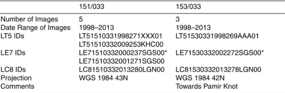
Our glacial mapping algorithm is based on several datasets. The Landsat 5 (TM), 7 (ETM+_{), and 8 (OLI) platforms were chosen as the primary spectral data sources, as}

5

they provide spatially and temporally extensive coverage of the study area (Table 1). ASTER can also be used as a source of spectral information, but here the authors chose to focus on the larger footprint and longer timeseries available through the Land-sat archive. In addition to spectral data, the 2000 Shuttle Radar Topography Mission (SRTM) Digital Elevation Model (DEM) (∼90 m) was leveraged to provide elevation,

10

slope, and hillshade information (Farr and Kobrick, 2000). The SRTM data and its derivatives were downsampled to 30 m to match the resolution of the Landsat images using bilinear resampling. The USGS Hydrosheds river network (15 s resolution) was also used as an input dataset (Lehner et al., 2008).

Several climatic datasets were analyzed to provide context to the analysis of glacial

15

changes in the study area. Daily gridded Advanced Microwave Scanning Radiometer (AMSR-E) data (0.25◦×0.25◦resolution) was used to estimate the snow–water

equiv-alent (SWE) stored throughout the study area on a yearly basis (2002–2011) (Tedesco et al., 2004). The AMSR-E satellite measures microwave brightness temperatures at diﬀ_{erent frequencies to analyze snow depth, although the algorithm assumes a}

ho-20

mogeneous snowpack with constant grain size (Tedesco and Narvekar, 2010). SWE measurements are further complicated by changing snow densities, which are not well represented in the AMSR-E dataset, because it converts estimated snow depth to a wa-ter equivalent. Despite these caveats, the AMSR-E SWE measurements remain the best estimates of the water stored in snowpack throughout much of the world, and

25

especially in remote and understudied areas such as the Tien Shan.

(7)

TCD

8, 5433–5483, 2014

T. Smith et al.

Title Page

Tables Figures

◭ ◮

Back Close

Full Screen / Esc

Discussion

P

a

per

|

Discus

sion

P

a

per

|

Discussion

P

a

per

|

Discussion

P

a

per

|

(1998–2014), were used to analyze precipitation across the range (Huﬀ_{man et al.,}

2010; Bookhagen, 2010; Bookhagen and Burbank, 2010; Duan and Bastiaanssen, 2013). The precipitation radar (PR) onboard TRMM primarily senses rainfall, as liquid water is easier to detect by radar, although the TRMM datasets used in this study also contain information from several other datasets (e.g., AMSR-E precipitation estimates,

5

infrared (IR) imagery from several satellites including Geosynchronous Operational En-vironmental Satellites (GOES), Multifunctional Transport Satellite (MTSat), and Meteo-rological Satellite (Meteosat), Advanced Microwave Sounding Unit (AMSU-B), as well as Global Precipitation Climatology Centre (GPCC) ground-based rainfall measure-ments), which are merged during processing to improve precipitation estimates (Huﬀ

-10

man and Bolvin, 2007).

Two Moderate Resolution Imaging Spectroradiometer (MODIS) products, MOD10C1 (snow covered area, SCA) and MOD11C1 (land surface temperature, LST) were used to analyze yearly average snowcover and atmospheric lapse rates respectively (Hall and Salomonson, 2006; Wan, 2008). MOD10C1 data between 2001 and 2014 were

15

aggregated to seasonal timesteps at 0.05◦×0.05◦ spatial resolution. MOD11C1 data

was aggregated seasonally to calculate atmospheric lapse rates at 0.05◦×0.05◦spatial

resolution using SRTM elevation data. Lapse rates were calculated using night time temperatures, which have been shown to be more consistent in alpine regions (Colombi et al., 2007). A recent study validated MODIS LST data in the region by comparing

20

ground station data for western Tibet with generated LST products, finding generally good agreement across both day and night (Wang et al., 2007).

Daily Climate Forecast System Reanalysis (CFSR) data were obtained at 0.5◦×0.5◦

spatial resolution over the time period 1979–2010 (Saha et al., 2010). The dataset was chosen on account of its model coupling, spatial resolution, and modern assimilation

25

(8)

TCD

8, 5433–5483, 2014

T. Smith et al.

Title Page

Tables Figures

◭ ◮

Back Close

Full Screen / Esc

Discussion

P

a

per

|

Discus

sion

P

a

per

|

Discussion

P

a

per

|

Discussion

P

a

per

|

was developed for the study region to inform analysis of changes in glacier character throughout the range.

It is important to note the lack of climate station data in the study region, especially at high elevations (Schöne et al., 2013). Previous studies in the region (e.g, Osmonov et al., 2013) have used low elevation stations (∼3600 m), which are well below the

5

median elevation of most glaciers in the study region. Due to the extent of our study region, the authors have chosen to rely on large-scale satellite data for climate and atmospheric analysis in the place of ground station data.

The RGI V3.2 dataset is comprised of ∼198 000 glaciers with an estimated extent of 726 800±34 000 km2 (Pfeﬀer et al., 2014). This dataset was derived from previous

10

glacier inventories, as well as satellite imagery over the period of 1999–2010, and provides complete global coverage, excepting ice sheets. This dataset was intended for wide-scale analysis, and has been successfully used to improve estimates of global glacial changes, and their contribution to sea-level rise. In our study, the dataset is used as a comparison dataset against which to analyze algorithm-derived glacial outlines.

15

It is important to note, however, that the RGI was not designed for detailed glacial comparisons, and it is included in this study not because of its accuracy with specific glaciers, but rather because of its wide use in glacial analysis and its position as the most complete glacier inventory of the study area.

3 Methods

20

3.1 Data preparation

For accurate glacial delineation, the authors used primarily those Landsat images that were free of new snow, and had less than 10 % cloud cover. The presence of fresh snow in images tends to overclassify glacial areas and classify non-permanent snow as glaciers. Additionally, cloud cover tends to confuse the algorithm, and render

(9)

TCD

8, 5433–5483, 2014

T. Smith et al.

Title Page

Tables Figures

◭ ◮

Back Close

Full Screen / Esc

Discussion

P

a

per

|

Discus

sion

P

a

per

|

Discussion

P

a

per

|

Discussion

P

a

per

|

glacial outlines that overlap with cloud cover unreliable (Paul et al., 2004; Hanshaw and Bookhagen, 2014).

After selecting a series of Landsat images, the authors co-registered each image to a “master” image specific to each Landsat path/row combination, using the Auto-mated Registration and Orthorectification Package (AROP) (Gao et al., 2009). Master

5

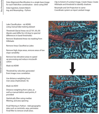
images are denoted in Table 1 with an asterisk. This ensures that glacier outlines are properly matched, and that any timeseries of glacial change is consistent in space. Once the data were georeferenced and registered, a series of scripts written in Python and Matlab performed the glacier classification (flow diagram shown in Fig. 2, source code available at: http://www.github.com/ttsmith89/GlacierExtraction/). The algorithm

10

uses Landsat imagery, a hydrologically corrected DEM, a velocity surface derived from image cross-correlation, and the Hydrosheds 15 s river network (buﬀ_{ered by 200 m}

and converted to a raster) as the primary inputs. A script prepares these datasets for processing by resampling and reprojecting each dataset to the same spatial extent, resolution (30 m to match the Landsat data), and projection. It further generates slope

15

and hillshade images from the DEM, and rectifies additional input datasets described below. Although the current algorithm is based on proprietary software, the authors will continue to update the code with the goal of using only open source tools and libraries in the future.

3.2 Lake delineation

20

Glacial debris tongues tend to host supra-glacial lakes, particularly during the summer months when snow cover is lowest (Quincey et al., 2007; Gardelle et al., 2011). These lakes can be used as seed points for distance-weighting mechanisms to more accu-rately delineate glacial debris tongues. Lakes are delineated using the Normalized Dif-ference Water Index (NDWI) (Gao, 1996), after which misclassified areas are removed

25

(10)

TCD

8, 5433–5483, 2014

T. Smith et al.

Title Page

Tables Figures

◭ ◮

Back Close

Full Screen / Esc

Discussion

P

a

per

|

Discus

sion

P

a

per

|

Discussion

P

a

per

|

Discussion

P

a

per

|

instead used a manually generated set of index lakes that exhibit the spectral proper-ties desired. This small manual step greatly increases the number of correctly classified lakes by providing scene-specific NDWI thresholds for each processed image.

3.3 Glacier delineation

3.3.1 Spectral delineation

5

Calculations are performed on rasterized versions of each input dataset, which have been standardized to the same matrix size. The first step in the classification process leverages Landsat Bands 1, 3, and 5. For Landsat 8 OLI images, a slightly diﬀ_erent

set of bands is used to conform to the modified spectral range of sensors on Landsat 8. For simplicity, bands referenced in this publication refer to Landsat 7 ETM+

spec-10

tral ranges. The ratio of TM3/TM5 (value≥2), with additional spectral information from

TM1 (value >_{250) has long been established as an e}ﬀ_{ective means of delineating}

glacier areas (e.g., Hall et al., 1987; Hanshaw and Bookhagen, 2014), but is not ef-fective in delineating debris-covered glacier areas (Fig. 3). Shadowed areas derived from a SRTM-generated hillshade specific to the date and time of each Landsat image,

15

as well as lake areas derived in the previous lake processing step, are then removed from this initial spectral classification (Huggel et al., 2002; Hanshaw and Bookhagen, 2014). The end result of this step is the spectrally-derived glacier outlines, which are later integrated back into the workflow before statistical filtering.

3.3.2 Topographic filtering

20

Building on the work of Paul et al. (2004), low slope areas (between 1 and 24◦) are iso-lated as areas where debris-covered glaciers are likely to exist. As glacial surfaces tend to be rougher than the surrounding areas, a standard deviation filter (3×3 kernel size)

is also applied to the slope and used to mask out areas of low slope variability. Low elevation areas (defined on a scene-by-scene basis) are then masked out to decrease

(11)

TCD

8, 5433–5483, 2014

T. Smith et al.

Title Page

Tables Figures

◭ ◮

Back Close

Full Screen / Esc

Discussion

P

a

per

|

Discus

sion

P

a

per

|

Discussion

P

a

per

|

Discussion

P

a

per

|

processing time. These thresholding steps are performed independently of the previ-ous, spectrally delineated, glacier outlines. In essence, this step identifies areas where there is the potential for a debris-covered glacier to exist. Additional thresholding is then performed on this “potential debris area” subset to identify debris-covered glacier areas.

5

The Correlation Image Analysis Software (CIAS) tool (Kääb, 2002), which uses a method of statistical image cross-correlation, is used to derive glacial velocities from Landsat Band 8 panchromatic images. This method functions by tracking individual pixels across space and time, and provides a velocity surface at the same resolution as the input datasets (15 m). The velocity surface is then upsampled using bilinear

re-10

sampling to provide a consistent velocity estimate across the entire Landsat scene. The authors then standardized the velocity measurements to m yr−1using the capture dates of the two Landsat images. It is important to note that cloud-free and snow-free images are essential for this step, as the presence of snow or cloud cover can disrupt the correlation process, resulting in anomalous velocity measurements.

15

The authors only used one multi-year velocity measurement for each path/row com-bination to derive general areas of movement/stability for glacial classification, as using stepped velocity measurements over smaller time increments did not show a notice-able improvement in glacial classification. These velocities ranged generally from 4– 30 m yr−1across the diﬀ_{erent scenes, and were chosen based on both manual}

inspec-20

tion of the velocity surfaces, and their impact on glacial classification on a test dataset. Furthermore, a method of frequential cross-correlation using the co-registration of op-tically sensed images and correlation (COSI-Corr) tool (Leprince et al., 2007; Scherler et al., 2011b) was tested and did not show any appreciable improvement in velocity measurements (Heid and Kääb, 2012).

25

(12)

TCD

8, 5433–5483, 2014

T. Smith et al.

Title Page

Tables Figures

◭ ◮

Back Close

Full Screen / Esc

Discussion

P

a

per

|

Discus

sion

P

a

per

|

Discussion

P

a

per

|

Discussion

P

a

per

|

limited success. Some glaciers exhibited a unique frequency signature when analyzed using spatial FFTs, although these were not consistent across multiple debris-covered glaciers with diﬀ_{ering surface characteristics. Additionally, the FFT approach was tested}

against a principal component analysis (PCA) image derived from all Landsat bands, without significant improvement to the algorithm.

5

The authors also attempted to integrate surface roughness measurements using the ASTER satellite, which contains both forward looking (3N – nadir) and backwards look-ing (3B – backwards) images, primarily intended for the generation of stereoscopic DEMs. The diﬀ_{erence in imaging angle provides the opportunity to examine surface}

roughness by examining changes in shadowed areas (Mushkin et al., 2006; Mushkin

10

and Gillespie, 2011). The authors found that there are slight surface roughness diﬀ

er-ences between glaciated and non-glaciated areas on some debris tongues, but that these diﬀ_{erences are not significant enough to use as a thresholding metric.}

Further-more, the nature of the steep topography limits the eﬃ_{cacy of this method, as valleys}

that lie parallel the satellite flight path and those that lie perpendicular to the flight path

15

show diﬀ_{erent results. Thus, the algorithm relies on the velocity and slope thresholds}

to characterize the topography of the glacial areas.

The velocity step is most important for removing hard-to-classify pixels along the edges of glaciers, and wet sands in riverbeds. These regions are often spectrally indis-tinguishable from debris tongues, but have very diﬀ_{erent velocity profiles. It is}

impor-20

tant to note, however, that this step also removes some glacial area, as not all parts of a glacier are moving at the same speed. This can result in small holes in the delineated glaciers, which the algorithm attempts to rectify using statistical filtering.

3.3.3 Spatial weighting

After topographic and velocity filtering, a set of spatially weighted filters was

con-25

(13)

TCD

8, 5433–5483, 2014

T. Smith et al.

Title Page

Tables Figures

◭ ◮

Back Close

Full Screen / Esc

Discussion

P

a

per

|

Discus

sion

P

a

per

|

Discussion

P

a

per

|

Discussion

P

a

per

|

flowlines all the way to the peaks of mountains, the river network provides an ideal set of seed points with which to remove misclassified pixels. A second distance weighting is then performed using both the supra-glacial lakes detected during the lake delineation step, and the spectrally delineated glaciers. As debris tongues must occur in proximity to one or more of: (1) glacier areas, (2) the centerlines of valleys, or (3) supra-glacial

5

lakes, this step is eﬀ_{ective at removing overclassified areas. At this step, it is also}

possible to add manual seed points, which may be necessary for some longer debris tongues. The authors note that these are optional, and the majority of glaciers do not need the addition of manual seed points. However, for certain glaciers that do not have many lakes, or do not have lakes large enough to be delineated by Landsat, adding

10

a few manual control points greatly increases the eﬃ_{cacy of the algorithm.}

The spatial weighting step is essential for removing pixels that are spatially distant from any glacier or lake area. In many cases, large numbers of river pixels, and in some cases dry sand pixels, have similar spectral and topographic profiles to debris covered glaciers. This step eﬀ_{ectively removes the majority of pixels outside the general}

15

glaciated area(s) of a Landsat scene.

3.3.4 Masking and filtering

Once the spatial weighting steps are completed, the glacial outlines are generally accu-rate. Additional filtering and smoothing steps help to remove some misclassified pixels due to errors in the SRTM DEM, high velocities in non-glacier areas, and areas with

20

similar spectral profiles to glaciers. An NDWI mask is applied to remove dry areas, as glaciers uniformly exhibit a moisture signal that is detectable with NDWI. A Normal-ized Diﬀ_{erence Vegetation Index (NDVI) mask is also applied, as glaciers in the study}

region rarely have noticeable vegetation. The authors note that all of the threshold pa-rameters are set on the basis of Landsat scene path/row combinations to account for

25

the slightly diﬀ_{erent topographic, velocity, and landcover settings of spatially diverse}

Landsat scenes. In general, one set of parameters is suﬃ_{cient to characterize glaciers}

(14)

TCD

8, 5433–5483, 2014

T. Smith et al.

Title Page

Tables Figures

◭ ◮

Back Close

Full Screen / Esc

Discussion

P

a

per

|

Discus

sion

P

a

per

|

Discussion

P

a

per

|

Discussion

P

a

per

|

throughout time. However, scenes with extensive cloud cover or snow cover some-times need separate thresholds to account for the diﬀ_{erences in spectral signatures}

between cloud-free and cloud-covered images.

A set of median filters are then applied, as well as a set of statistical filters designed to remove isolated pixels (3×3 median filter, applied twice, as well as 5×5 median

5

filter, applied after image opening), bridge gaps between isolated glacial areas (image bridging), and fill holes in large contiguous areas (image opening, applied twice). After these filters have been applied, the resulting glacial outlines are post-processed in order to add metadata to each glacier, remove very small glacial areas (∼10–20 px or

less), and export the results in vector format.

10

This step is essential for filling holes and reconnecting separated glacier areas. As the filtering methods used are based on a fixed set of threshold values, there are often glacier pixels that are removed. For example, some pixels along the edge of a de-bris tongue may be moving slower than the provided velocity threshold, and are thus removed. This problem is somewhat, but not completely, remedied by the statistical

15

filtering (Fig. 4).

3.4 Creation of manual control datasets

Two manual control datasets encompassing ∼750 glaciers (∼3000 km2) each were

created to test the eﬃ_{cacy of the glacial mapping algorithm. The authors note that}

although the manual datasets here are considered “perfect”, there is inherent error in

20

any manual digitization in a GIS (e.g., Paul et al., 2013). Due to the lack of ground truth information, the authors have estimated the overall uncertainty of the manual dataset to be 2 % (Paul et al., 2002, 2013).

Before any comparisons between glaciers can be performed, contiguous glacial ar-eas – both due to snowcover and to ice caps – must be split into component parts.

25

(15)

TCD

8, 5433–5483, 2014

T. Smith et al.

Title Page

Tables Figures

◭ ◮

Back Close

Full Screen / Esc

Discussion

P

a

per

|

Discus

sion

P

a

per

|

Discussion

P

a

per

|

Discussion

P

a

per

|

the diverse datasets and classified glacial areas can be split into the same subset areas for statistical comparison.

4 Results

4.1 Statistical analysis of algorithm errors

A subset of 138 glaciers from the two manual control datasets of varying size and

5

topographic setting was chosen for more detailed analysis. The unedited, algorithm-generated, glacial outlines were compared against three separate datasets: (1) the RGI V3.2 (Arendt et al., 2012), which is considered due to its position as the most complete and accurate global glacial database; (2) spectral outlines, which only classify the glacial areas via commonly used spectral subsetting (using TM1, TM3, and TM5);

10

and (3) a manual control dataset, which was hand-digitized by the authors from Landsat imagery. Figure 5 shows the bulk elevation distributions across 138 glaciers for each dataset in 10 m elevation bins. An additional set of figures showing the eﬀ_{ects of each}

step of the algorithm on glacier classification are available in the Supplement.

From these distributions, it is apparent that the RGI universally overclassifies glacial

15

areas, and that using only a spectral classification tends to overclassify high-elevation areas and underclassify low-elevation areas. It is important to note that the RGI was not intended for direct glacial comparisons as it is used here. The authors use it here as the best publicly available glacial database against which to compare our results over a large area. There is some apparent bias in the authors’ algorithm towards

low-20

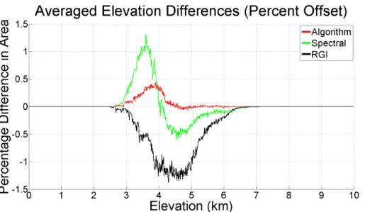
elevation areas, which represent the debris-covered portions of glaciers and are the most diﬃ_{cult areas to classify. To illustrate the di}ﬀ_{erence between the manual control}

dataset and each of the comparison datasets, the elevation distributions were diﬀ

er-enced in Fig. 6.

In general, the same patterns appear in Fig. 6 as in Fig. 5: that is, the spectral-only

25

(16)

TCD

8, 5433–5483, 2014

T. Smith et al.

Title Page

Tables Figures

◭ ◮

Back Close

Full Screen / Esc

Discussion

P

a

per

|

Discus

sion

P

a

per

|

Discussion

P

a

per

|

Discussion

P

a

per

|

algorithm-derived dataset underclassifies low-elevation areas. However, at any given elevation slice, the algorithm-derived data were oﬀ _{by less than 0.5 % from the area}

of the manual control dataset, and are generally well matched at elevations above 4000 m. The underclassification at the 3500–4000 m class can be attributed to hard-to-classify side glaciers, or tributary glaciers. Many of these glaciers are located in shaded

5

or otherwise topographically distinct valleys, which can result in underclassification of connected glacial areas, although an analysis of shadowed-area mismatches between manual and algorithm datasets indicates that shadowed areas are responsible for only very small misclassifications (∼4×10−8km2,∼5–10 px per elevation slice). Over the span of a single Landsat scene, or even over most individual watersheds within a

Land-10

sat scene, the elevation distributions of the manual and algorithm datasets are virtually indistinguishable (ks-test at the 99 % confidence interval passes).

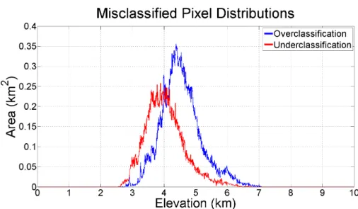
In order to examine persistent bias throughout the algorithm classification, under-and over-classified areas were examined. To determine areas of overclassification (un-derclassification), the manually (algorithm) generated dataset was subtracted from the

15

algorithm (manual) dataset, leaving only pixels that were overclassified (underclassi-fied). Figure 7 shows the elevation distributions of under- and over-classified areas. The algorithm tends to consistently overclassify areas above 4500 m, and underclas-sify areas under 4500 m, though much of this misclassification occurs at similar eleva-tion slices, and thus in bulk the mismatch between the manual and algorithm derived

20

datasets is minimal. The total misclassification of algorithm-derived outlines against the two control datasets is 2 and 10 % respectively, which represents a significant improve-ment from a pure spectral delineation approach. The authors would like to emphasize that these oﬀ_{sets refer to the unedited algorithm-derived outlines, before any manual}

corrections have been applied.

25

(17)

TCD

8, 5433–5483, 2014

T. Smith et al.

Title Page

Tables Figures

◭ ◮

Back Close

Full Screen / Esc

Discussion

P

a

per

|

Discus

sion

P

a

per

|

Discussion

P

a

per

|

Discussion

P

a

per

|

lower-elevation areas vs higher-elevation areas, and underclassifying lower-slope ar-eas. These are known errors associated with the diﬃ_{culty of classifying glacial tongues,}

particularly those with heavy debris cover. However, on average, the mismatch between the algorithm and manual control datasets is minimal regardless of topographic setting (between 2–10 %). It is important to note that the algorithm datasets used in the

sta-5

tistical analysis were not manually edited, and are the direct output of the authors’ algorithm.

4.2 Comparison to a random sampling of glacial areas

In order to examine sampling bias in our analysis, the researchers used 465 GLIMS glacier identification numbers (centroids, point features) that overlapped with the

man-10

ual control datasets. A random subset of 100 of these points was chosen for this anal-ysis. As can be seen in Fig. 9, similar patterns emerge between the randomly sampled glaciers and the sampling used in other sections of this manuscript. There is evidence of increased noise in the random sample, as some glaciers that were avoided by the researchers due to closeness to wet sand or other hard-to-classify areas were chosen

15

during the random sampling. However, in general, the relationship between the algo-rithm and the manual datasets remains significant (ks-test passes at 99 % confidence interval).

5 Discussion

Using the newly developed glacier delineation algorithm, the authors analyzed

shrink-20

age rates of glaciers from the central Pamir through the most heavily glaciated region of the Tien Shan (Fig. 1). Minimal manual inspection and rectification was performed on glaciers used in the areal-change analyses, to ensure that algorithm errors were not propagated into the discussion of glacier change. A dataset of 313 glaciers was used to examine shrinkage trends across the study area.

(18)

TCD

8, 5433–5483, 2014

T. Smith et al.

Title Page

Tables Figures

◭ ◮

Back Close

Full Screen / Esc

Discussion

P

a

per

|

Discus

sion

P

a

per

|

Discussion

P

a

per

|

Discussion

P

a

per

|

5.1 Area loss in selected glaciers

Two example glaciers were chosen to display specific area changes (Figs. 10 and 11). Both, glaciers have lost area over the period 1998–2014. Including additional data sources such as Corona, Landsat Multispectral Scanner (MSS), ASTER, and non-cloud-free Landsat TM, ETM+_{and OLI images was outside of the scope of this study.}

5

The authors would like to note that the primary use of the algorithm is in assess-ing trends at a larger spatial scale, usassess-ing dozens of glaciers, and not in assessassess-ing trends within individual glaciers. Due to the diﬃ_{culties inherent in dividing one glacier}

area from another, particularly at high-elevation areas where snowcover often connects multiple glaciers, area changes on a glacier-by-glacier basis are associated with larger

10

uncertainties and require significant manual work to separate combined glacial area into individual glaciers. Furthermore, over- and under-classified areas, which tend to even out over a large spatial scale, can present problems at the scale of individual glaciers, especially in complex terrain or in the case of debris-covered glaciers. An eﬀ_{ort was made to choose glaciers that are somewhat isolated to demonstrate areal}

15

changes at a small scale, using both the algorithm and some manual corrections at the glacial tongue. The algorithm is most useful when glacier area changes are assessed at a watershed, drainage basin, or range-wide scale.

5.2 Areal changes in glaciers in the study area

The total mapped glacier area across the eight Landsat scene footprints used in this

20

study was approximately 9444.7±189 km2circa the year 2000, with 4376.75 km2 man-ually inspected, edited, and used for statistical analysis. The bulk area loss rate across glaciers that were quality controlled was 3.9 % (total area loss of 172.24 km2over the period∼1999 to∼2014). The area loss rates across the study area vary widely and

can change significantly within the confines of a single Landsat scene footprint.

Fur-25

(19)

TCD

8, 5433–5483, 2014

T. Smith et al.

Title Page

Tables Figures

◭ ◮

Back Close

Full Screen / Esc

Discussion

P

a

per

|

Discus

sion

P

a

per

|

Discussion

P

a

per

|

Discussion

P

a

per

|

for the whole study area diﬃ_{cult, and thus our 3.9 % shrinkage rate represents only an}

estimate of the total area loss in glaciers in the study area.

5.2.1 Relationship with previous studies

Several smaller scale studies have examined glaciers and glaciated areas that overlap with our study area. Using both raw and minimally corrected algorithm-derived glacier

5

outlines, the authors have compared our area change rates for selected areas with those previously published in the literature. These values are presented in Table 2. The authors note that the shrinkage rates established in previous studies (with the exception of Osmonov et al., 2013) do not generally overlap our data in time and are thus diﬃ_cult

to compare. However, the area loss rates established in this study are comparable to

10

those published in the literature, albeit with a slight increase in melt rates over the last decade, as noted previously by Aizen et al. (2006) and Narama et al. (2010).

5.2.2 Area loss rate gradient across the study area

Figure 12 illustrates the relationship between geographic location, from west to east, and areal changes across the study area. Although noise in the data is evident, all

15

of the data were generated using the same methodology, and are thus comparable. The gradient of the fitted line is 7×10−4km2yr−1m−1per decimal degree; at_test

per-formed on the data shows that the trend is significant at the 95 % confidence level. The one caveat to this is that the authors have noted that not all Landsat scenes per-form equally; scenes with excess snow, cloud cover, shadows, or other strong spectral

20

signatures may lead to the misclassification of some glacial areas. The authors have also noted that OLI images generally perform better than TM or ETM+_images,

par-ticularly in images with cloud and snow cover. However, this relationship has not been substantiated with thorough statistical analysis, and should not be considered definite. The authors posit that the increased pixel depth with the 12-bit dynamic range

sen-25

(20)

TCD

8, 5433–5483, 2014

T. Smith et al.

Title Page

Tables Figures

◭ ◮

Back Close

Full Screen / Esc

Discussion

P

a

per

|

Discus

sion

P

a

per

|

Discussion

P

a

per

|

Discussion

P

a

per

|

decreased image saturation, but this relationship remains speculative. An eﬀ_{ort was}

made to choose only the best suited images for this study; as can be seen from the statistical analysis presented above, the glacier outlines are generally accurate, par-ticularly when considered in larger quantities. Any scenes with cloudcover used in this analysis have been visually inspected and manually corrected.

5

Regional bulk areal change rates do not necessarily represent an accurate account-ing of glacial health – for example, high-elevation glaciers will generally change more slowly than low-elevation glaciers. This research has chosen to normalize the areal change rate data by the median elevation of each glacier (Hanshaw and Bookhagen, 2014). When the data are normalized by other indices, such as median slope and area,

10

the relationship remains consistent, in that glaciers further to the east in the study area tend to have shrunk more than glaciers to the west, over the period ∼1998–2014. When low-elevation glaciers (median elevation<_{4000 m) are analyzed independently,}

areal change rates across the study area do not show a gradient, in that there is not significant variation from west to east. Glaciers above 4000 m, and in each individual

15

elevation slice above that (broken into 250 m slices) show the same east/west gradient in areal change as the complete glacier dataset albeit, with varying longitudinal trends. The gradient in glacial area changes agrees well with work by Gardelle et al. (2013), who noted that the Pamir Range has experienced slightly positive mass balances over the period 2000–2011. Although this study is focused on areal changes as opposed to

20

the mass balances examined by Gardelle et al. (2013), the authors propose a similar mechanism for the variability in glacial area change rates: spatial gradients in precip-itation. To understand climatic forcing across the range, the authors have analyzed several climatic and topographic variables to determine the factors responsible for the variation in change rates across the study area.

(21)

TCD

8, 5433–5483, 2014

T. Smith et al.

Title Page

Tables Figures

◭ ◮

Back Close

Full Screen / Esc

Discussion

P

a

per

|

Discus

sion

P

a

per

|

Discussion

P

a

per

|

Discussion

P

a

per

|

5.3 Climatic influences

To analyze the impacts of climatic gradients across the study area on glacial behavior, the authors created a swath profile from the central Pamir through the central Tien Shan.

Figure 13a and b shows the general topography across the range from the Pamir

5

Knot towards the eastern end of the Tien Shan. The highest elevation areas host the most glaciers, most notably the Pamirs on the west of the swath profile (∼73◦E) and

the area surrounding the Inylchek glacier∼80◦E. Both SWE and precipitation in gen-eral are fairly low (<_{200 mm yr}−1_{) throughout the range. Figure 13c shows precipitation}

and snow cover throughout the study area, as well as seasonal precipitation

percent-10

ages. Winter (November–April) precipitation is dominant up until the eastern edge of the Pamirs, where summer (May–October) precipitation becomes dominant. As glacial response to summer and winter precipitation regimes is diﬀ_{erent (e.g., Narama et al.,}

2010), the split between the winter and summer growth regions could also explain some of the east-west variability in glacier area loss. This theory is also supported by

15

the lack of east-west area loss gradient in low-elevation glaciers (<_{4000 m), which are}

most strongly influenced by increasing temperatures in the region. Glaciers above this zone, which have also experienced shrinkage, receive relatively more snowfall, and are thus more sensitive to regional weather patterns’ influence on precipitation.

The atmospheric lapse rates (Fig. 13d) illustrate generally cold temperatures year

20

round in the Pamirs, and generally higher summer temperatures than winter tempera-tures throughout the remainder of the study area. Lapse rates are defined here as the change in atmospheric temperature (in this case, night-time land surface temperature, MODIS product MOD11C) over change in elevation, which gives a temperature gradi-ent across the mountain range. The strongly negative lapse rates in the west indicate

25

(22)

TCD

8, 5433–5483, 2014

T. Smith et al.

Title Page

Tables Figures

◭ ◮

Back Close

Full Screen / Esc

Discussion

P

a

per

|

Discus

sion

P

a

per

|

Discussion

P

a

per

|

Discussion

P

a

per

|

impacted by warming temperatures, as they are situated in generally warmer areas to begin with.

There is a distinct precipitation gradient between the external watersheds and the internal watershed, which drains towards the Taklamakan Desert (generalized into in-ternal and exin-ternal components as a black line in Fig. 13a). The inner basin receives

5

less rainfall, and has less snow covered area. Lapse rates are similar in the two re-gions, primarily due to generally cold temperatures year round. Unfortunately, TRMM 3B43 (or 3B42) data did not allow the authors to eﬀ_{ectively measure snowfall (Palazzi}

et al., 2013), which is a key component in glacier area changes, and there is insuﬃ_cient

data to draw conclusions on whether or not the drainage divide influences glacier area

10

change rates. It is unlikely that the north-south divide is as strong of a control on glacial areas in the region as the east-west gradient.

5.4 Atmospheric setting

We have identified an east to west gradient in glacier area change rates, but it is not clear what factors have driven the variable changes over the past∼16 yrs. To assess

15

the influence of climate in this region, the authors have focused on atmospheric cir-culation and precipitation to create lag-composites detailing the impacts of wintertime extra-tropical cyclones along the Pamir and Tien Shan Ranges.

The WWDs are most active between January and March (Lang and Barros, 2004), and are responsible for the bulk of winter precipitation in HMA (Lioubimtseva and

Hene-20

bry, 2009; Bookhagen and Burbank, 2010). Figure 14 indicates the propagation of an upper-level trough, which is a characteristic feature of WWDs, two days before through two days after 95th percentile precipitation (TRMM 3B42) events in the Pamirs (Fig. 14, left) and Tien Shan (Fig. 14, right). In both cases, the extratropical cyclone associated with this trough advects moisture from the Mediterranean, Caspian and Arabian Seas

25

(23)

TCD

8, 5433–5483, 2014

T. Smith et al.

Title Page

Tables Figures

◭ ◮

Back Close

Full Screen / Esc

Discussion

P

a

per

|

Discus

sion

P

a

per

|

Discussion

P

a

per

|

Discussion

P

a

per

|

In general, WWDs first encounter extreme topography in the Pamir and Hindu-Kush Regions, at the western extent of High Asia (Cannon et al., 2014). Their continued propagation is dependent on the angle of approach and upper-level steering, which may be determined by the position of the subtropical jet. This can result in systems either being topographically blocked or continuing to the north or south of the Tibetan

5

Plateau. As a result, the Pamirs are open to a wider angle of WWD than the Tien Shan and thus experience more frequent extratropical cyclones with stronger dynamical forc-ing and higher moisture content than the downwind Tien Shan.

Figure 14, left, indicates that based on composites of 87 heavy precipitation events (95th percentile), WWDs encountering the Pamir Mountains generally do not produce

10

heavy precipitation in the Tien Shan. Contrastingly, 95th percentile precipitation events in the Tien Shan are delivered by WWD that first encounter the Pamirs and deposit large amounts of precipitation, thus losing a significant amount of moisture before ar-riving in the Tien Shan (Fig. 14 right, day−1). This illustrates the diﬀ_{erences in}

precip-itation amounts between the Pamirs and Tien Shan, elicited by the average

propaga-15

tion of extratropical cyclones and orographic forcing. More consistent WWD influence and higher precipitation accumulation in the Pamirs during winter months may be suf-ficient to oﬀ_{set the e}ﬀ_{ect of temperature changes with respect to glacial shrinkage.}

Contrastingly, the Tien Shan appears to be a more climatologically “fragile” region, and its glaciers may be relatively more vulnerable to slight changes in temperature as well

20

as WWD. More generally, we suspect that the west to east gradient in WWD-produced precipitation creates a gradient in the tolerance of glaciers to temperature change due to the buﬀ_{ering influence of frequent snowfall events in regions of high WWD activity.}

Both the Pamirs and the Tien Shan receive precipitation in the summer months due to the weakening of the Siberian High and northward migration of the subtropical jet,

25

(24)

TCD

8, 5433–5483, 2014

T. Smith et al.

Title Page

Tables Figures

◭ ◮

Back Close

Full Screen / Esc

Discussion

P

a

per

|

Discus

sion

P

a

per

|

Discussion

P

a

per

|

Discussion

P

a

per

|

and thus only weak forcing is required to drive precipitation in the mountains. In ad-dition, the Tien Shan receives a higher proportion of its annual precipitation in the summer and is less aﬀ_{ected by the Pamirs, which do not interfere with regional}

circu-lation to the same extent as in the winter, given the more northwesterly atmospheric flow (Mölg et al., 2012). Snowfall in the summer does contribute to glacial processes,

5

although it is generally restricted to higher elevations, while at low elevations, precipi-tation falls as rain (Bolch, 2007). Given our study region’s proximity to the Himalaya, it is worth mentioning that the Indian Summer Monsoon does not contribute to summer precipitation in the Tien Shan (Bookhagen and Burbank, 2010).

Recent work has identified that both the number of WWDs, and the amount of

snow-10

fall they generate, are likely to increase through the 21st century (Ridley et al., 2013; Palazzi et al., 2013). Although their analyses focused on the Karakorum, changes in WWDs may also impact the Tien Shan. Furthermore, Cannon et al. (2014) note that the wintertime subtropical jet shifted northward over the period 1979–2010, which altered the propagation of WWDs, increasingly favoring synoptic variability in the Pamirs and

15

Tien Shan. This may have reduced glacial area loss by enhancing WWD activity during this time period, though it is diﬃ_{cult to qualify its a}ﬀ_{ect given the issues with measuring}

precipitation as well as the numerous factors that must be taken into account when evaluating glacial processes.

5.5 Discussion of algorithm use cases and caveats

20

The glacier outlines provided by the algorithm are a useful first pass analysis of glacial area. It is often more eﬃ_{cient to digitize only misclassified areas, as opposed to}

digi-tizing entire glacier areas by hand (Paul et al., 2013). Paul et al. (2013) also note that for clean ice, automatically derived glacier outlines tend to be more accurate, and it is only in the more diﬃ_{cult debris-covered and shadowed areas that manual}

digitiza-25

(25)

TCD

8, 5433–5483, 2014

T. Smith et al.

Title Page

Tables Figures

◭ ◮

Back Close

Full Screen / Esc

Discussion

P

a

per

|

Discus

sion

P

a

per

|

Discussion

P

a

per

|

Discussion

P

a

per

|

schemes could be easily substituted for regions where other spectral measurements, such as the Normalized Diﬀ_{erence Snow Index, perform best.}

The algorithm moves a step further than spectral-only classification and attempts to classify glacier areas as accurately as possible, including debris-covered areas. As can be seen in Figs. 5 and 6, the algorithm performs very well over a large dataset

5

(∼750 glaciers). At the scale of watersheds, satellite-image footprints, or entire moun-tain ranges, this is an eﬀ_{ective methodology which can be used to generate wide-area}

glacial statistics, as can be seen in Fig. 12. As the method can be easily modified to fit the topographic and glacial setting of any region, it is a powerful tool for analyzing glacier changes on large scales over the period of Landsat TM, ETM+_{and OLI}

cover-10

age. Lastly, as the algorithm performs well on debris-covered areas, it could be used in the place of simple spectral ratios, as it will often reduce the time required for manual digitization and correction, as compared to spectral-only methods.

Although the algorithm represents a step towards improved glacial classification, there are several important caveats to keep in mind. (1) Lack of data density and

tem-15

poral range limits the eﬃ_{cacy of individual glacier analysis; the algorithm presented in}

this paper was not designed with individual glacier studies in mind, and in many cases, such as in mass balance studies, more accurate manual glacier outlines are necessary. Furthermore, (2) the algorithm relies heavily on the fidelity of the Landsat images pro-vided, in that glacier outlines on images with cloud cover or snow cover are less likely

20

to be well defined. This creates a data limitation, as many glaciated areas are subject to frequent snow and cloud cover, and thus have a limited number of potentially useful Landsat images for the purpose of this algorithm. The algorithm is also not well suited to Landsat MSS images, as the spectral and spatial resolution is generally too low for accurate classification. The final caveat of the algorithm is that (3) it relies on manual

25

(26)

TCD

8, 5433–5483, 2014

T. Smith et al.

Title Page

Tables Figures

◭ ◮

Back Close

Full Screen / Esc

Discussion

P

a

per

|

Discus

sion

P

a

per

|

Discussion

P

a

per

|

Discussion

P

a

per

|

6 Conclusions

This study presents an enhanced glacial classification methodology based on the spec-tral, topographic, and spatial characteristics of glaciers. The authors have additionally applied the algorithm to analyze the character of glaciers across Central Asia from 1998–2014.

5

The authors’ algorithm represents a step forward toward (semi-)automated glacial classification, in that it outperforms spectral-only algorithms in wide use in the glaciol-ogy and remote sensing communities. Although it does not completely solve the diﬃ

cul-ties associated with debris-covered glaciers, it can eﬀ_{ectively and rapidly characterize}

glaciers over a wide area. The first steps of this algorithm, which seek to characterize

10

maximum possible glacier area, are lake delineation, spectral delineation, and topo-graphic filtering. Following these steps, a set of velocity, spatial, and statistical filters are applied to accurately delineate glacier outlines.

Using this newly developed algorithm, the authors present evidence that glacial change rates across the Tien Shan show a west to east gradient. Although the diﬀ

er-15

ence in area loss rate is small, it has been shown to be statistically significant, and the authors can say with confidence that glaciers closer to the Pamirs (west) are shrinking less than those closer to the Altai (east). To explain this gradient, the authors ana-lyzed climate and topographic data, which reveal a west to east trend in precipitation that matches the general trend in area loss rates. Extratropical cyclones propagating

20

from the west first encounter topography in the western extent of our study region, including the Pamirs and western Tien Shan. Orographically driven precipitation as-sociated with these disturbances contributes to high snowfall totals in these regions, while reducing the moisture available to the eastern Tien Shan as systems continue to propagate eastward. Consequently, annual snowfall totals are highest in the western

25

(27)

TCD

8, 5433–5483, 2014

T. Smith et al.

Title Page

Tables Figures

◭ ◮

Back Close

Full Screen / Esc

Discussion

P

a

per

|

Discus

sion

P

a

per

|

Discussion

P

a

per

|

Discussion

P

a

per

|

regions receive both more precipitation overall, and that the majority of this precipita-tion in glaciated areas falls as snow. As a consequence of increasing temperatures in the region, summer-fed glaciers (towards the east of the study area) will be impacted by longer ablation seasons, shorter accumulation seasons, and shorter periods of high albedo (from fresh snow). All of these factors enhance glacial-area loss towards the

5

east of the study area, while having weaker eﬀ_{ects on the glaciers towards the west}

of the study area. In summation, the west-east glacier change gradient is driven by a combination of climate and topography.

The Supplement related to this article is available online at doi:10.5194/tcd-8-5433-2014-supplement.

10

Acknowledgements. This work was supported through the Earth Research Institute (UCSB)

through a Natural Hazards Research Fellowship, as well as the NSF grant AGS-1116105.

References

Aizen, V. B., Aizen, E. M., Melack, J. M., and Dozier, J.: Climatic and hydrologic changes in the Tien Shan, central Asia, J. Climate, 10, 1393–1404, 1997. 5437, 5455

15

Aizen, V. B., Kuzmichenok, V. A., Surazakov, A. B., and Aizen, E. M.: Glacier changes in the central and northern Tien Shan during the last 140 years based on surface and remote-sensing data, Ann. Glaciol., 43, 202–213, 2006. 5437, 5451

Aizen, V., Aizen, E., and Kuzmichonok, V.: Glaciers and hydrological changes in the Tien Shan: simulation and prediction, Environ. Res. Lett., 2, 045019,

doi:10.1088/1748-20

9326/2/4/045019, 2007. 5435

Arendt, A., Bolch, T., Cogley, J. G., Gardner, A., Hagen, J.-O., Hock, R., Kaser, G., Pfeﬀ_{er, W.} T., Moholdt, G., Paul, F., Radić_{, V., Andreassen, L., Bajracharya, S., Barrand, N., Beedle,} M., Berthier, E., Bhambri, R., Bliss, A., Brown, I., Burgess, D., Burgess, E., Cawkwell, F., Chinn, T., Copland, L., Davies, B., De Angelis, H., Dolgova, E., Filbert, K., Forester, R. R.,