www.atmos-chem-phys.net/6/2273/2006/ © Author(s) 2006. This work is licensed under a Creative Commons License.
Chemistry
and Physics
Interactive chemistry in the Laboratoire de M´et´eorologie
Dynamique general circulation model: model description and
impact analysis of biogenic hydrocarbons on tropospheric chemistry
G. A. Folberth1,*, D. A. Hauglustaine1, J. Lathi`ere1, and F. Brocheton2
1Laboratoire des Sciences du Climat et de l’Environnement (LSCE), Gif-sur-Yvette, France 2Centre National de Recherches M´et´eorologiques (CNRM), M´et´eo France, Toulouse, France *now at: School of Earth and Ocean Science (SEOS), University of Victoria, Victoria, Canada
Received: 8 July 2005 – Published in Atmos. Chem. Phys. Discuss.: 25 October 2005 Revised: 10 February 2006 – Accepted: 28 February 2006 – Published: 21 June 2006
Abstract.We present a description and evaluation of LMDz-INCA, a global three-dimensional chemistry-climate model, pertaining to its recently developed NMHC version. In this substantially extended version of the model a comprehensive representation of the photochemistry of non-methane hydro-carbons (NMHC) and volatile organic compounds (VOC) from biogenic, anthropogenic, and biomass-burning sources has been included. The tropospheric annual mean methane (9.2 years) and methylchloroform (5.5 years) chemical life-times are well within the range of previous modelling studies and are in excellent agreement with estimates established by means of global observations. The model provides a rea-sonable simulation of the horizontal and vertical distribu-tion and seasonal cycle of CO and key non-methane VOC, such as acetone, methanol, and formaldehyde as compared to observational data from several ground stations and air-craft campaigns. LMDz-INCA in the NMHC version repro-duces tropospheric ozone concentrations fairly well through-out most of the troposphere. The model is applied in sev-eral sensitivity studies of the biosphere-atmosphere photo-chemical feedback. The impact of surface emissions of isoprene, acetone, and methanol is studied. These experi-ments show a substantial impact of isoprene on tropospheric ozone and carbon monoxide concentrations revealing an in-crease in surface O3 and CO levels of up to 30 ppbv and
60 ppbv, respectively. Isoprene also appears to significantly impact the global OH distribution resulting in a decrease of the global mean tropospheric OH concentration by approx-imately 0.7×10⁵molecules cm−3or roughly 8% and an in-crease in the global mean tropospheric methane lifetime by approximately seven months. A global mean ozone net ra-diative forcing due to the isoprene induced increase in the
Correspondence to:G. A. Folberth ([email protected])
tropospheric ozone burden of 0.09 W m−2is found. The key role of isoprene photooxidation in the global tropospheric redistribution of NOx is demonstrated. LMDz-INCA
cal-culates an increase of PAN surface mixing ratios ranging from 75 to 750 pptv and 10 to 250 pptv during northern hemispheric summer and winter, respectively. Acetone and methanol are found to play a significant role in the upper tro-posphere/lower stratosphere (UT/LS) budget of peroxy rad-icals. Calculations with LMDz-INCA show an increase in HOx concentrations region of 8 to 15% and 10 to 15% due
to methanol and acetone biogenic surface emissions, respec-tively. The model has been used to estimate the global tropo-spheric CO budget. A global CO source of 3019 Tg CO yr−1 is estimated. This source divides into a primary source of 1533 Tg CO yr−1and secondary source of 1489 Tg CO yr−1 deriving from VOC photooxidation. Global VOC-to-CO conversion efficiencies of 90% for methane and between 20 and 45% for individual VOC are calculated by LMDz-INCA.
1 Introduction
Non-Methane volatile organic compounds (NMVOC) are known to affect the chemical composition of the atmosphere decisively. NMVOC play a key role in the sequestration of nitrogen oxides (NOx) via the formation of organic nitrates
1995; Crutzen, 1995; Andreae and Crutzen, 1997; Berntsen et al., 1997; Levy II et al., 1997; Wang et al., 1998c; Granier et al., 2000; Hauglustaine and Brasseur, 2001). But most im-portant, NMVOC play a central role in tropospheric ozone formation.
Ozone is a key component in the atmosphere. It is an ef-fective oxidant and greenhouse gas, especially in the upper troposphere (Lacis et al., 1990; Hauglustaine et al., 1994). In addition, near the surface ozone can have detrimental ef-fects on the vegetation and on human health (Fishman, 1991; Finlaysonpitts and Pitts, 1993; Taylor, 2001; Bernard et al., 2001). Ozone photolysis by ultraviolet radiation is the pri-mary source of hydroxyl radicals in the troposphere. Photo-chemical oxidation of NMVOC, on the other hand, is primar-ily initiated and, hence, controlled by reaction with OH. This reaction determines the magnitude and distribution of hy-droxyl radical concentrations, thereby altering the oxidative capacity of the troposphere (Houweling et al., 1998; Wang et al., 1998c; Poisson et al., 2000).
The direct radiative forcing due to NMVOC has been found to be negligibly small. An upper limit to the global mean anthropogenic forcing of 0.015 W m−2 has been es-tablished by Highwood et al. (1999). Collins et al. (2002), on the other hand, have presented a study, which convinc-ingly demonstrates that NMVOC are able to exert a substan-tial indirect effect on greenhouse warming by affecting ozone formation and the methane lifetime toward reaction with OH. Moreover, the formation of secondary organic aerosols (SOA) in the course of photochemical NMVOC oxidation is believed to have a direct and indirect effect on the radiative flux of the lower atmosphere (Kanakidou et al., 2000; Tsi-garidis and Kanakidou, 2003).
NMVOC primarily originate from three principle sources: anthropogenic activities, biomass burning, and the biosphere. The biosphere acts as the largest source of reactive trace gases in the troposphere. It has been suggested that the bio-genic source on the global scale surpasses several times the combined NMVOC emission flux originating from anthro-pogenic and biomass burning sources. State-of-the-art emis-sion estimates include an annual global BVOC source of ap-proximately 750 Tg C yr−1(Guenther et al., 1995) whereas the anthropogenic and biomass burning sources together amount to roughly 90 Tg C yr−1of NMVOC (Hao and Liu, 1994; Olivier et al., 1996; Olivier and Berdowski, 2001; Olivier et al., 2001; Van der Werf et al., 2003).
Biogenic volatile organic compounds (BVOC) include iso-prene and isoprenoid compounds (such as monoterpenes and higher terpenes) as well as a large number of other species from the groups of alkanes, non-isoprenoid alkenes, car-bonyls, alcohols, and organic acids. They are emitted into the atmosphere from natural sources in terrestrial and marine ecosystems. In terms of abundance and importance the pre-dominant BVOC are isoprene and terpenes, methanol, and acetone (Bonsang et al., 1992; MacDonald and Fall, 1993; Sharkey and Singsaas, 1995; Kirstine et al., 1998; Bonsang
and Boissard, 1999; Doskey and Gao, 1999; Guenther et al., 2000; Singh et al., 2000; Galbally and Kirstine, 2002; Jacob et al., 2002).
An increasing importance of isoprene (Shallcross and Monks, 2000; Sanderson et al., 2003) and other BVOC (Guenther et al., 1999; Kellomaki et al., 2001; Lathi`ere et al., 2005a; Hauglustaine et al., 2005) in the future has been hy-pothesized due to an increasing net primary production as-sociated with a warmer climate (Constable et al., 1999). If global patterns and magnitudes of biogenic VOC emissions change in correlation with climate-related alterations in tem-perature, precipitation, and solar insolation, in turn a feed back upon the climate via changes in the accumulation rate of atmospheric greenhouse gases seems very likely.
Hauglustaine et al. (2004) recently presented the global climate-chemistry model LMDz-INCA, which takes into ac-count the CH4–NOx–CO–O3 chemistry of the background
troposphere. This model has been supplemented by a de-tailed non-methane hydrocarbon scheme in order to inves-tigate biosphere-atmosphere interactions. This work repre-sents a further step in the framework of several ongoing stud-ies (Boucher et al., 2002; Hauglustaine et al., 2004; Bauer et al., 2004), which eventually will converge toward a mod-elling system that takes into account the “complete” chem-istry of the troposphere and stratosphere, including the dif-ferent types of aerosols, in a fully interactive Earth System Model.
In this work we present the non-methane hydrocarbon ver-sion of INCA (verver-sion NMHC.1.0). A description and gen-eral evaluation of this new model version is provided. The more general application abilities are than used to investi-gate various aspects of biosphere NMVOC emissions and tropospheric chemical composition including ozone forma-tion, tropospheric HOx, and possible impacts on future
cli-mate.
2 Model description
2.1 The LMDz General Circulation Model
LMDz (Laboratoire de M´et´eorologieDynamique,zoom) is a grid point General Circulation Model (GCM) developed initially for climate studies by Sadourny and Laval (1984). As part of the IPSL Earth System Model, the GCM lately has undergone a major recoding and has been applied in climate feedback studies by Friedlingstein et al. (2001) and Dufresne et al. (2002).
Table 1.Chemical species in LMDz-INCA.
# tracer familya description ch.b a/cc em.dd.d.ew.s.f τg
1 Ox O3+O(1D)+O(3P) odd oxygen (ozone and atomic oxygen) • • – • – s
2 O3I single inert ozoneh – • – • – l
3 O3S single stratospheric ozonei – • – • – l
4 N single nitrogen radical • – – – – s
5 N2O single nitrous oxide • • • – – l
6 NO single nitric oxide • • •j • – s
7 NO2 single nitrogen dioxide • • – • – s
8 NO3 single nitrate radical • • – • – s
9 N2O5 single nitrogen pentoxide • • – • – s
10 HNO2 single nitrous acid • • – • • s
11 HNO3 single nitric acid • • – • • s
12 HNO4 single peroxynitric acid • • – • • s
13 H single hydrogen radical • – – – – s
14 H2 single molecular hydrogen • • • • – l
15 H2O single water vapor • • – – – s
16 OH single hydroxyl radical • – – • – s
17 HO2 single hydroperoxy radical • – – • – s
18 H2O2 single hydrogen peroxide • • – • • s
19 CH4 single methane • • • – – l
20 CH3O2 single methyl peroxy radical • – – – – s
21 CH3O single methoxy radical • – – – – s
22 CH3OOH single methyl hydroperoxide • • – • • s
23 CH3OH single methanol • • • • • s
24 CH2O single formaldehyde • • – • • s
25 CO single carbon oxide • • • • – l
26 CO2FF single carbon dioxidek(inert tracer) – • • – – l
27 C2H6 single ethane • • • • – s
28 C2H5O2 single ethyl peroxy radical • – – – – s
29 C2H5OH single ethanol and higher alcohols • • – • • s
30 C2H5OOH single ethyl hydroperoxide • • – • • s
31 CH3CHO single acetaldehyde • • – • • s
32 CH3CO3 single peroxy acetyl radical • – – – – s
33 CH3COOH single acetic acid and higher organic acids • • – • • s
34 CH3C(O)OOH single paracetic acid • • – • • s
35 C3H8 single propane • • • • – s
36 C3H7O2 single propyl peroxy radical • – – – – s
37 C3H7OOH single propyl hydroperoxide • • – • • s
38 CH3COCH3 single acetone • • • • • s
39 PROPAO2 single CH3COCH2O2 • – – – – s
40 PROPAOOH single CH3COCH2OOH • • – • • s
41 CH3COCHO single methylglyoxal • • – • • s
42 ALKAN single C4- and higher alkanes • • • – – s
43 ALKANO2 single C4- and higher alkanyl peroxy radicals • • – – – s
44 ALKANOOH single C4- and higher alkanyl hydroperoxides • • – • • s
45 MEK single methyl ethyl ketone (CH3CH2COCH3) • • • • • s
46 MEKO2 single peroxy radical from MEK • – – – – s
47 MEKOOH single hydroperoxide from MEK • • – • • s
48 C2H4 single ethene • • • • – s
49 C3H6 single propene • • • • – s
50 PROPEO2 single hydroxy propyl peroxy radical • – – – – s
51 PROPEOOH single hydroxy propyl hydroperoxide • • – • • s
52 C2H2 single ethine • • • • – s
53 ALKEN single C4- and higher alkenes • • • – – s
54 ALKENO2 single C4- and higher alkenyl peroxy radicals • – – – – s
55 ALKENOOH single C4- and higher alkenyl hydroperoxides • • – • • s
56 AROM single aromatic compounds • • • – – s
57 AROMO2 single peroxy radicals from AROM • – – – – s
Table 1.Continued.
# tracer familya description ch.b a/cc em.dd.d.ew.s.f τg
59 ISOP single isoprene • • • • – s
60 ISOPO2 single peroxy radical from isoprene • – – – – s 61 ISOPNO3 single nitrate radical adduction to isoprene • – – – – s 62 MVK single methyl vinyl ketone (CH2CHCOCH3) • • • • • s 63 MACR single methacrolein (CH2CCH3CHO) • • – • – s 64 MACRO2 single peroxy radical from methacrolein • – – – – s 65 MACROOH single hydroperoxide from methacrolein • • – • • s 66 MACO3 single carboxy radical from methacrolein • – – – – s
67 APIN single α-pinene and other terpenes • • • • – s
68 APINO2 single peroxy radicals from APIN • – – – – s
69 APINO3 single ozone adduction to terpenes • – – – – s
70 PCHO single aldehydes from APIN • • – • • s
71 PCO3 single carboxy radicals from APIN • – – – – s
72 ONITU single unreactive organic nitrates • • – • • s
73 ONITUO2 single peroxy radicals from ONITU + OH • – – – – s
74 ONITR single reactive organic nitrates • • – • • s
75 PAN single peroxy acetyl nitrate • • – • • s
76 MPAN single PAN analog from MACR • • – • – s
77 APINPAN single PAN analog from APIN • • – • – s
78 PCO3PAN single PAN analog from PCHO • • – • – s
79 XO2 single counter for organic peroxy radicals • – – – – s 80 XOOH single counter for organic hydroperoxides • • – • • s 81 MCF single methyl chloroform (CH3CCl3) • • • – – l
82 222Rn single radon • • • – – l
83 210Pb single lead • • – • • l
Table 2.Photolysis reactions in LMDz-INCA.
# reaction refs.
j1 O2+hν → 2∗O(3P) 1
j2 O3+hν → O(1D)+O2 1
j3 O3+hν → O(3P)+O2 1
j4 H2+hν → OH+H 1
j5 HO2+hν → 2∗OH 1
j6 NO+hν → O(3P)+N 2
j7 NO2+hν → NO+O(3P) 1
j8 NO3+hν → NO+O2 1
j9 NO3+hν → NO2+O(3P) 1
j10 N2O+hν → O(1D)+N2 1
j11 N2O5+hν → NO2+NO3 1
j12 HNO2+hν → NO+OH 1
j13 HNO3+hν → NO2+OH 1
j14 HNO4+hν → NO2+HO2 1
j15 CH3OOH+hν → CH2O+OH+H 1
j16 CH2O+hν → CO+2∗H 1
j17 CH2O+hν → CO+H2 1
j18 CH3CHO+hν → CH3O2+CO+HO2 1
j19 MACR+hν → 0.67∗HO2+0.33∗MCO3+
0.67∗CH2O+0.67∗CO+
0.67∗CH3CO3+0.33∗OH
1
j20 PCHO+hν → HO2+CO+XO2 3
j21 CH3COCH3+hν → CH3CO3+CH3O2 1
j22 CH3COCHO+hν → CH3CO3+CO+HO2 1
j23 MEK+hν → CH3CO3+C2H5O2 4
j24 MVK+hν → 0.3∗CH3CO3+0.7∗C3H6+
0.7∗CO+0.3∗CH3O2
1
j25 ONITU+hν → NO2+0.512∗MEK+ 0.33∗CH3COCH3+ 0.346∗C2H5O2+0.653∗HO2
8
j26 ONITR+hν → HO2+CO+NO2+CH2O 3
j27 PAN+hν → CH3CO3+NO2 1
j28 MPAN+hν → MCO2+NO2 5
j29 APINPAN+hν → APINO3+NO2 5
j30 PCO3PAN+hν → PCO3+NO2 5
j31 CH3C(O)OOH+hν → CH3O2+OH+CO2 7
j32 C2H5OOH+hν → CH3CHO+HO2+OH 6
j33 C3H7OOH+hν → 0.218∗CH3CHO+OH+HO2+
0.782∗CH3COCH3
6
j34 PROPAOOH+hν → CH2O+CH3CO3+OH 6 j35 PROPEOOH+hν → CH3CHO+CH2O+HO2+OH 6 j36 ALKANOOH+hν → 0.562∗HO2+0.334∗XO2+
0.358∗CH3COCH2+OH+ 0.514∗MEK+0.006∗CH2O+
0.454∗CH3CHO+0.1∗CH3O2
6
j37 ALKENOOH+hν → OH+HO2+0.165∗CH2O+
0.68∗CH3CHO+0.155∗CH3COCH3 6
j38 AROMOOH+hν → OH+0.423∗CH3COCH3+ 1.658∗HO2+0.658∗CO+ 0.658∗CH3CO3
6
j39 MACROOH+hν → OH+0.84∗CO+HO2+
0.16∗CH2O+CH3COCHO
6
j40 MACROOH+hν → 1.16+HO2+CO+0.84∗OH+
0.84∗CH3COCHO+0.16∗PROPAOOH 3
j41 MEKOOH+hν → OH+0.93∗CH3CHO+ 0.6∗CH3CO3+0.07∗CH2O+ 0.2∗MEK
6
j42 XOOH+hν → OH 6
j43 MCF+hν → (no products considered) 1
references:
1, Madronich and Flocke (1998); 2, Brasseur and Solomon (1987) 3, J=J(CH3CHO); 4, J=1.7×J(CH3COCH3)
5, J=J(PAN); 6, J=J(CH3OOH); 7, J=0.28×J(H2O2) 8, J(ONITU)=J(CH3ONO2)
Table 3.Heterogenous reactions included in LMDz-INCA.
# Reaction Reaction probability
h1 N2O5→2 HNO3 γ200K = 0.185,
Table 4.Thermochemical reactions in LMDz-INCA.
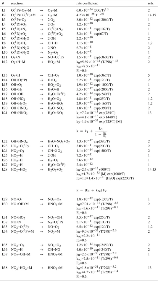
# reaction rate coefficient refs.
k1 O(3P)+O2+M → O3+M 6.0×10⁻³⁴(300/T)2.3 2
k2 O(3P)+O(3P)+M → O2+M 4.23×10⁻²⁸T−2.0 14,15
k3 O(3P)+O3 → 2 O2 8.0×10⁻¹²exp(-2060/T) 1
k4 O(1D)+O3 → 2 O2 1.2×10⁻¹⁰ 2
k5 O(1D)+N2 → O(3P)+N2 1.8×10⁻¹¹exp(107/T) 1
k6 O(1D)+O2 → O(3P)+O2 3.2×10⁻¹¹exp(67/T) 1
k7 O(1D)+H2O → 2 OH 2.2×10⁻¹⁰ 2
k8 O(1D)+H2 → OH+H 1.1×10⁻¹⁰ 1,2
k9 O(1D)+N2O → 2 NO 6.7×10⁻¹¹ 2
k10 O(1D)+N2O → N2+O2 4.4×10⁻¹¹ 1
k11 O2+N → NO+O(3P) 1.5×10⁻¹¹exp(-3600/T) 2
k12 O2+H+M → HO2+M k0=5.69×10⁻³²(T/298)−1.6
k∞=7.5×10⁻¹¹
Fc=0.6
2
k13 O3+H → OH+O2 1.0×10⁻¹⁰exp(-367/T) 5
k14 OH+O(3P) → H+O2 2.2×10⁻¹¹exp(120/T) 2
k15 OH+O3 → HO2+O2 1.9×10⁻¹²exp(-1000/T) 1
k16 OH+H2 → H2O+H 5.5×10⁻¹²exp(-2000/T) 2
k17 OH+OH → H2O+O(3P) 4.2×10⁻¹²exp(-240/T) 2
k18 OH+HO2 → H2O+O2 4.8×10⁻¹¹exp(250/T) 1,2
k19 OH+H2O2 → H2O+HO2 2.9×10⁻¹²exp(-160/T) 1,2
k20 OH+HNO2 → H2O+NO2 1.8×10⁻¹¹exp(-390/T) 2
k21 OH+HNO3 → H2O+NO3 k1=7.2×10⁻¹⁵exp(785/T)
k2=4.1×10⁻¹⁶exp(1440/T)
k3=1.9×10⁻³³exp(725/T) [M]
k = k1 +
k3
1 + k3 k2
13
k22 OH+HNO4 → H2O+NO2+O2 1.3×10⁻¹²exp(380/T) 2
k23 HO2+O(3P) → OH+O2 3.0×10⁻¹¹exp(200/T) 2
k24 HO2+O3 → OH+2 O2 1.1×10⁻¹⁴exp(-500/T) 2
k25 HO2+H → 2 OH 7.2×10⁻¹¹ 1
k26 HO2+H → H2+O2 5.6×10⁻¹² 1
k27 HO2+H → H2O+O(3P) 2.4×10⁻¹² 1
k28 HO2+HO2 → H2O2+O2 k0=2.3×10⁻¹³(600/T)
k∞=1.7×10⁻³³[M] exp(1000/T)
Fc=1.0+1.4×10⁻²¹[H2O] exp(2200/T)
k = (k0 + k∞)Fc
14,15
k29 NO+O3 → NO2+O2 1.8×10⁻¹²exp(-1370/T) 1
k30 NO+OH+M → HNO2+M k0=7.01×10⁻³¹(T/298)−2.6
k∞=3.6×10⁻¹¹(T/298)−0.1
Fc=0.6
2
k31 NO+HO2 → NO2+OH 3.5×10⁻¹²exp(250/T) 2
k32 NO+N → N2+O(3P) 2.1×10⁻¹¹exp(100/T) 2
k33 NO2+O(3P) → NO+O2 6.5×10⁻¹²exp(120/T) 1,2
k34 NO2+O(3P)+M → NO3+M k0=9.0×10⁻³²(T/298)−2.0
k∞=2.2×10⁻¹¹
Fc=0.6
2
k35 NO2+O3 → NO3+O2 1.2×10⁻¹³exp(-2450/T) 2
k36 NO2+H → OH+NO 4.0×10⁻¹⁰exp(-340/T) 2
k37 NO2+OH+M → HNO3+M k0=2.6×10⁻³⁰(T/298)−2.9
k∞=7.5×10⁻¹¹(T/298)−0.6
Fc=0.6
1
k38 NO2+HO2+M → HNO4+M k0=1.8×10⁻³¹(T/298)−3.2
k∞=4.7×10⁻¹²(T/298)−1.4
Fc=0.6
Table 4.Continued.
# reaction rate coefficient refs.
k39 HNO4+M → NO2+HO2+M k0=1.8×10⁻³¹(T/298)−3.2 k∞=4.7×10⁻¹²(T/298)−1.4
kinv=2.1×10⁻²⁷exp(10900/T) Fc=0.6
13
k40 NO2+NO3+M → N2O5+M k0=2.0×10⁻³⁰(T/298)−4.4
k∞=1.4×10⁻¹²(T/298)−0.7
Fc=0.6
14,15
k41 N2O5+M → NO2+NO3+M k0=2.0×10⁻³⁰(T/298)−4.4
k∞=1.4×10⁻¹²(T/298)−0.7
kinv=3.0×10⁻²⁷exp(10991/T)
Fc=0.6
14,15
k42 NO3+NO → 2NO2 1.8×10⁻¹¹exp(110/T) 1
k43 NO3+HO2 → 0.4HNO3+0.6 OH+0.6NO2 2.3×10⁻¹²exp(170/T) 6
k44 CH3CCl3+OH → H2O 1.8×10⁻¹²exp(-1550/T) 2
k45 CH4+OH → CH3O2+H2O 2.45×10⁻¹²exp(-1775/T) 2
k46 CH4+O(1D) → CH3O2+OH 2.25×10⁻¹⁰ 7
k47 CH4+O(1D) → CH2O+H2 1.65×10⁻¹¹ 1,2,8
k48 CH4+O(1D) → CH3OH 4.98×10⁻¹¹ 9
k49 CH3O2+NO → CH3O+NO2 3.0×10⁻¹²exp(280/T) 2
k50 CH3O2+NO3 → CH3O+NO2+O2 3.1×10⁻¹² 10
k51 CH3O2+HO2 → CH3OOH+O2 3.8×10⁻¹³exp(800/T) 1,2
k52 CH3O2+CH3O2 → CH3OH+CH2O+O2 1.5×10⁻¹³exp(190/T) 2,11
k53 CH3O2+CH3O2 → 2CH3O+O2 1.0×10⁻¹³exp(190/T) 2,11
k54 CH3O+O2 → CH2O+HO2 3.9×10⁻¹⁴exp(-900/T) 2
k55 CH3O+NO2 → CH2O+HNO2 1.1×10⁻¹¹exp(-1200/T) 2
k56 CH3OH+OH → CH2O+HO2+H2O 3.1×10⁻¹²exp(-360/T) 1
k57 CH3OOH+OH → CH2O+OH+H2O 1.0×10⁻¹²exp(190/T) 1
k58 CH3OOH+OH → CH3O2+H2O 1.9×10⁻¹²exp(190/T) 1
k59 CH2O+OH → CO+HO2+H2O 8.59×10⁻¹²exp(20/T) 1
k60 CH2O+NO3 → CO+HO2+HNO3 5.8×10⁻¹⁶ 1
k61 CH2O+O(3P) → CO+HO2+OH 3.4×10⁻¹¹exp(-1600/T) 2,12
k62 CO+OH → CO2+H 1.57×10⁻¹³+3.54×10⁻³³[M] 16
k63 C2H6+OH → C2H5O2+H2O 1.52×10⁻¹⁷exp(-498/T) T2 13 k64 C2H5O2+NO → CH3CHO+HO2+NO2 2.7×10⁻¹²exp(360/T) 13
k65 C2H5O2+NO3 → CH3CHO+HO2+NO2+O2 2.4×10⁻¹² 13
k66 C2H5O2+HO2 → C2H5OOH+O2 4.4×10⁻¹³exp(900/T) 13
k67 C2H5O2+CH3O2 → 0.74CH2O+0.74CH3CHO+
0.96HO2+0.26CH3OH+0.26C2H5OH
2.0×10⁻¹³ 13
k68 C2H5O2+C2H5O2 → 1.63CH3CHO+1.26HO2+
0.37C2H5OH
9.8×10⁻¹⁴exp(100/T) 13
k69 C2H5OOH+OH → C2H5O2+HO2 1.9×10⁻¹²exp(190/T) 13
k70 C2H5OOH+OH → CH3CHO+OH+H2O 7.69×10⁻¹⁷exp(253/T) T2 13
k71 C2H5OH+OH → CH3CHO+HO2+H2O 6.18×10⁻¹⁸exp(532/T) T2 13
k72 C3H8+OH → C3H7O2+H2O 1.55×10⁻¹⁷exp(-61/T) T2 13
k73 C3H7O2+NO → 0.72CH3COCH3+0.94NO2+ 0.22CH3CHO+0.94HO2+0.06ONITU
2.7×10⁻¹²exp(360/T) 13
k74 C3H7O2+NO3 → 0.234CH3CHO+NO2+HO2+ 0.766CH3COCH3
2.4×10⁻¹² 13
k75 C3H7O2+HO2 → C3H7OOH+O2 1.9×10⁻¹³exp(1300/T) 13
k76 C3H7O2+CH3O2 → 0.128CH3COCH3+0.78HO2+
0.695CH2O+0.305CH3OH+
0.567CH3CHO
5.18×10⁻¹² 13
k77 C3H7OOH+OH → C3H7O2+H2O 1.9×10⁻¹²exp(190/T) 13
k78 C3H7OOH+OH → CH3CHO+OH+H2O 1.67×10⁻¹⁷exp(253/T)T2 13
k79 CH3COCH3+OH → PROPAO2+H2O 2.81×10⁻¹²exp(-760/T) 1
k80 PROPAO2+NO → CH3CO3+CH2O+NO2 2.7×10⁻¹²exp(360/T) 13
k81 PROPAO2+NO3 → CH3CO3+CH2O+NO2+O2 2.4×10⁻¹² 13
k82 PROPAO2+HO2 → PROPAOOH+O2 1.9×10⁻¹³exp(1300/T) 13
k83 PROPAO2+CH3O2 → 1.31CH2O+0.23CH3OH+ 0.23CH3COCHO+0.54HO2+ 0.54CH3CO3
Table 4.Continued.
# reaction rate coefficient refs.
k84 PROPAOOH+OH → PROPAO2+H2O 1.9×10⁻¹²exp(190/T) 13
k85 PROPAOOH+OH → CH3COCHO+OH+H2O 4.69×10⁻¹⁷exp(253/T)T2 13
k86 C2H4+OH+M → 0.667PROPEO2+M k0=1.0×10⁻²⁸(T/298)−0.8
k∞=8.79×10⁻¹²
Fc=0.7
2
k87 C2H4+O3 → CH2O+0.46CO+0.16HO2+
0.08OH+0.17CO2
1.2×10⁻¹⁴exp(-2630/T) 2
k88 C3H6+OH+M → PROPEO2+M k0=2.94×10⁻²⁷(T/298)−3.0
k∞=2.775×10⁻¹¹(T/298)−1.3
Fc=0.5
13
k89 C3H6+O3 → 0.63248CH2O+0.341CH3O2+
0.0868CH4+0.4166CO+
0.0124CH3OH+0.2096HO2+
0.2474OH+0.38CH3CHO+0.2754CO2
6.51×10⁻¹⁵exp(-1900/T) 2
k90 PROPEO2+NO → CH3CHO+CH2O+HO2+NO2 2.7×10⁻¹²exp(360/T) 13
k91 PROPEO2+NO3 → CH3CHO+CH2O+ HO2+NO2+O2 2.4×10⁻¹² 13
k92 PROPEO2+HO2 → PROPEOOH+O2 1.9×10⁻¹³exp(1300/T) 13
k93 PROPEO2+CH3O2 → 0.305CH3OH+0.78HO2+
1.085CH2O+0.39CH3CHO+
0.305CH3COCHO
7.583×10⁻¹³ 13
k94 PROPEOOH+OH → PROPEO2+H2O 1.9×10⁻¹²exp(190/T) 13
k95 PROPEOOH+OH → CH3COCHO+OH+H2O 2.35×10⁻¹⁷exp(696/T)T2 13
k96 PROPEOOH+OH → CH3COCHO+OH+H2O 2.69×10⁻¹⁷exp(253/T)T2 13
k97 PROPEOOH+OH → CH3CHO+HO2+H2O 1.26×10⁻¹⁷exp(253/T)T2 13
k98 PROPEOOH+OH → PROPAOOH+HO2+H2O 3.19×10⁻¹⁸exp(696/T)T2 13
k99 CH3CHO+OH → CH3CO3+H2O 5.6×10⁻¹²exp(270/T) 2
k100 CH3CHO+NO3 → CH3CO3+HNO3 1.4×10⁻¹²exp(-1860/T) 13
k101 CH3CO3+NO → CH3O2+NO2+CO2 5.3×10⁻¹²exp(360/T) 13
k102 CH3CO3+NO2+M → PAN+M k0=2.7×10⁻²⁸(T/298)−7.1
k∞=1.2×10⁻¹¹(T/298)−0.9
Fc=0.3
13
k103 PAN+M → CH3CO3+NO2+M k0=5.0×10⁻²exp(-12875/T)
k∞=2.2×10+16exp(-13435/T)
Fc=0.27
13
k104 CH3CO3+NO3 → CH3O2+NO2+CO2+O2 5.0×10⁻¹² 13
k105 CH3CO3+HO2 → 0.3O3+0.3CH3OOH+
0.7O2+0.7CH3C(O)OOH
4.3×10⁻¹³exp(1040/T) 13
k106 CH3CO3+CH3O2 → CH2O+0.86CH3O2+
0.86HO2+0.86CO2+O2+
0.14CH3COOH
1.3×10⁻¹²exp(640/T) 13
k107 CH3CO3+CH3CO3 → 2CH3O2+2CO2 2.3×10⁻¹²exp(530/T) 13
k108 CH3C(O)OOH+OH → CH3CO3+H2O 1.9×10⁻¹²exp(190/T) 13
k109 C2H2+OH+M → 0.36CO+0.64CH3COCHO+
0.36HO2+0.65OH+M
k0=5.01×10⁻³⁰(T/298)−1.5
k∞=9.0×10⁻¹³(T/298)2.0
Fc=0.62
1
k110 ISOP+OH → ISOPO2 2.89×10⁻¹¹exp(335/T) 1,2
k111 ISOP+O3 → 0.42MACR+0.16MVK+
0.05C3H6+0.18OH+
0.09HO2+0.42CH2O+
0.27CO+0.07H2+0.15CO2
9.36×10⁻¹⁵exp(-1913/T) 13
k112 ISOP+NO3 → ISOPNO3 3.03×10⁻¹²exp(-446/T) 13
k113 ISOPO2+NO → 0.12ONITR+0.88NO2+
0.76HO2+0.608CH2O+
0.404MACR+0.354MVK+0.12XO2
2.7×10⁻¹²exp(360/T) 13
k114 ISOPO2+NO3 → 0.864HO2+NO2+0.69CH2O+
0.46MACR+0.403MVK+0.136XO2
2.4×10⁻¹² 13
k115 ISOPO2+HO2 → 0.867HO2+0.739CH2O+
0.506MACR+0.429MVK+ 0.133XO2+XOOH
Table 4.Continued.
# reaction rate coefficient refs.
k116 ISOPO2+CH3O2 → 0.305CH3OH+0.703HO2+
0.91CH2O+0.137XO2+
0.351MACR+0.205MVK
1.33×10⁻¹² 13
k117 ISOPO2+CH3CO3 → 0.275CH3COOH+0.58HO2+
0.725CO+0.725CH3O2+
0.198XO+20.397CH2O+
0.504MACR+0.296MVK
7.96×10⁻¹² 13
k118 ISOPNO3+NO → 1.206NO2+0.794HO2+
0.072CH2O+0.167MACR+
0.039MVK+0.794ONITR
2.7×10⁻¹²exp(360/T) 13
k119 ISOPNO3+NO3 → 1.206NO2+0.794HO2+
0.072CH2O+0.167MACR+
0.039MVK+0.794ONITR
2.4×10⁻¹² 13
k120 ISOPNO3+HO2 → 0.206NO2+0.794HO2+
0.008CH2O+0.167MACR+
0.039MVK+0.794ONITR+XOOH
1.9×10⁻¹³exp(1300/T) 13
k121 ISOPNO3+CH3O2 → 0.305CH3OH+0.711HO2+
0.697CH2O+0.06NO2+
0.059MACR+0.001MVK+ 0.635ONITR
1.749×10⁻¹² 13
k122 APIN+OH → APINO2 1.08×10⁻¹¹exp(444/T) 13
k123 APIN+O3 → 0.56OH+0.56APINO3 1.1615×10⁻¹⁵exp(-732/T) 13
k124 APIN+NO3 → APINO2+NO2 1.19×10⁻¹²exp(490/T) 13
k125 APINO2+NO → PCHO+NO2+HO2 2.7×10⁻¹²exp(360/T) 13
k126 APINO2+NO3 → PCHO+NO2+HO2+O2 2.4×10⁻¹² 13
k127 APINO2+HO2 → PCHO+HO2+XOOH 1.9×10⁻¹³exp(1300/T) 13
k128 APINO2+CH3O2 → 0.305CH3OH+0.695APINO3+HO2 1.22×10⁻¹³ 13
k129 APINO2+CH3CO3 → 0.725CO2+0.725CH3O2+
0.725PCHO+0.725HO2+
0.275CH3COOH
7.37×10⁻¹³ 13
k130 APINO3+NO → NO2+CO2+CH3COCH3+ 2PROPEO2 5.3×10⁻¹²exp(360/T) 13
k131 APINO3+NO2+M → APINPAN+M k0=2.7×10⁻²⁸(T/298)−7.1
k∞=1.2×10⁻¹¹(T/298)−0.9
Fc=0.3
13
k132 APINPAN+M → APINO3+NO2+M k0=4.0×10⁻³exp(-12100/T)
k∞=5.4×10+16exp(-13830/T)
Fc=0.3
14,15
k133 APINO3+NO3 → NO2+CO2+CH3COCH3+
2PROPEO2+O2
5.0×10⁻¹² 13
k134 APINO3+HO2 → 0.3O3+0.3CH3COOH+
0.7O2+0.7CH3C(O)OOH
4.3×10⁻¹³exp(1040/T) 13
k135 APINO3+CH3O2 → 0.335CH2O+0.665CH2O+
0.665HO2+0.665CH3COCH3+
1.33PROPEO2+CO2
4.52×10⁻¹² 13
k136 APINO3+CH3CO3 → 2CO2+CH3O2+
CH3COCH3+2PROPEO2
4.6×10⁻¹²exp(530/T) 13
k137 APINO3+APINO3 → 2CO2+2CH3COCH3+4PROPEO2 2.3×10⁻¹²exp(530/T) 13
k138 MACR+OH → 0.5MACRO2+0.5HO2+0.5MCO3 1.86×10⁻¹¹exp(175/T) 13
k139 MACR+O3 → 0.8CH3COCHO+0.13HO2+
0.37CO+0.1H2+0.2OH+
0.34CH2O+0.14CO2
1.359×10⁻¹⁵exp(-2112/T) 13
k140 MVK+OH → MACRO2 2.67×10⁻¹²exp(452/T) 13
k141 MVK+O3 → 0.05CH2O+0.95CH3COCHO+
0.08OH+0.15HO2+0.12H2+
0.16CO2+0.44CO
7.51×10⁻¹⁶exp(-1521/T) 13
k142 MACRO2+NO → 0.015ONITR+0.985NO2+
0.985HO2+0.158CH2O+
0.158CH3COCHO+0.828CO+
0.828CH3COCHO
Table 4.Continued.
# reaction rate coefficient refs.
k143 MACRO2+NO3 → NO2+HO2+0.16CH2O+
0.16CH3COCHO+0.84CO+
0.84CH3COCHO
2.4×10⁻¹² 13
k144 MACRO2+HO2 → MACROOH 1.9×10⁻¹³exp(1300/T) 13
k145 MACRO2+CH3O2 → 0.916HO2+1.064CH2O+
0.458CO+0.458CH3COCHO+
0.229CH3OH+0.458CH3CHO+
4.1288×10⁻¹³ 13
k146 MACRO2+CH3CO3 → 0.794CO2+0.794CH3O2+
0.412CH3CHO+0.544CH2O+
0.794CH3COCHO+0.794HO2+
0.206CH3COOH+0.25CO
2.475×10⁻¹² 13
k147 MACROOH+OH → MACRO2+H2O 1.9×10⁻¹²exp(190/T) 13
k148 MACROOH+OH → 2CH3CHO+OH+H2O 3.9×10⁻¹⁷exp(253/T)T2 13
k149 MACROOH+OH → MCO3+H2O 2.27×10⁻¹⁷exp(696/T)T2 13
k150 MACROOH+OH → 0.6C2H5OOH+HO2+
0.4CH3CHO+H2O
5.16×10⁻¹⁷exp(253/T)T2 13
k151 MCO3+NO → CH3CO3+CH2O+NO2 5.3×10⁻¹²exp(360/T) 13
k152 MCO3+NO2+M → MPAN+M k0=2.7×10⁻²⁸(T/298)−7.1
k∞=1.2×10⁻¹¹(T/298)−0.9
Fc=0.3
13
k153 MPAN+M → MCO3+NO2+M k0=5.0×10⁻²exp(-12875/T)
k∞=2.2×10+16exp(-13435/T)
Fc=0.27
13
k154 MCO3+NO3 → CH3CO3+CH2O+NO2+O2 5.0×10⁻¹² 13
k155 MCO3+HO2 → 0.3O3+0.3CH3COOH+
0.7O2+0.7CH3C(O)OOH
4.3×10⁻¹³exp(1040/T) 13
k156 MCO3+CH3O2 → 1.655CH2O+0.665HO2+
0.665CH3CO3+0.665CO2
4.52×10⁻¹² 13
k157 MCO3+CH3CO3 → 2CO2+CH3O2+CH2O+CH3CO3 4.6×10⁻¹²exp(530/T) 13
k158 MCO3+MCO3 → 2CO2+2CH3O2+ 2CH2O+2CH3CO3 2.3×10⁻¹²exp(530/T) 13
k159 CH3COCHO+OH → CH3CO3+CO+H2O 8.4×10⁻¹³exp(830/T) 17
k160 CH3COCHO+NO3 → CH3CO3+CO+HNO3 1.4×10⁻¹²exp(-1860/T) 13
k161 PCHO+OH → PCO3+H2O 9.1×10⁻¹¹ 13
k162 PCHO+NO3 → PCO3+HNO3 5.4×10⁻¹⁴ 13
k163 PCO3+NO → PROPEO2+NO2+CO2+XO2 5.3×10⁻¹²exp(360/T) 13
k164 PCO3+NO2+M → PCO3PAN+M k0=2.7×10⁻²⁸(T/298)−7.1
k∞=1.2×10⁻¹¹(T/298)−0.9
Fc=0.3
13
k165 PCO3PAN+M → PCO3+NO2+M k0=5.0×10⁻²exp(-12875/T)
k∞=2.2×10+16exp(-13435/T)
Fc=0.27
13
k166 PCO3+NO3 → PROPEO2+NO2+CO2+XO2 5.0×10⁻¹² 13
k167 PCO3+HO2 → 0.3O3+0.3CH3COOH+
0.7O2+0.7CH3C(O)OOH
4.3×10⁻¹³exp(1040/T) 13
k168 PCO3+CH3O2 → 0.665PROPEO2+CH2O+
0.665HO2+0.665XO2
4.52×10⁻¹² 13
k169 PCO3+CH3CO3 → 2CO2+PROPEO2+XO2+CH3O2 4.6×10⁻¹²exp(530/T) 13
k170 PCO3+PCO3 → 2CO2+2PROPEO2+2XO2 2.3×10⁻¹²exp(530/T) 13
k171 ONITU+OH → 0.694ONITUO2+0.25HNO3+
0.25HO2+0.3CH3COCH3+0.05NO2
1.83×10⁻¹² 13
k172 ONITUO2+NO → 1.294NO2+0.706ONITR+
0.4HO2+0.116CH2O+
0.386CH3CHO+0.209MEK+
0.395XO2
2.7×10⁻¹²exp(360/T) 13
k173 ONITUO2+NO3 → 1.294NO2+0.706ONITR+
0.4HO2+0.116CH2O+
0.386CH3CHO+0.209MEK+
0.395XO2
2.4×10⁻¹² 13
k174 ONITUO2+HO2 → 0.7ONITR+0.3ONITUO2 1.9×10⁻¹³exp(1300/T) 13
Table 4.Continued.
# reaction rate coefficient refs.
k176 ONITR+NO3 → MCO3+0.4HNO3+0.8NO2+0.8NO 1.4×10⁻¹²exp(-1860/T) 13
k177 MEK+OH → MEKO2 3.24×10⁻¹⁸exp(414/T)T2 13
k178 MEKO2+NO → NO2+1.329CH3CHO+
0.6CH3CO3+0.07CH2O+
0.4HO2+0.197MEK
2.7×10⁻¹²exp(360/T) 13
k179 MEKO2+NO3 → NO2+1.329CH3CHO+
0.6CH3CO3+0.07CH2O+
0.4HO2+0.197MEK
2.4×10⁻¹² 13
k180 MEKO2+HO2 → MEKOOH 1.9×10⁻¹³exp(1300/T) 13
k181 MEKO2+CH3O2 → 0.305CH3OH+0.699HO2+
0.75CH2O+0.08CH3CO3+
0.295MEK+0.654CH3CHO+
0.042CH3COCHO
9.764×10⁻¹³ 13
k182 MEKOOH+OH → MEKO2+H2O 1.9×10⁻¹²exp(190/T) 13
k183 MEKOOH+OH → MEK+ OH+H2O 1.17×10⁻¹⁷exp(696/T)T2 13
k184 MEKOOH+OH → CH3CHO+0.5MEK+OH+H2O 9.75×10⁻¹⁷exp(253/T)T2 13
k185 MEKOOH+OH → CH3COCHO+OH+H2O 3.28×10⁻¹⁸exp(253/T)T2 13
k186 ALKEN+OH → ALKENO2 9.19×10⁻¹²exp(-522.22/T) 13
k187 ALKEN+O3 → 0.9CH3CHO+0.23ALKENO2+
0.09CH3COCH3+0.34CH3O2+
0.08CH4+0.02C2H6+0.3CO+
0.01CH3OH+0.42OH
4.95×10⁻¹⁵exp(-1054.84/T) 13
k188 ALKEN+NO3 → ALKENO2+NO2 3.95×10⁻¹²exp(-327.93/T) 13
k189 ALKENO2+NO → 0.034ONITU+0.406CH2O+
1.666CH3CHO+0.966NO2+
0.38CH3COCH3+0.966HO2
2.7×10⁻¹²exp(360/T) 13
k190 ALKENO2+NO3 → 0.393CH3COCH3+NO2+HO2+
0.724CH3CHO+0.42CH2O
2.4×10⁻¹² 13
k191 ALKENO2+HO2 → ALKENOOH 1.9×10⁻¹³exp(1300/T) 13
k192 ALKENO2+CH3O2 → 0.305CH3OH+0.265CH3CHO+
0.695CH2O+0.06CH3COCH3+
0.305CH3COCHO+0.78HO2
1.22×10⁻¹³ 13
k193 ALKENOOH+OH → ALKENO2+H2O 1.9×10⁻¹²exp(190/T) 13
k194 ALKENOOH+OH → CH3COCHO+OH+H2O 9.46×10⁻¹⁷exp(253/T)T2 13
k195 ALKAN+OH → ALKANO2 1.63×10⁻¹⁷exp(385.22/T)T2 13
k196 ALKANO2+NO → 0.007CH2O+0.362CH3CHO+
0.289CH3COCH3+0.799NO2+
0.412MEK+0.082CH3O2+
0.2ONITU+0.268XO2+ 0.449HO2
2.7×10⁻¹²exp(260/T) 13
k197 ALKANO2+NO3 → NO2+0.562HO2+0.336XO2+
0.101CH3O2+0.517MEK+
0.001CH2O+0.454CH3CHO
2.4×10⁻¹² 13
k198 ALKANO2+HO2 → ALKANOOH 1.9×10⁻¹³exp(1300/T) 13
k199 ALKANO2+CH3O2 → 0.045CH3COCH3+0.626HO2+
0.305CH3OH+0.696CH2O+
0.315MEK+0.012CH3O2+
0.442CH3CHO+0.14XO2
3.7652×10⁻¹³ 13
k200 ALKANOOH+OH → ALKANO2+H2O 1.9×10⁻¹²exp(190/T) 13
k201 ALKANOOH+OH → CH3CHO+OH+H2O 1.07×10⁻¹⁷exp(253/T)T2 13
k202 ALKANOOH+OH → MEK+OH+H2O 3.82×10⁻¹⁷exp(696/T)T2 13
k203 AROM+OH → 0.77AROMO2+0.212HO2 1.01×10⁻¹¹exp(58.45/T) 13
k204 AROMO2+NO → 0.423CH3COCHO+NO2+
0.658CH3CO3+0.658CO+1.658HO2
2.7×10⁻¹²exp(360/T) 13
k205 AROMO2+NO3 → 0.423CH3COCHO+NO2+
0.658CH3CO3+0.658CO+1.658HO2
2.4×10⁻¹² 13
k206 AROMO2+HO2 → AROMOOH 1.9×10⁻¹³*exp(1300/T) 13
k207 AROMO2+CH3O2 → 0.087*CH3COCHO + 0.135*CO+
0.135*CH3CO3 + 0.305*CH3OH+
0.695*CH2O + 0.915*HO2
2.31×10⁻¹³ 13
Table 4.Continued.
# reaction rate coefficient refs.
k209 AROMOOH+OH → OH+H2O 4.61×10⁻¹⁸exp(253/T)T2 13
k210 AROMOOH+OH → CH3CO3+CO+OH+ HO2+H2O 4.19×10⁻¹⁷exp(696/T)T2 13
k211 XO2+NO → NO2+HO2 2.7×10⁻¹²exp(360/T) 13
k212 XO2+NO3 → NO2+HO2 2.4×10⁻¹² 13
k213 XO2+HO2 → XOOH 1.9×10⁻¹³exp(1300/T) 13
k214 XO2+CH3O2 → 0.305CH3O2+0.695CH2O+0.39HO2 1.22×10⁻¹³ 13
k215 XO2+CH3CO3 → 0.275CH3COOH+0.725CO2+
0.725CH3O2
7.37×10⁻¹³ 13
k216 XOOH+OH → XO2+H2O 1.9×10⁻¹²exp(190/T) 13
k217 XOOH+OH → OH+H2O 7.69×10⁻¹⁷exp(253/T)T2 13
T=temperature (K); M=air density (molecules cm−3)
Rate coefficients are in cm3molecules−1s−1for bimolecular reactions and in cm6molecules−2s−1for termolecular reactions.
In the latter case, the rate coefficient is defined by
k(T,M)=
k0(T)· [M]
1+k0(T)· [M]
k∞(T)
·Fc (
1+
log10 k
0(T)· [M]
k∞(T) 2)−1
References:
1, Atkinson et al. (1997); 2, DeMore et al. (1997); 3, Jenkin and Cox (1987); 4, Matzkies and Manthe (1998) 5, Yu and Varandas (1997); 6, Hall et al. (1988); 7, Matsumi et al. (1993); 8, Greenberg and Heicklen (1972) 9, Bradley et al. (1971); 10, Kukui et al. (1995); 11, Tyndall et al. (1998); 12, Baulch et al. (1992)
The LMDz version used in this study (referred to as 3.3) has a horizontal resolution of 3.8 degrees in longitude and 2.5 degrees in latitude (96×72 grid cells). The model is composed of 19 vertical levels onσ-p coordinates extending from the surface to 3 hPa. Also higher-resolution versions of LMDz have been developed and applied recently (e.g. Bauer et al., 2004).
The primitive equations in the GCM are solved with a 3 min time-step, large-scale transport of tracers is carried out every 15 min, and physical processes are calculated at a 30 min time interval. For a more detailed description and an extended evaluation of the GCM we refer to the work of, e.g., Le Treut et al. (1994) and Harzallah and Sadourny (1995). Recently, Hauglustaine et al. (2004) have coupled LMDz to the tropospheric chemistry model INCA, during which the GCM has been reevaluated.
2.2 The INCA-NMHC chemistry and aerosol model
INteraction withChemistry andAerosols (INCA) is coupled on-line to the LMDz general circulation model. INCA pre-pares the surface and in situ emissions, calculates dry de-position and wet scavenging rates, and integrates in time the concentration of atmospheric species with a time step of 30 min. INCA uses a sequential operator approach, a method generally applied in chemistry-transport-models (Muller and Brasseur, 1995; Brasseur et al., 1998; Wang et al., 1998a; Poisson et al., 2000). The INCA-NMHC version applied in this study is based on an earlier version which was de-veloped to represent the background chemistry of the tropo-sphere (Hauglustaine et al., 2004). Results from this version of the model related to the impact of chemistry on the budget of CO2have been published by Folberth et al. (2005).
2.2.1 Chemistry
The version of INCA used in this study includes a compre-hensive photochemical scheme originally intended to repre-sent the photochemistry of the troposphere in regional scale chemistry-transport models. In addition to the CH4–NOx–
CO–O3 photochemistry representative of the tropospheric
background, INCA, in its NMHC-implementation, also takes into account the photochemical oxidation pathways of non-methane hydrocarbons (NMHC) and non-non-methane volatile organic compounds (NMVOC) from natural and anthro-pogenic sources as well as their photochemical oxidation products. The model can be applied to calculate the distri-bution of tropospheric ozone and its precursors, but due to the comprehensive chemistry scheme the model is also suited to be used in studies of biosphere-atmosphere interrelation and the impact of a changing biosphere on the global cli-mate. The species included in this more extensive version of LMDz-INCA are summarized in Tab. 1. We consider only one photochemical family (Ox=O3+O(1D)+O(3P)), and
for species with very short photochemical lifetimes transport is not taken into account.
Tables 1, 2, 3, and 4 summarize the chemical scheme in LMDz-INCA. The scheme includes a total of 83 species, 58 of which are subject to transport. In INCA-NMHC short-chained NMVOC are treated explicitly whereas a lump-ing approach is applied in the case of higher NMVOC as proposed by Brocheton (1999). Alkanes up to three car-bon atoms (C3) per molecule are treated explicitly including
methane, ethane, and propane. All C4- and higher alkanes
are lumped into one artificial species (C+4-alkanes). Like-wise, the model distinguishes ethene, propene, and C+4 -alkenes. The isoprene oxidation pathway has been repre-sented with some complexity, comparable to the one pro-posed by P¨oschl et al. (2000) including explicitly the ma-jor oxidation products methyl vinyl ketone and methacrolein; all higher isoprenoid species are lumped into one group to which we refer to as “terpenes”. INCA-NMHC includes two alcohols (methanol and C+2-alcohols, eleven hydroper-oxides, one group representing organic acids, three aldehyde species (formaldehyde, acetaldehyde including higher mono-carboxy aldehydes, and a group representing higher aldehy-des produced by terpene oxidation), three ketones (acetone, methyl ethyl ketone, and methyl vinyl ketone), four species representing peroxy acetyl nitrate (PAN) and analogues, two general organic nitrate groups (organic nitrates with low or high reactivity toward OH), as well as the corresponding or-ganic radicals arising in the oxidation of the above species (cf. Tables 1 and 4). Lumping in all cases follows the gen-erally applied method of grouping individual compounds by their reactivity toward the OH-radical while also taking into account compound groups, molecular weights, and atmo-spheric abundances (for a general description of these meth-ods see, e.g., Stockwell et al., 1997).
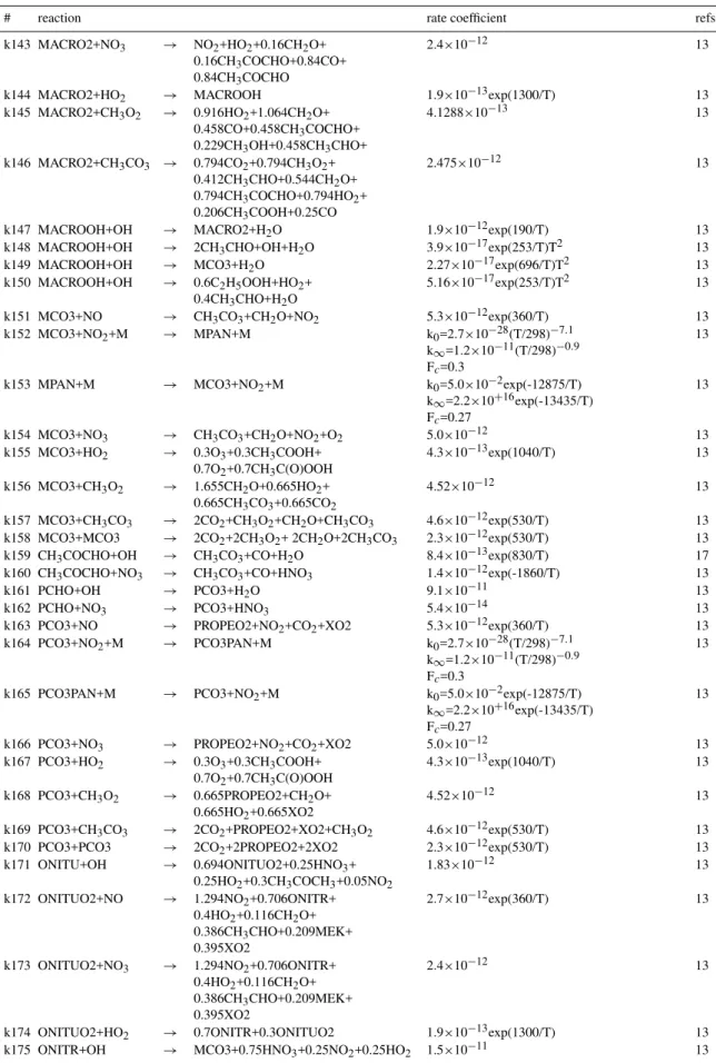
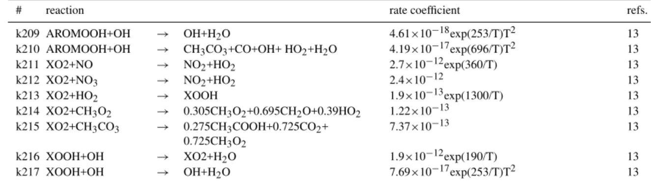
43 photolytic reactions (Table 2), 217 thermochemical re-actions (Table 4), and 4 heterogeneous rere-actions (Table 3) are taken into account by the model. The set of reactions and re-action rates is based on the scheme of Brocheton (1999). All reaction rates have been reviewed and updated with respect to the compilations of Atkinson et al. (1997) and DeMore et al. (1997) as well as subsequent updates (Sander et al., 2000, 2002). The reaction rates are calculated by the model at each time interval on the basis of temperature, pressure, and water vapour distribution provided by the GCM.
Hauglustaine et al. (2004). Where no spectral data is avail-able for a specific species to be used with TUV we as-sume the photolysis frequencies to be linearly dependent on chemically similar compounds (cf. Table 2). The LMDz-INCA chemical scheme includes four heterogeneous reac-tions (Table 3) following the recommendareac-tions of Jacob (2000) and using the monthly averaged sulfate aerosol fields from Boucher et al. (2002) to determine the aerosol distribu-tion as discussed by Hauglustaine et al. (2004). The NMHC-version of LMDz-INCA uses the identical parameterization for the representation of these processes.
The mechanism implicitly accounts for a carbon loss through formation of secondary organic aerosols (SOA). This tropospheric carbon sink is taken into account in the scheme as a carbon imbalance for specific reactions in the terpene oxidation pathway. The estimate of the global carbon sink as derived with LMDz-INCA amounts to approximately 39% (∼37 Tg C yr−1) of the total annual carbon surface flux
emit-ted as terpenes. Our estimate seems in satisfactory agreement with the calculated variation of the global annual SOA pro-duction of 2.5 to 44 Tg C yr−1for the biogenically produced SOA (Tsigaridis and Kanakidou, 2003). Note that explicit secondary organic aerosol formation is not calculated in the current implementation of LMDz-INCA and SOA are not in-cluded in the INCA species inventory.
Interactive calculation of chemistry and transport of species extends up to the upper model level. However, in the current version of INCA no chlorine or bromine chem-istry is taken into account and heterogeneous reactions on po-lar stratospheric clouds (PCS) is not yet considered. There-fore, ozone concentrations are relaxed toward observations at the uppermost model levels at each time step applying a relaxation time constant of ten days above the 380K poten-tial temperature surface. The ozone observations are taken from the monthly mean 3-D climatologies of Li and Shine (1995). Further details and an evaluation of the stratospheric boundary conditions in INCA can be found in Hauglustaine et al. (2004); the NMHC version of INCA applies the same approach.
Forward integration in time of the chemical equations is conducted on the basis of five possible numerical algorithms with a time step of 30 minutes as described by Hauglustaine et al. (2004). In the current configuration of LMDz-INCA we apply the explicit Euler forward algorithm (Brasseur et al., 1999) for the integration of long-lived species (marked “l” in Table 1) and the implicit Euler backward with Newton-Raphson iteration scheme for all other species (marked “s” in Table 1). A species to be long-lived in the above sense and suitable for the less resourceful numerical algorithm requires the mean atmospheric lifetime of this species to be at least a few weeks.
2.2.2 Emissions
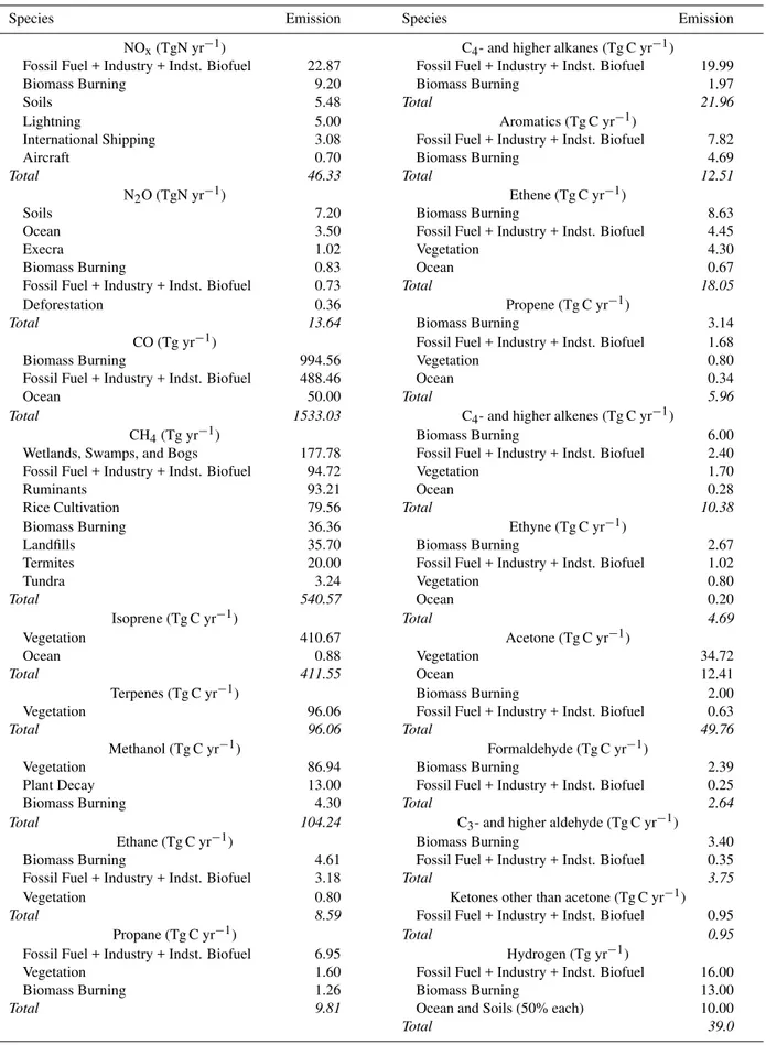
Surface emission inventories have been compiled for this ver-sion of LMDz-INCA using the same methods of data prepa-ration as described in Hauglustaine et al. (2004). These in-ventories are based on various compilations, with the excep-tion of the biogenic surface source. Biogenic surface emis-sions were prepared using a global vegetation model which includes a biogenic emission module. Table 5 summarizes the emission magnitude for the individual species that are considered in the version of LMDz-INCA and used in the current study.
LMDz-INCA uses anthropogenic emissions (industry, fos-sil fuel, and industrial biofuel) based on the EDGAR v3.2 and EDGAR v2.0 emission databases. Anthropogenic sources for nitrogen oxides (NOx), carbon monoxide (CO),
and methane (CH4) are introduced on the basis of the
es-timates provided in EDGAR v3.2 (Olivier and Berdowski, 2001) representative of the year 1995. The CO global emis-sions are rescaled to the values given by Prather et al. (2001). In addition, the LMDz-INCA emission inventory also in-cludes NOxemissions from oceangoing ships based on
Cor-bett et al. (1999) and NOx aircraft emissions based on the
ANCAT/EC2 inventory (Gardner et al., 1998).
At the time of creation of the current LMDz-INCA emis-sion inventory the more recent veremis-sion EDGAR v3.2 did not yet include NMVOC emissions on a per-compound ba-sis. Therefore, it was decided to use anthropogenic NMVOC emission estimates as given by the EDGAR v2.0 database (Olivier et al., 1996) which includes estimates for individual compounds. NMVOC emissions based on EDGAR v2.0 are representative of the year 1990 and include alkanes (C2H6,
C3H8, C+4-alkanes), alkenes and alkynes (C2H4, C3H6, C+4
-alkenes, C2H2), aromatics, aldehydes (CH2O, CH3CHO
plus higher aldehydes) as well as ketones (CH3COCH3and
higher ketones, methylethyl ketone, methylvinyl ketone). Species explicitly included in EDGAR v2.0 that are not ex-plicit in LMDz-INCA were aggregated into the specific com-pound group based on their individual molecular weights, their reactivity towards the hydroxyl radical, and their rel-ative atmospheric abundances.
Biomass burning emissions are introduced according to the satellite based inventory developed by Van der Werf et al. (2003), averaged over the period 1997–2001. This data set is used to provide the geographical distribution and sea-sonal variation for each compound. Domestic biofuel use and agricultural waste burning emissions are also included in the biomass burning category and are based on the EDGAR database. Emission factors compiled by Andreae and Merlet (2001) are then used to derive the emission magnitude of the biomass burning surface flux for the individual compounds.
NO soil emissions are introduced on the basis of Yienger and Levy II (1995), emissions of CH4from rice paddies,
Table 5.Global Surface Emissions of Trace Gases in LMDz-INCA.
Species Emission Species Emission
NOx(TgN yr−1) C4- and higher alkanes (Tg C yr−1)
Fossil Fuel + Industry + Indst. Biofuel 22.87 Fossil Fuel + Industry + Indst. Biofuel 19.99
Biomass Burning 9.20 Biomass Burning 1.97
Soils 5.48 Total 21.96
Lightning 5.00 Aromatics (Tg C yr−1)
International Shipping 3.08 Fossil Fuel + Industry + Indst. Biofuel 7.82
Aircraft 0.70 Biomass Burning 4.69
Total 46.33 Total 12.51
N2O (TgN yr−1) Ethene (Tg C yr−1)
Soils 7.20 Biomass Burning 8.63
Ocean 3.50 Fossil Fuel + Industry + Indst. Biofuel 4.45
Execra 1.02 Vegetation 4.30
Biomass Burning 0.83 Ocean 0.67
Fossil Fuel + Industry + Indst. Biofuel 0.73 Total 18.05
Deforestation 0.36 Propene (Tg C yr−1)
Total 13.64 Biomass Burning 3.14
CO (Tg yr−1) Fossil Fuel + Industry + Indst. Biofuel 1.68
Biomass Burning 994.56 Vegetation 0.80
Fossil Fuel + Industry + Indst. Biofuel 488.46 Ocean 0.34
Ocean 50.00 Total 5.96
Total 1533.03 C4- and higher alkenes (Tg C yr−1)
CH4(Tg yr−1) Biomass Burning 6.00
Wetlands, Swamps, and Bogs 177.78 Fossil Fuel + Industry + Indst. Biofuel 2.40 Fossil Fuel + Industry + Indst. Biofuel 94.72 Vegetation 1.70
Ruminants 93.21 Ocean 0.28
Rice Cultivation 79.56 Total 10.38
Biomass Burning 36.36 Ethyne (Tg C yr−1)
Landfills 35.70 Biomass Burning 2.67
Termites 20.00 Fossil Fuel + Industry + Indst. Biofuel 1.02
Tundra 3.24 Vegetation 0.80
Total 540.57 Ocean 0.20
Isoprene (Tg C yr−1) Total 4.69
Vegetation 410.67 Acetone (Tg C yr−1)
Ocean 0.88 Vegetation 34.72
Total 411.55 Ocean 12.41
Terpenes (Tg C yr−1) Biomass Burning 2.00
Vegetation 96.06 Fossil Fuel + Industry + Indst. Biofuel 0.63
Total 96.06 Total 49.76
Methanol (Tg C yr−1) Formaldehyde (Tg C yr−1)
Vegetation 86.94 Biomass Burning 2.39
Plant Decay 13.00 Fossil Fuel + Industry + Indst. Biofuel 0.25
Biomass Burning 4.30 Total 2.64
Total 104.24 C3- and higher aldehyde (Tg C yr−1)
Ethane (Tg C yr−1) Biomass Burning 3.40
Biomass Burning 4.61 Fossil Fuel + Industry + Indst. Biofuel 0.35 Fossil Fuel + Industry + Indst. Biofuel 3.18 Total 3.75
Vegetation 0.80 Ketones other than acetone (Tg C yr−1)
Total 8.59 Fossil Fuel + Industry + Indst. Biofuel 0.95
Propane (Tg C yr−1) Total 0.95
Fossil Fuel + Industry + Indst. Biofuel 6.95 Hydrogen (Tg yr−1)
Vegetation 1.60 Fossil Fuel + Industry + Indst. Biofuel 16.00
Biomass Burning 1.26 Biomass Burning 13.00
Total 9.81 Ocean and Soils (50% each) 10.00
are based on Bouwman and Taylor (1996) and Kroeze et al. (1999) for continental emissions and on Nevison and Weiss (1995) for the oceanic N2O surface flux. NO emissions from
lightning are calculated interactively in LMDz-INCA on the basis of the occurrence of convection and cloud top heights. The parameterization of NO from lightning sources as it is used in LMDz-INCA is discussed in more detail by Jourdain and Hauglustaine (2001) and Hauglustaine et al. (2004).
Biogenic emissions of isoprene, terpenes, methanol, and acetone have been prepared with the dynamical global vegetation model ORCHIDEE (Organizing Carbon and
Hydrology inDynamicEcosystEms) (Krinner et al., 2005). ORCHIDEE essentially includes three different components, namely the surface-vegetation-atmosphere transfer scheme SECHIBA (Ducoudr´e-De Noblet et al., 1993; de Rosnay and Polcher, 1998), the dynamic global vegetation model LPJ (Sitch et al., 2003), and STOMATE (Saclay-Toulouse-Orsay
Model for theAnalysis ofTerrestrialEcosystems), a newly developed model simulating plant phenology and carbon dy-namics. For a detailed description and extended evaluation of ORCHIDEE and the new carbon dynamics model STOM-ATE we refer to the paper by Krinner et al. (2005).
In order to calculate NMVOC surface fluxes from the ter-restrial biosphere, a biogenic emission module has recently been integrated into ORCHIDEE. The calculation is based on the emission model by Guenther et al. (1995) and uses input from ORCHIDEE for the key parameters (leaf area in-dex, PFT distribution, specific leaf weight, etc.). This model takes into account changes in the flux strength due to leaf temperature, photosynthetically active radiation (direct and diffuse), and leaf ageing. A detailed description and evalu-ation of the terrestrial NMVOC emission model is given by Lathi`ere et al..
Warneke et al. (1999) first suggested a significant source of methanol from decaying plant matter and recent esti-mates of its magnitude range between 4 and 17 Tg C yr−1 (Singh et al., 2000; Heikes et al., 2002; Galbally and Kirstine, 2002). The LMDZ-INCA emission inventory includes bio-genic methanol emissions deriving from plant decay with a global source strength of 13 Tg C yr−1. It is assumed that this methanol source collocates with methanol emissions from the terrestrial vegetation.
LMDz-INCA takes into account oceanic emissions of CO and several NMVOC (cf. Tab. 5 for compounds that pos-sess oceanic sources). The spatial distribution and variation in time of oceanic CO emissions is based on Erickson and Taylor (1992) and scaled to a global mean of 50 Tg C yr−1
(Prather et al., 2001). It was furthermore assumed that the global geographic distribution of oceanic NMVOC emis-sions equals the global oceanic CO source distribution. The oceanic NMVOC emission magnitude is based on Jacob et al. (2002) in case of acetone and on the work of Bonsang et al. (1992) and Bonsang and Boissard (1999) for all other NMVOC that posses non-zero oceanic sources in the LMDz-INCA emission inventory.
2.3 Dry deposition and wet removal
Dry deposition in LMDz-INCA is based on the resistance-in-series approach (Wesely, 1989; Walmsley and Wesely, 1996; Wesely and Hicks, 2000). Deposition velocities (vd) are cal-culated at each time step according to:
vd =
1
Ra+Rb+Rc
, (1)
where Ra, Rb, and Rc (s/m) are the aerodynamic, quasi-laminar, and surface resistance, respectively. RaandRbare determined on the basis of Walcek et al. (1986). The sur-face resistance calculation for all species included in LMDz-INCA is based on their temperature dependent Henry’s Law Equilibrium Constant and reactivity factor for the oxidation of biological substances. Henry’s Law Coefficients tabu-lated for standard conditions have been taken from Sander (1999) and reactivity factors are taken from Wesely (1989) and Walmsley and Wesely (1996). The vegetation map clas-sification of De Fries and Townshend (1994), interpolated to the model grid and redistributed into the classification of We-sely (1989), is used to parameterize land use dependencies of the surface resistanceRc. A complete list of species that are subject to dry deposition is given in Table 1. During the tran-sition from LMDz-INCA-CH4to LMDz-INCA-NMHC the
parameterization of dry deposition in the model has under-gone some revision taking into account recent work (see cf., e.g., Ganzeveld et al., 1998; Wesely and Hicks, 2000).
Wet scavenging in INCA is parameterized as a first-order loss process as proposed by Giorgi and Chameides (1985):
d
dtCg= −βCg, (2)
whereCg is the gas-phase concentration of the considered species andβ is the scavenging coefficient (1/s). Wet scav-enging associated with large scale stratiform precipitation is calculated adopting the falling raindrop approach (Seinfeld and Pandis, 1998) and wet removal of soluble species by convective precipitation is calculated as part of the upward convective mass flux on the basis of a modified version of the scheme proposed by Balkanski et al. (1993). INCA cal-culates wet scavenging of soluble species for convective and stratiform precipitation separately. Nitric acid is used as a reference and the scavenging rate of any other species sub-ject to wet removal is scaled to the scavenging rate of HNO3
3 Model evaluation
We present here a general evaluation of the LMDz-INCA model in its NMHC version using a simulation which is rep-resentative of the 1990s. During development the model has been run almost consecutively for more than 20 model years before a spin-up run for this study was initialized. A six months spin-up was then conducted from July to December using the restart files of the last development run. After this spin-up period the model has been run for another 24 con-secutive months, the last 12 months have been used in the analysis. This approach was chosen to ensure that even long-lived species such as methane have reached equilibrium.
The large amount of species considered in this model and the still rather sparse observational data available from mea-surement campaigns only allow us to discuss the major as-pects of global tropospheric chemistry in this evaluation of the model performance. Although the spatial distribution and time evolution of more than 80 species are calculated by LMDz-INCA, the discussion shall be focused on the key species and selected NMVOC. CO concentrations are eval-uated by comparison with surface climatologies from Nov-elli et al. (2003), other species simulated by LMDz-INCA including hydrocarbons, acetone, NOx, PAN, and HNO3
are compared to observations from various aircraft missions based on the data compilation by Emmons et al. (2000) and references therein. Finally, calculated ozone concentrations are evaluated by comparison with climatological ozonesonde observations (Logan, 1999).
3.1 Carbon monoxide
Direct surface emission deriving from fossil fuel combus-tion as well as biomass burning are the most important CO sources in the atmosphere. In addition, carbon monoxide is produced in situ by oxidation of methane and non-methane hydrocarbons in the entire troposphere.
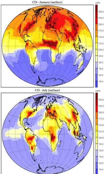
Figure 1 shows the monthly mean carbon monoxide sur-face mixing ratio for January and July. CO is most abun-dant near the surface sources of the tropics and the north-ern midlatitudes as well as during the northnorth-ern hemispheric winter when its photochemical lifetime is increased owing to a decrease in the OH abundance and weak vertical mixing. Predicted mixing ratios reach 300 ppb over these regions. During the summer months CO concentrations decrease sig-nificantly in the photochemically more active atmosphere, mostly due to a strong increase in OH.
In the tropics the seasonal cycle of CO is controlled to a large extent by the seasonality of biomass burning, which account for half of the direct CO emissions. Biomass burn-ing is most intense durburn-ing the dry season (December–April in the northern tropics, July – October in the southern trop-ics). Over these areas with intense biomass burning (tropical regions of Africa and South America) the model calculates maximum mixing ratios in the range of 200 to 300 ppb. In
Fig. 1.Carbon monoxide surface mixing ratio for January and July
(ppbv).
the marine boundary layer of the southern hemisphere, back-ground CO concentrations as predicted by LMDz-INCA are generally lower than 70 ppb.
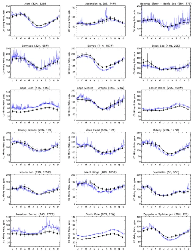
Simulated monthly mean carbon monoxide concentrations near the surface are compared with climatologies from ob-servations for 18 selected stations from the CMDL network (Novelli et al., 2003) in Fig. 2. Measurements are depicted as monthly means including their standard deviation over the period of record (5 to 10 years, depending on the station).
both in terms of seasonality and magnitude. The model also shows a good agreement with tropical sites in the northern hemisphere (e.g., Easter Islands, Canary Islands, Midway). The model reproduces the seasonal cycle and spring maxi-mum in the southern tropics (Ascension Island and Ameri-can Samoa) fairly well, which is governed by the seasonal biomass burning emissions (July to October in the southern hemisphere). However, the peak in CO is one month early at Ascension and overestimated but in phase at the Samoa site. The comparison suggests that the model is capable of re-producing CO concentration well at locations where well constrained anthropogenic CO sources contribute a signifi-cant portion of the emissions (practically all of the northern hemisphere). In the southern hemisphere, where CO concen-trations are generally lower and are dominated by biomass burning and, to some extent at southern high latitudes, even by the oceanic source, the model has a tendency of overesti-mating CO concentrations. This is most likely due to the CO biomass burning emission set, but could also be caused by an overestimate of the VOC emissions with subsequent in-situ formation of CO by photooxidation or an underestimate of the concentration of hydroxyl radicals near the surface at these locations. In general though, the tendency to underes-timate CO concentrations, persistent in many current chem-istry models both taking and not taking into account VOC photochemistry (cf., e.g., Hauglustaine et al., 1998; Poisson et al., 2000; Bey et al., 2001; Hauglustaine et al., 2004), is not discernible in the NMHC version of LMDz-INCA, which we tentatively attribute to the spatial and time variability of the OH abundance well reproduced by the model (cf. Sect. 3.2). 3.2 Hydroxyl radical and methane concentration
OH is most abundant in the tropical lower and mid troposphere reflecting high levels of ultraviolet radiation and water vapour. OH concentrations can reach 20 to 30×105molecules cm−3in this atmospheric domain and de-crease with altitude due to a decline in water vapour abun-dance.
The global mean OH concentration as calculated by the model can be evaluated by using the methylchloro-form (CH3CCl3) lifetime as a proxy (Spivakovsky et al.,
1990; Prinn et al., 1995). Spivakovsky et al. (2000) cal-culated a global mean atmospheric lifetime of 4.6 years for methylchloroform, in close agreement with Prinn et al. (1995). Assessing stratospheric and oceanic sinks for CH3CCl3 with corresponding lifetimes of 43 and 80 years
respectively, Spivakovsky et al. (2000) established a tropo-spheric methyl chloroform lifetime against OH reaction of 5.5 years. Houweling et al. (1998), Wang et al. (1998a), Mickley et al. (1999), and Bey et al. (2001) obtained cor-responding lifetimes of 5.3, 6.2, 7.3, and 5.1 years from their model calculations, respectively. LMDz-INCA calculates a tropospheric CH3CCl3lifetime with respect to oxidation by
OH of 5.5 years in excellent agreement with the estimates of
CH4 Lifetime
J F M A M J J A S O N D 6 7 8 9 10 11 12 years
CH3CCl3 Lifetime
J F M A M J J A S O N D 4 5 6 7 8 years OH Burden
J F M A M J J A S O N D 6 7 8 9 10 11 12 10
5 cm
-3
O3 Burden
J F M A M J J A S O N D 240 260 280 300 320 340 360 Tg
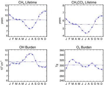
Fig. 3.Seasonal cycle of the globally averaged CH4and CH3CCl3
tropospheric lifetimes, OH abundance, and O3burden for the en-tire troposphere. Also shown are annual mean values of the above quantities (dashed-dotted lines).
Spivakovsky et al. (2000) and Prinn (2001) and well within the range of previously mentioned model studies.
A similar relation persisting between atmospheric methane lifetimes and hydroxyl radical concentrations, OH being the most important atmospheric CH4 sink, can be
used to further evaluate model performance in terms of photochemical activity. The annual mean tropospheric CH4
lifetime due to reaction with OH as calculated by the model amounts to 9.2 years. In the 2001 IPCC report (Prather et al., 2001) an estimate for this quantity has been given suggesting a an annual mean tropospheric methane lifetime of 9.6 years. LMDz-INCA is in quite close agreement with this IPCC assessment. Fig. 3 summarizes the seasonal cycle of the globally averaged chemical lifetimes of methane and methylchloroform, the hydroxyl radical abundance, and the tropospheric ozone burden. The model calculates global an-nual mean tropospheric values of 9.6×10⁵ molecules cm−3 and 303 Tg for the OH abundance and ozone burden, respectively.
Table 6.Break-down of annual average hydroxyl radical concentra-tions classified by tropospheric subdomains (105molecules cm−3). Horizontal domains: northern extratropics (NET, 90◦–30◦N), tropics (TRO, 30◦N–30◦S), southern extratropics (SET, 30◦– 90◦S); vertical domains: planetary boundary layer (PBL, below 750 hPa), free troposphere (FT, 750–500 hPa), upper troposphere and tropopause region (UT, 500–250 hPa), respectively. The rows and columns denoted byTOT andTOT, respectively, refer to the mean calculated over the specific horizontal layer or altitude range.
subdomain PBL FT UT TOT
NET 9.0 6.4 5.6 7.8
TRO 16.6 10.7 7.7 12.5
SET 5.3 4.4 4.5 5.4
TOT 11.9 8.1 6.4 9.6
From Table 6 it can be seen that the tropical planetary boundary layer has the highest oxidative capacity of all tro-pospheric subdomains with an annual mean OH abundance of 16.6×10⁵molecules cm−3. The oxidative capacity calcu-lated by the model decreases with increasing altitude, consis-tent with the current knowledge. Viewed over the entire alti-tude range, the tropical troposphere shows the highest oxida-tive capacity, in the southern extratropical troposphere OH concentrations are on average significantly lower.
Methane itself is a prognostic tracer in LMDz-INCA. The model takes into account various primary sources of CH4(cf.
Table 5), transport and mixing, tropospheric-stratospheric exchange, and atmospheric oxidation. A global sink of ap-proximately 30 Tg yr−1 due to consumption of CH4 by
methanotropic bacteria in soil has been identified (cf., e.g., Prather et al., 2001). The uncertainties around this processes are still quite high and are expressed in terms of an uncer-tainty factor of 2. This process, though, is not accounted for in our model at the present. The sink would account for approximately 5% of the global primary source of methane. Non-neglible but small on the global scale, this sink could potentially be of importance on the regional scale, since it is concentrated over the continental areas and varies with soil conditions.
The methane concentration at the surface as depicted in Fig. 4 exhibits a pronounced seasonal cycle in both the CMDL measurements and the model with a minimum dur-ing the local summer months when photochemical depletion via reaction with OH is most active. The observed magni-tude and phase of the seasonal variation in methane is fairly well reproduced by the model. Differences between model and observations are most pronounced at northern midlati-tude continental stations. The agreement between model and observations increases at stations in the tropics and the south-ern hemisphere representative of tropospheric background conditions. At these stations the model shows less diurnal variation which we contribute to a decreased influence of the
rapid photochemistry of NMVOC which also produces sig-nificant amounts of CH4. This absence of photochemistry on
short time-scales of hours or days could affect the compar-ison between climatological observations and the calculated methane concentration.
3.3 Nitrogen compounds
The importance of nitrogen compounds is a consequence of their role in the budget of other key tropospheric species, such as ozone and the hydroxyl radical. Odd nitrogen is mainly released in the form of NO, predominantly as a result of combustion processes (fossil fuel combustion, biomass burning) and soil microbial activity. Global lightning activity also represents a significant atmospheric source of NO. Once emitted, NO is rapidly converted by photochemical processes into other states of oxidation (NO2, NO3, N2O5) as well as
HNO3 and organic nitrates, including peroxyacetyl nitrate
(PAN).
A comparison of observed and calculated profiles of NOx
and PAN are shown in Figs. 5 and 6. The calculated NOx
mixing ratio is generally in good agreement with observa-tions, given the large spatial and time variability in this short-lived species. The typically ”C-shaped” profiles with higher mixing ratios in the PBL and the upper troposphere as well as decreased mixing ratios in the free troposphere are also well captured. The model, however, overestimates NOxover
Ireland during SONEX below 8 km which could be due to an overestimate of the anthropogenic NOxsource in EDGAR
v3.2 or the export of NOxfrom the continent being too strong
in our model over this region. The model underestimates NOx concentrations in the upper troposphere during
SUC-CESS.
Organic nitrates in general, and in particular peroxyacetyl nitrate (PAN), are chemically more stable compounds than NOx. PAN is the most abundant organic nitrate that has been
detected in the atmosphere resulting from a variety of organic precursors, such as isoprene, acetaldehyde, and alkanes (e.g. Roberts, 1990; Altshuller, 1993). Predominantly produced in the PBL by reaction of peroxyacetyl radicals with NO2, PAN
subsequently becomes subject to long-distance transport to remote environments and to the free troposphere, where it acts as a reservoir of NOx. Eventually, NOx is released
following thermal decomposition and photolysis (Crutzen, 1979; Kasibhatla, 1993; Moxim et al., 1996). PAN lifetimes vary from a few hours in the lower troposphere, where ther-mal decomposition effectively limits its residence time, to several months in the free and upper troposphere. LMDz-INCA also considers PAN analogs that derive from higher NMHC as well as other bulk organic nitrate species (cf. Ta-ble 1). They generally have shorter atmospheric lifetimes and, hence, significant concentrations are found only in the PBL.