Uncertainties of parameterized surface downward clear-sky shortwave and all-sky longwave radiation.

www.atmos-chem-phys.net/12/5077/2012/ doi:10.5194/acp-12-5077-2012

© Author(s) 2012. CC Attribution 3.0 License.

Chemistry

and Physics

Uncertainties of parameterized surface downward clear-sky

shortwave and all-sky longwave radiation.

S. Gubler, S. Gruber, and R. S. Purves

University of Zurich, Department of Geography, Zurich, Switzerland

Correspondence to:S. Gubler (stefanie.gubler@geo.uzh.ch)

Received: 17 September 2011 – Published in Atmos. Chem. Phys. Discuss.: 31 January 2012 Revised: 8 May 2012 – Accepted: 22 May 2012 – Published: 8 June 2012

Abstract.As many environmental models rely on simulating the energy balance at the Earth’s surface based on parameter-ized radiative fluxes, knowledge of the inherent model uncer-tainties is important. In this study we evaluate one parame-terization of clear-sky direct, diffuse and global shortwave downward radiation (SDR) and diverse parameterizations of clear-sky and all-sky longwave downward radiation (LDR). In a first step, SDR is estimated based on measured input variables and estimated atmospheric parameters for hourly time steps during the years 1996 to 2008. Model behaviour is validated using the high quality measurements of six Alpine Surface Radiation Budget (ASRB) stations in Switzerland covering different elevations, and measurements of the Swiss Alpine Climate Radiation Monitoring network (SACRaM) in Payerne. In a next step, twelve clear-sky LDR parameteri-zations are calibrated using the ASRB measurements. One of the best performing parameterizations is elected to esti-mate all-sky LDR, where cloud transmissivity is estiesti-mated using measured and modeled global SDR during daytime. In a last step, the performance of several interpolation meth-ods is evaluated to determine the cloud transmissivity in the night.

We show that clear-sky direct, diffuse and global SDR is adequately represented by the model when using measure-ments of the atmospheric parameters precipitable water and aerosol content at Payerne. If the atmospheric parameters are estimated and used as a fix value, the relative mean bias de-viance (MBD) and the relative root mean squared dede-viance (RMSD) of the clear-sky global SDR scatter between be-tween−2 and 5 %, and 7 and 13 % within the six locations. The small errors in clear-sky global SDR can be attributed to compensating effects of modeled direct and diffuse SDR since an overestimation of aerosol content in the atmosphere

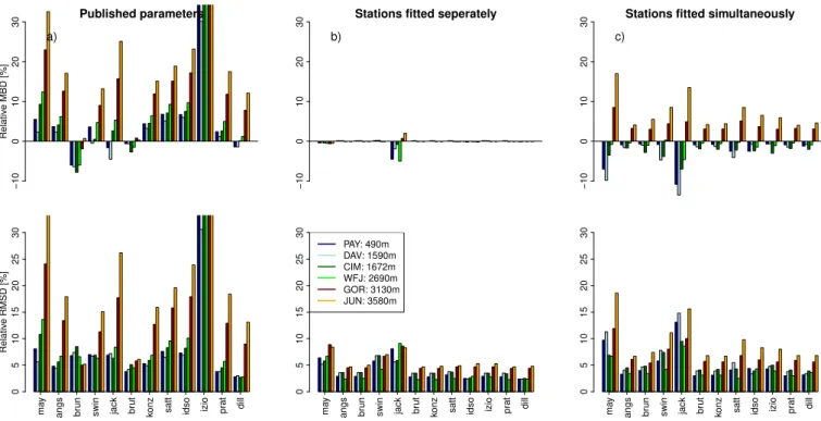
results in underestimating the direct, but overestimating the diffuse SDR. Calibration of LDR parameterizations to local conditions reduces MBD and RMSD strongly compared to using the published values of the parameters, resulting in rel-ative MBD and RMSD of less than 5 % respectively 10 % for the best parameterizations. The best results to estimate cloud transmissivity during nighttime were obtained by lin-early interpolating the average of the cloud transmissivity of the four hours of the preceeding afternoon and the following morning.

Model uncertainty can be caused by different errors such as code implementation, errors in input data and in estimated parameters, etc. The influence of the latter (errors in input data and model parameter uncertainty) on model outputs is determined using Monte Carlo. Model uncertainty is pro-vided as the relative standard deviationσ_relof the simulated frequency distributions of the model outputs. An optimistic estimate of the relative uncertaintyσ_rel resulted in 10 % for the clear-sky direct, 30 % for diffuse, 3 % for global SDR, and 3 % for the fitted all-sky LDR.

1 Introduction

the knowledge about the complex interactions between the atmosphere, the Earth surface and subsurface. In mountain areas, changes in the energy budget can already be observed at small distances due to the strong topographic variability.

Modeling energy fluxes and their uncertainties at the land surface is a key step in many model applications. A wide variety of models estimating SDR or LDR have been pro-posed in the literature, ranging from complex physical mod-els using radiative transfer schemes and integrating aerosol and gaseous profiles of the atmosphere (e.g. LOWTRAN or MODTRAN) to empirical models based on relations be-tween meteorological variables. For many applications, so-phisticated models such as MODTRAN are inappropriate due to their complexity, required input data and computa-tional effort. This study is based on the clear-sky broad-band radiation model by Iqbal (1983, based on Bird and Hulstrom, 1980, 1981) and empirical parameterizations for clear- and all-sky LDR found in the literature (e.g. Brutsaert, 1975; Konzelmann et al., 1994; Pirazzini et al., 2000). The performance of many of these parameterizations has exten-sively been evaluated (e.g. Gueymard, 1993, 2003a,b, 2011; Crawford and Duchon, 1998; Battles et al., 2000; Pirazzini et al., 2000; Nimiel¨a et al., 2001a,b), but sensitivity or uncer-tainty studies are rare in the literature (e.g. Gueymard, 2003b; Schillings, 2004; Badescu et al., 2012). Thus we focus on evaluating the Iqbal (1983) clear-sky SDR model and fitting the LDR parameterization to six locations at different eleva-tions in Switzerland, and estimating model sensitivities and uncertainties due to different error sources.

The Iqbal (1983) model has been chosen since it has shown to reproduce SDR reasonably well under different cli-matic settings (Gueymard, 1993; Battles et al., 2000; Guey-mard, 2003b). Furthermore, it has been frequently used in impact model applications (e.g. Corripio, 2002; Gruber, 2005; Machguth et al., 2008; Helbig et al., 2009) as well as other studies aiming at an optimal use of solar power, for example (Schillings, 2004). The Iqbal (1983) model as-sumes a homogeneous atmosphere and uses an isotropic view factor approach. Due to these simplifications, input is lim-ited to a few quantities such as screen-level temperature (i.e. the temperature at the height of the measurement device, here 2 m above the ground), relative humidity and atmo-spheric pressure, and model parameters consist of the amount of ozone, aerosols and water vapor in the overlying atmo-sphere, among others, to determine the transmission respec-tively scattering of the solar rays. Under clear skies and non-polluted conditions, transmittance from ozone, precipitable water, aerosols, mixed gases and the Rayleigh transmittance cause most atmospheric attenuation (Gueymard, 2003a). In the past, these parameters could “not be easily determined from normally available information” (Dozier, 1980). Nowa-days, ozone, aerosol content and water vapor is measured and can be obtained from Aeronet or satellite data such as MODIS for many locations, the datasets however often have spatial or temporal gaps (Gueymard, 2003a). Using this data

therefore requires temporal interpolation and spatial extrap-olation causing errors that are propagated into model outputs (Gueymard, 2003b). Practical model applications incorporat-ing parameterizations of the downward radiation as a drivincorporat-ing factor of other environmental processes are usually restricted to few input quantities such as the variables recorded at or-dinary weather stations. Such impact models often treat pa-rameters such as ozone, aerosol content and water vapor as constants (Longman et al., 2012). On one hand, this approach reduces the time and data management effort of a model user, on the other hand it introduces a considerable source of un-certainty and error into the model (Gueymard, 2003b; Bade-scu et al., 2012).

This study investigates the uncertainty of the Iqbal (1983) model due to uncertainties in inputs and the above men-tioned simplifications concerning the estimated atmospheric parameters. A Monte Carlo based uncertainty analysis is per-formed based on previously determined input error and pa-rameter probability distributions. The latter are determined using high quality measurements and/or established param-eterizations of the correspondent parameter, while the input measurements are obtained from MeteoSwiss. In a next step, some of the most commonly used clear-sky LDR parameter-izations are fitted to local conditions in Switzerland, result-ing in the identification of the most appropriate parameteri-zations. For one of these parameterizations, the total output uncertainty is assessed based on input and parameter uncer-tainty similarly as discussed above. Clouds are one of the main LDR forcings. Since cloud cover is only rarely mea-sured and measurements are error-prone, it is common to es-timate the cloud transmissivity as the ratio of the measured and modeled clear-sky global SDR during daytime. During the night, when this approach is not feasible, cloud trans-missivity is interpolated. In a last step, we therefore examine different cloud transmissivity interpolations, and propagate inherent uncertainties into all-sky LDR model outputs.

Thus, the aims of the present study are:

– to evaluate the clear-sky SDR model by Iqbal (1983) at six sites in Switzerland;

– to calibrate diverse clear- and all-sky LDR models and to assess the best all-sky parameterizations for impact modeling studies in Switzerland;

– to study the output of different interpolation techniques of the cloud transmissivity during nighttime; and – to estimate the total output uncertainty of the clear-sky

SDR model by Iqbal (1983) and one of the all-sky LDR models due to uncertainties in input variables and pa-rameters.

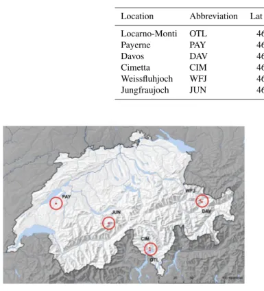
Table 1.Meta data of the MeteoSwiss stations. At each place, one ANETZ and one ASRB station is located.

Location Abbreviation Lat (deg N) Long (deg E) Ele [m]

Locarno-Monti OTL 46.1726 8.7874 367

Payerne PAY 46.8116 6.9424 490

Davos DAV 46.8130 9.8435 1590

Cimetta CIM 46.2010 8.7908 1672

Weissfluhjoch WFJ 46.8333 9.8064 2690

Jungfraujoch JUN 46.5474 7.9853 3580

Fig. 1.Locations of the six MeteoSwiss stations in Switzerland (geodata © swisstopo). The coordinates of the locations are from MeteoSwiss (http://www.meteoswiss.admin.ch).

the sensitivity and the uncertainties in the clear-sky SDR and LDR model, and the validation and calibration methods are introduced. Then, the results are presented and discussed.

2 Data description

This modeling study is performed for six locations in Switzerland (Fig. 1, Table 1). The model is run with mea-surements from MeteoSwiss (Sect. 2.1) and estimated pa-rameters (Sect. 2.2). The uncertainties in the input data and the parameters were assigned based on expert knowledge and literature, or were estimated based on representative mea-surements. Perceptual and structural model errors (cf., Beck, 1987; Beven, 1993; Kavetski et al., 2003; Gupta et al., 2005) are not investigated.

The data are structured as (a) input data, (b) physical and empirical model parameters and (c) validation data.

2.1 Input and validation data

The input data is obtained from the MeteoSwiss automatic meteorological network (ANETZ). The Alpine Surface Ra-diation Budget (ASRB, Philipona et al., 1996) network data serves for validation (SDR) and calibration (clear-sky and all-sky LDR). The number of study sites is restricted to the

intersection of both networks. The study is performed with hourly data ranging from 1996 to 2008, resulting in 113 976 data points. Since synoptic cloud observations are rare (they exist only for 3 stations of this study) and error-prone, clear-sky hours are estimated according to the clear-clear-sky index (CSI) introduced by Marty and Philipona (2000). The num-ber of clear-sky hours varies between 25 000 and 38 000. The measurement errors are assumed to be normally distributed with zero mean. Standard deviations of the input and valida-tion data (Table 2) were obtained from MeteoSwiss (courtesy of Rolf Philipona Philipona et al., 1995). All the measured data are denoted in equations with a superscript ∗(for exam-ple,T∗denotes measured air temperature).

2.2 Physical and empirical model parameters 2.2.1 SDR

The main focus of this study concerning modeled SDR lies on the estimation of the total output uncertainty of the Iqbal (1983) model due to the absorption, scattering and trans-mittance of the incoming solar radiation in the atmosphere, plus their reflection at the ground surface. Uncertainties in ozone column data, aerosol, precipitable water and in ground albedo are investigated and the probability density functions of each parameter are determined. Mean and standard devia-tion of the parameters are estimated using high quality mea-surements recorded in Switzerland, or using established pa-rameterizations found in the literature. All uncertainty ranges are compared to estimates by Gueymard (2003b), and result to be representative. The uncertainty in Rayleigh and mixed gas transmittance is not investigated since it has limited in-fluence on modeled SDR (Gueymard, 2003b).

Aerosol:Attenuation effects of scattering and absorption by aerosols were modeled according to ˚Angstr¨om (1929, 1930):

ταλ=β(λ/λ0)−α, (1)

whereα is the wavelength exponent (also called ˚Angstr¨om exponent), β is the turbidity coefficient and λ0=1000 nm

Table 2.Input, model parameters and validation data with uncertainty distributions, meanµand standard deviationσ. Note that the dis-tribution for the ANETZ and ASRB measurements concern the error of the measurement (denoted with E), whereas the disdis-tribution in the parameters concerns the parameter value itself. Since ground albedo varies temporally and spatially, its distribution is estimated for each station and each month separately (Table B1).

Measurement Distribution µ σ Unit Symbol

Input Air temperature Normal (E) 0 0.2 K T∗

Relative humidity Normal (E) 0 5 % h∗_r

Air pressure Normal (E) 0 0.2 hPa p∗

Parameter Ozone column Lognormal 314 38 DU l

˚

Angstr¨om exponent Normal 1.38 0.46 α

˚

Angstr¨om turbidity Lognormal 0.039 0.05 β

PrecWatConstant Lognormal 47 0.38 g K cm−2hPa−1 aw

Ground Albedo Lognormal ρ_g

Cloud transmissivity Normal (E) 0 0.08 τc

Validation Global SDR Normal (E) 0 2 % W m−2 SDR∗_glob

LDR Normal (E) 0 2 % W m−2 LDR∗_in

turbidity coefficientβ are determined from a linearised ver-sion of the ˚Angstr¨om’s law in Eq. (1) (Gueymard, 2011):

lnταλ=lnβ−αln(λ/λ0). (2)

To estimateαandβ, we usedταλ for wavelengths between 380 and 1020 nm. According to the resultant frequency dis-tributions,αis assumed to be normally distributed with lower limit zero, andβ is represented by a trimmed log-normal distribution with an upper limit equal to 0.5. The estimated mean value forαof 1.38 is close to the recommended value by ˚Angstr¨om (1930)α₌1.3.

Water vapor:The effect of absorption due to water va-por contained in the atmosphere is estimated using the pre-cipitable waterw (Eq. A10). The precipitable water is the water contained in a column of unit cross section extending from the Earth’s surface to the top of the atmosphere. Data of precipitable water is rarely available (Iqbal, 1983), and is thus often parameterized. Historical overviews of precip-itable water parameterizations are given in Iqbal (1983) and Okulov et al. (2002). Here, the parameterization found in Re-itan (1963); Leckner (1978) and Prata (1996) is used:

w₌aw

h∗_rp_s

T∗ , (3)

wherea_wis estimated (Eq. 4),h∗_r is the measured relative hu-midity in fractions of one,p_sis saturated water vapor pres-sure in hPa and T∗ is screen-level temperature in K. The vapor pressure in saturated air is determined as a function of air temperature (Flatau et al., 1992). The parameter aw

[10g K hPa−1cm−2] is estimated as (Prata, 1996):

aw=

M_w

R·k·ψ, (4)

whereMw=18.02 g mol−1is the molecular weight of water

vapor,R₌8.314 J K−1_mol−1 _{is the universal gas constant}

and ψ=1.006 is a constant. Further, k=kw+Tγ∗, where kw=0.44 km−1is the inverse water vapor scale height

(Re-itan, 1963; Brutsaert, 1975) andγ is the lapse rate. The un-certainty ofa_w is estimated by propagating the uncertainty inherent in the air temperature measurements and the lapse rate. The lapse rate is assumed to be normally distributed with mean equal to the standard value of−6.5 K km−1 for the Alps and standard deviation of 1 K km−1, based on the vestigations of Hebeler and Purves (2008). Following the in-vestigations of Foster et al. (2006),awandware assumed to

be lognormally distributed. The uncertainty inawis around

1 %. By propagating the input measurement errors through Eq. 3, we observe an estimated uncertainty in precipitable water greater than 100 % (see Fig. 5), which is in accordance with Gueymard (2003b).

Ozone: MeteoSwiss provides accurate ozone column measurements in Arosa (Staehelin et al., 1998) on about two thirds of all days during the year. Ozone is assumed to be lognormally distributed. The estimated standard deviation of the ozone frequency distribution is around 12 % of the mean ozone, implying that the assumed uncertainty represents the ozone measurement uncertainty (5 to 30 %) as estimated by Gueymard (2003b) well.

Table 3.Parameterizations of clear-sky emissivity.pvis the water vapor pressure [hPa], andT∗the measured temperature [K].x1, x2and

x₃denote the empirical parameters.

Publication Abbr. Eq. ǫcl x1 x2 x3

Maykut and Church (1973) may 18 x1 0.7855

˚

Angstr¨om (1915) angs 8 x1−x2·10−x3·pv 0.83 0.18 0.067

Brunt (1932) brun 7 x1+x2·√pv 0.52 0.065

Swinbank (1963) swin 9 x1·T∗2 9.365×10−6

Idso and Jackson (1969) jack 10 1−x1·exp(−x2·(273−T∗)2) 0.261 7.77×10−4

Brutsaert (1975) brut 12 x1·(pvT∗)1/x2 1.24 7

Konzelmann et al. (1994) konz 13 0.23₊x1·(100T∗pv)1/x2 0.484 8

Satterlund (1979) satt 14 x1·(1−exp(−p

T∗ 2016

v )) 1.08

Idso (1981) idso 11 x1+x2·pv·exp(_Tx3∗) 0.7 5.95×10−5 1500

Iziomon et al. (2003) izio 16 1₋x1·exp(−x2·Tpv∗) 0.43 11.5

Prata (1996) prat 15 1−(1+46.5·_Tpv∗)·exp(−(x1+x2·46.5·_Tpv∗)x3) 1.2 3 0.5

Dilley and O’Brien (1997) dill 17 (x1+x2·(273T∗.16)6+x3·(

46.5pv

T∗

2.5 )0.5)/(σSBT∗4) 59.38 113.7 96.96

2.2.2 LDR

The LDR parameterizations contain empirical parameters (Table 3) which originally were fitted to measurements at specific research sites (see Sect. 3.1.2 for details). In this study, we fit the selected parameterizations to the measure-ments at the six study sites in Switzerland, and identify reli-able parameter values for the local conditions. The confind-ence intervals of the non-linear least-quares parameter esti-mation are used to quantify the uncertainty of the parame-ters. Clouds are a major forcing of LDR, and are estimated using measured and modeled global SDR. Uncertainties in modeled SDR thus are propagated to cloud transmissivity through Eq. (19). The standard deviation results in approx-imately 0.08 for modeled cloud transmissivity.

3 Methods

3.1 Model formulations

In this section, we give a brief overview of the model formu-lations and parameterizations used in the study.

3.1.1 Clear-sky SDR

In a first step, the clear-sky broadband global SDR is esti-mated (Iqbal, 1983, model C). For details the reader is asked to refer to Appendix A. The model estimates the direct SDR by calculating the radiation at the top of the atmosphere (Cor-ripio, 2002), and the attenuation of the solar radiation by ozone, water vapor, aerosol and dry-air particles in the at-mosphere. Then, the diffuse SDR due to Rayleigh-scattering, scattering by aerosols and the multiple reflection of the sun

rays between the Earth’s surface and the atmosphere is es-timated. Direct and diffuse radiation sum up to the global SDR. Radiation due to scattering from surrounding terrain is included. However, it only accounts for a very small part of the total global SDR since the study locations are situated in locally flat terrain.

3.1.2 Clear-sky LDR

Clear-sky LDR is determined by the Stefan-Boltzmann law:

LDRcl=ǫatm·σSB·Tatm4 , (5)

where σ_SB=5.67×10−8W m−2K−4 denotes the Stefan-Boltzmann constant, ǫ_atm the bulk emissivity andT_atm the effective temperature of the overlying atmosphere. In prac-tice, LDRclis estimated as:

LDRcl=ǫcl(pv, T∗)·σSB·T∗4, (6)

whereT∗denotes absolute air temperature (K) at the refer-ence height of 2 m above the ground andǫcl is the

parame-terized clear-sky emissivity. In the present study, twelve pa-rameterizations (Table 3) are calibrated with measurements in Switzerland, and the most suitable ones are determined. The parameterizations are shortly presented in the following paragraph.

Estimating clear-sky emissivity based on water vapor pres-sure and temperature meapres-surements has a long history. Brunt (1932) for example observed a linear relationship between

ǫ_cland√p_v. He showed that fitting a linear regression line:

represented clear-sky emissivity better than the ˚Angstr¨om (1915) formula:

ǫ_cl=x₁₊x_2×10−x3pv (8)

for measurements made in Uppsala (Askl¨of, 1920). The parameter values for Brunt (1932) however vary signifi-cantly for different locations due to different rates of changes of air temperature and vapor pressure with elevation, but also due to differing methods estimating vapor pressure (Brunt, 1932). The parameters used here were estimated with monthly measurements from Benson, UK (Dines, 1921). Swinbank (1963) states that the relationship betweenǫcland

pv found by ˚Angstr¨om (1915) and Brunt (1932) basically

arise from the relationship between humidity and tempera-ture, and would only be appropriate for an atmosphere of constant grayness (e.g. Idso and Jackson, 1969). A better representation of LDRclwas found using temperature alone

(Swinbank, 1963):

LDRcl=x1σSBT∗6, (9)

withx1=5.31×10−13 in Australia,x1=5.21×10−13 for

the Benson measurements, and LDRclin mWcm−2. Idso and

Jackson (1969) proposed the relation:

ǫcl=1−x1exp(−x2(273−T∗)2), (10)

assuming that just above 273 K clear-sky emissivity may be described as an exponential function of temperature, and that the variation in ǫcl is symmetrical around the

freez-ing point. They proved their relationship with x1=0.261

andx₂₌7.77×10−4to provide more reliable results than ˚

Angstr¨om (1915); Brunt (1932) and Swinbank (1963), and tested the parameterization for measurements in Alaska, Ari-zona, Australia and the Indian Ocean. Some years later, Idso (1981) established a physically based formula using new measurements of the total LDR for all wavelengths and the portions contained within the 10.5- to 12.5 µm and the 8 to 14 µm bands, resulting in:

ǫcl=x1+x2pvexp(x3/T∗) (11)

x₁₌0.7, x₂₌5.95×10−5, x₃₌1500.

This is one of the first attempts to express the clear-sky effec-tive emissivity in dependence of both temperature and water vapor. Earlier, Brutsaert (1975) suggested:

ǫ_cl=x₁(pv T∗)

1/x2_{, x}

1=1.24, x2=7 (12)

by integrating the Schwarzschild’s radiative-transfer equa-tion for simple atmospheric profiles. The formula can be re-duced toǫcl=0.553pv1/7forT =288 K since it not very

sen-sitive to changes in temperature (Brutsaert, 1975). To include the effect of greenhouse gases other than vapor pressure on

LDR, Konzelmann et al. (1994) changed Brutsaert (1975) equation to:

ǫcl=0.23+x1(

p_v

T∗)

1/x2_{, (13)}

where x1=0.443 and x2=8 were optimal for

measure-ments on the Greenland ice sheet. Note thatpvis in Pascal in

the Konzelmann et al. (1994) publication. To be consistent, we useǫcl=0.23+x1(100_T∗pv)1/x2 here. Another physically

based equation taking into account both temperature and wa-ter vapor was proposed by Satwa-terlund (1979) to ensure that ideal black body radiation is not exceeded by any extreme temperature or humidity value. Tested with measurements from Aase and Idso (1978) at Sidney, Montana, his formula resulted in:

ǫcl=x1·(1−exp(−p

T∗ 2016

v )),wherex1=1.08. (14)

Prata (1996) found:

ǫ_cl=1−(1+u)exp(₋(x₁₊x₂u)x3), (15) withu₌46.5_Tpv_∗ to represent the full long-wave spectrum such thatǫ_cl→1−exp(₋xx3

1 )=const foru→0 andǫcl→

1 foru_{→ ∞}. Prata (1996) estimated x₁₌1.2, x₂₌3 and

x₃₌0.5 for the measurements of Robinson (1947, 1950), the data that was also used by Brutsaert (1975). Iziomon et al. (2003) suggested another equation:

ǫcl=1−x1exp(−x2

p_v

T∗), x1=0.43 andx2=11.5 (16)

which was fitted to measurements performed in Germany, whereas Dilley and O’Brien (1997) estimated LDRcl=(1−

exp(₋1.66τ ))σ_SB·T∗whereτ ₌2.232−1.875(T /273.16)₊

0.7356(w/2.5)1/2is the grey-body optical thickness. His aim was to represent the main emission processes of the lower at-mosphere, i.e. emission from water vapor and CO2.

Approxi-mating the exponential by power series and neglecting all but the lowest order multinomials leads to:

LDRcl=x1+x2(T∗/273.16)6+x.3 p

w/2.5, (17)

x1=59.38, x2=113.7, x3=96.96.

The exponent of temperature is in accordance with the find-ings by Swinbank (1963). The simples equation assuming constant emissivity:

ǫcl=const (18)

resulted convenient for Maykut and Church (1973) in Point Barrow, Alaska, and K¨onig-Langlo and Augstein (1994) for Arctic and Antarctic measurements.

3.1.3 Cloud transmissivity and cloud cover

transmissivityτ_cas the ratio of the estimated clear-sky global SDRgloband the measured global SDR∗_glob(e.g. Greuell et al.,

1997):

τc=

SDR∗_glob SDRglob

. (19)

Note that τc<1 if the sky is overcast, and τc=1

de-notes clear-sky conditions. Most parameterizations for all-sky LDR are based on the cloud-factorN, which is zero if the sky is completely clear, and one if the sky is cloud-covered. The linear relation betweenτ_candN(Crawford and Duchon, 1998):

N₌1−τ_c (20)

is used in this study. Different relationships involving a quadratic dependence ofN andτc (Greuell et al., 1997) or

even containing further parameters such as the relative hu-midity (Sicart et al., 2006) can be found in the literature. 3.1.4 All-sky LDR

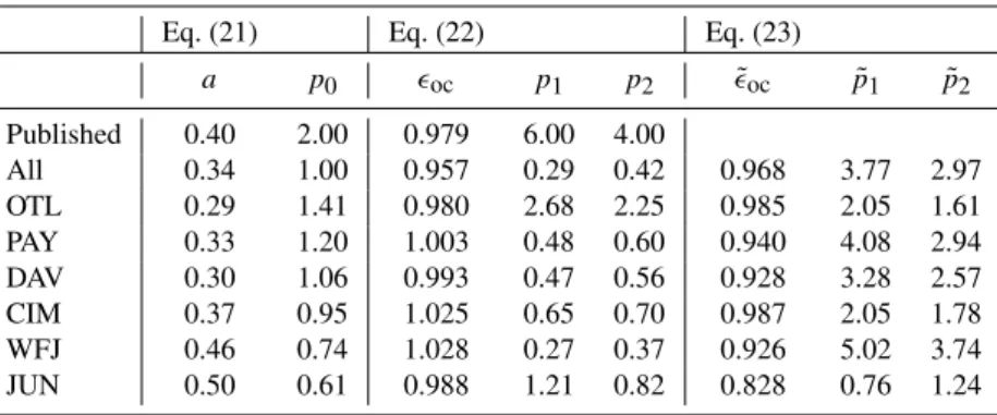
Existing all-sky LDR parameterizations were summarized and tested for measurements recorded at Ny- ˚Alesund, Spits-bergen by Pirazzini et al. (2000) and result in the following two equations:

LDRall=LDRcl·(1+aNp0) (21)

and

LDRall=(ǫcl(1−Np1)+ǫocNp2)σSBT∗4, (22)

whereǫclis the estimated clear-sky emissivity,a, p0, p1and

p2 are parameters and ǫoc is the cloud emissivity. In this

study, a slightly modified formula is further examined: LDRall=(ǫclτcp1˜ + ˜ǫoc(1−τcp˜2))σSBT∗4, (23)

where the all-sky LDR is determined based on cloud trans-missivity directly. This has the advantage of not having to choose a conversion fromτctoN, but the disadvantage that

a comparison with published values for the parametersp_˜1,p˜2

andǫ˜ocis not possible.

3.1.5 Interpolation of cloud transmissivity during nighttime

The cloud transmissivity can, during daytime, be estimated according to Eq. 19. During the night, it is often determined by linearly interpolating between the last point in time at sun-set, and the first point in time in the morning, or using a con-stant interpolation taking a mean cloud amount value from the preceding afternoon (Lhomme et al., 2007). These in-terpolated cloud transmissivity estimates are rarely validated due to the lack of available data. Here, we use different in-terpolation techniques, calculate the all-sky LDR during the night and evaluate the outputs with the ASRB measurements. The interpolation methods are:

1. linear interpolation between a mean value ofx points in time (where each point in time represents an hourly value) before sunset andxpoints in time after sunrise, 2. constant interpolation of the mean value ofx points in

time before sunset,

3. constant interpolation of the mean value ofx points in time after sunrise,

wherex₌1,2, ...,6. 3.2 Model evaluation

The models are evaluated by a) investigating the model sensi-tivities to certain previously selected parameters, b) assessing the models’ output uncertainty coming from uncertainty in input data and model parameters, c) comparing model out-puts to measurements for validation, and d) calibrating di-verse empirical and physical LDR parameterizations to con-ditions in Switzerland. To investigate a) and b), a probabil-ity densprobabil-ity function (often called prior distribution, Table 2) is assigned to estimate the errors in the input variables and the parameters (Sect. 2.2). The errors in the parameters and input measurements are assumed to be independent. These distributions form the basis to analyze the local sensitivity of the model to each parameter (Sect. 3.2.1), and to perform a Monte Carlo based uncertainty analysis (Sect. 3.2.2). Us-ing the mean parameter values and zero error for the input measurements, a simulation is run and the models are val-idated (Sect. 3.2.3). Calibration of the LDR parameteriza-tions is performed based on non-linear least-squares estima-tion (Sect. 3.2.4).

3.2.1 Sensitivity analysis

SDR:Local relative sensitivities of direct, diffuse and global clear-sky SDR to ozone, precipitable water, the ˚Angstr¨om pa-rameters and ground albedo are estimated. The sensitivities are estimated for constant path lengthmr=2, the path length

estimated for a mean solar zenith angle of around 60 degrees at Jungfraujoch. Each model parameterθi is varied, unless the interval exceeds the physically possible values, within the interval[µi−2σi, µi+2σi]while all other parameterθj6=iare kept fixed atµj. Thereby, the influence of 97 % of the most plausible parameter values on SDR is investigated.

0 5000 10000 15000 20000

0

10

20

30

40

50

Cimetta: 9th June 1996

Simulation Number

Standard de

viation [W/

m

2]

Direct SDR Diffuse SDR Global SDR

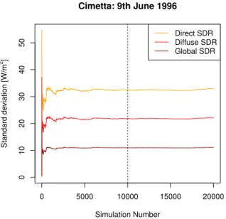
Fig. 2.Standard deviations of the model simulations at Cimetta. 10 000 model simulations result sufficient to reach stable standard deviations of the output frequency distribution.

3.2.2 Uncertainty assessment

Monte-Carlo based methods are widely used to derive the frequency density of the output of a model due to the sim-ple imsim-plementation even for comsim-plex, non-linear models. 10 000 model simulations were sufficient to estimate total model output uncertainty (Fig. 2). The standard uncertainty of the model is defined as the standard deviationσt,absof the

model result at each time step (JCGM, 2008). The relative uncertainties are σt,rel:=σt,abs/µt. The 90 %-quantile and the median of the relative uncertainties for all time steps are estimated, and used as conservative respectively confidence estimates of the total output uncertainty. Further, a function

f (SDR)₌σ_{SDR, rel}is fitted to the relative uncertainties

us-ing non-linear least-squares regression to derive the relative uncertainty in dependence of the modeled radiation. 3.2.3 Validation

Clear-sky global SDR and all-sky LDR are validated using the ASRB measurements (Sect. 2.1). The models are eval-uated for a simulation which is performed with the mea-sured input time series (assumed error-free) and the fixed pa-rameter valuesµ(Table 2). According to Gueymard (2011), model performance is measured using the mean bias de-viance (MBD) and the mean root squared dede-viance (RMSD) expressed in percent of the mean measured radiation. This naming is preferred over the often found mean bias error (ME) and root mean squared error (RMSE) to emphasize that a deviation between the model output and the measured value can come from both model error and measurement un-certainty (Gueymard, 2011). The MBD is a simple and very

familiar measure that neglects the magnitude of the errors (i.e. positive errors can compensate for negative ones):

MBD= 1

y∗· Pn

t=1et

n (24)

MBD_∈(_−∞,_∞),MBDperf=0,

whereet:=yt−yt∗ are the residuals of the models. Here, yt denotes the modeled output variable, andyt∗is the corre-sponding measured variable. The RMSD is:

RMSD= 1

y∗· v u u t

1

n n

X

t=1

e2_t, (25)

RMSD_{∈ [}0,_∞),RMSDperf=0.

It accounts for the average magnitude of the errors and puts weight on larger errors, but does not account for the direction of the errors. For clarity, both MBD and RMSD are expressed in percents throughout the manuscript. The correlation coef-ficient R measures the linear agreement between the modeled and the measured variable:

R=

Pn

t=1(yt−y)(yt∗−y∗)

q Pn

t=1(yt−y)2(yt∗−y∗)2

(26)

R∈ [−1,1],Rperf=1,

The coefficient of determination R2indicates the amount of variation in one variable explained through the other. 3.2.4 LDR calibration using non-linear least-squares Non-linear least-squares estimation (Bates and Watts, 1988; Bates and Chambers, 1992) is used to fit the clear-sky LDR parameterizations to observational data. In a first step, the clear-sky emissivity is estimated as:

ǫcl=

LDR∗ in,cl

σ_SBT∗4, (27)

where both LDR∗

in,clandT∗are measurements of the ASRB

stations. Then, the parameterizations presented in Table 3 are fitted to ǫcl. The start values for the non-linear estimation

are the parameters presented in the respective publications. Thereby, optimal parameter values are obtained for each sta-tion. Furthermore, the parameterizations are fitted simulta-neously to all stations, resulting in one single set of optimal parameters. Clear-sky situations are determined according to Marty and Philipona (2000); D¨urr and Philipona (2004).

4 Results

4.1 Clear-sky SDR 4.1.1 Validation

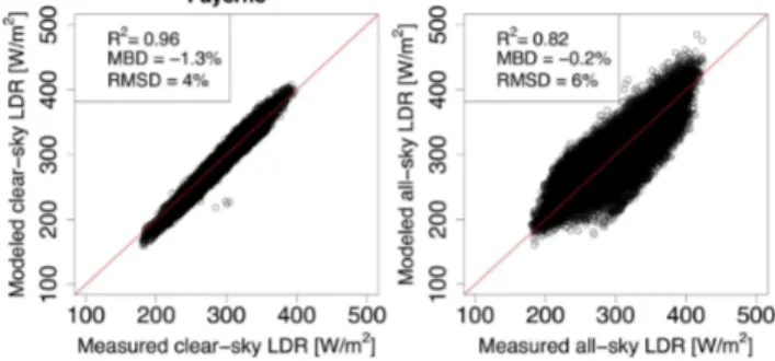
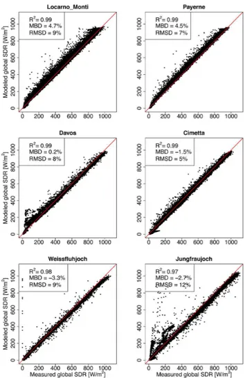
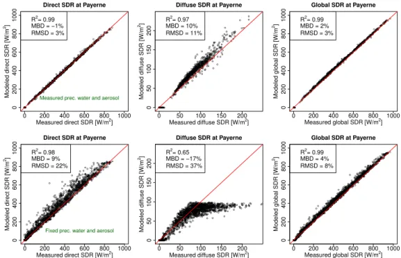
Modeled clear-sky global SDR is validated using the ASRB measurements. In general, a good linear agreement between model output and the measurements is observed (Fig. 3). The larger relative errors for low radiation can be attributed to the larger path length and thus higher influence of the es-timated parameters ozone, precipitable water, aerosol con-tent and ground albedo. Further, errors in cloud cover esti-mation by Marty and Philipona (2000); D¨urr and Philipona (2004) might be responsible for some of the scatter observed at Jungfraujoch, for example (Fig. 3). To confirm the va-lidity of the Iqbal-model for conditions in Switzerland, a model experiment was additionally performed using mea-surements of the atmospheric parameters (precipitable water,

˚

Angstr¨om parameterα andβ), and measured diffuse SDR in Payerne from the Swiss Alpine Climate Radiation Moni-toring network (SACRaM) of MeteoSwiss. We see that the Iqbal (1983) model performs satisfactorily when using mea-sured atmospheric parameters (Fig. 4, top). The scatter in dif-fuse SDR is normal for simple models such as the one by Iqbal (1983) (personal communication with C. Gueymard). Assuming that measurements of the atmospheric parameters do not exist, the diffuse SDR indicates large errors of−17 % (MBD) and 37 % (RMSD) compared to 10 % (MBD) and 11 % (RMSD) when using the measurements (Fig. 4). Fur-ther, a limiting value of around 100 W m−2in modeled dif-fuse SDR arises from an underestimation of the aerosol tent. Global SDR however is modeled satisfyingly using con-stant values of the atmospheric parameters since the diffuse SDR only accounts for around one tenth of global SDR, and since errors due to “incorrect” aerosol content in direct and diffuse SDR are of opposite sign and compensate for each other (see Sect. 4.1.2).

To check for systematic errors, the residualset were cor-related with the input variables and the sun elevation. While for the input variables the correlations are low (₋0.2<R<

0.2), errors slightly correlate with sun elevation (between 0 and 0.4 for direct, around−0.4 for diffuse and between−0.3 and 0.2 for global SDR). For direct SDR, the residuals scat-ter more (towards positive values) above the freezing point and for a relative humidity of around 60 %, similarly the dif-fuse SDR (but in opposite direction). Due to compensating effects, this is not observed for global SDR. Since the corre-lations are not large, systematic errors are not further inves-tigated.

One restriction already mentioned above must be kept in mind: clear-sky hours are based on the cloud estimation of Marty and Philipona (2000); D¨urr and Philipona (2004) and thus error-prone. This might be a cause for some of the scat-ter in Fig. 3 at Jungfraujoch, for example. To analyze the

ef-Fig. 3.Scatter plots of global modeled and measured SDR at all locations. The solid red line indicates the perfect fit.

fect of the clear-sky estimation, the validation measures were further estimated for clear-sky hours using synoptic cloud observations at the three stations Jungfraujoch, Payerne and Locarno-Monti. Since the overall picture of the model eval-uation did not change the analysis strongly, the results of the clear-sky evaluation presented here are assumed to be reli-able. A further indication of the validity of the approach is that the errors in the modeled clear-sky radiation do not cor-relate with the D¨urr and Philipona (2004) cloud cover esti-mates.

4.1.2 Sensitivity of the clear-sky SDR