www.geosci-model-dev.net/8/697/2015/ doi:10.5194/gmd-8-697-2015
© Author(s) 2015. CC Attribution 3.0 License.
Mechanistic site-based emulation of a global ocean biogeochemical
model (MEDUSA 1.0) for parametric analysis and calibration: an
application of the Marine Model Optimization Testbed
(MarMOT 1.1)
J. C. P. Hemmings1,2, P. G. Challenor3,1, and A. Yool1
1National Oceanography Centre, Southampton, SO14 3ZH, UK 2Wessex Environmental Associates, Salisbury, UK
3College of Engineering, Mathematics and Physical Sciences, University of Exeter, Exeter, EX4 4QF, UK
Correspondence to:J. C. P. Hemmings ([email protected])
Received: 7 July 2014 – Published in Geosci. Model Dev. Discuss.: 25 September 2014 Revised: 27 January 2015 – Accepted: 16 February 2015 – Published: 23 March 2015
Abstract.Biogeochemical ocean circulation models used to investigate the role of plankton ecosystems in global change rely on adjustable parameters to capture the dominant bio-geochemical dynamics of a complex biological system. In principle, optimal parameter values can be estimated by fit-ting models to observational data, including satellite ocean colour products such as chlorophyll that achieve good spa-tial and temporal coverage of the surface ocean. However, comprehensive parametric analyses require large ensemble experiments that are computationally infeasible with global 3-D simulations. Site-based simulations provide an efficient alternative but can only be used to make reliable inferences about global model performance if robust quantitative de-scriptions of their relationships with the corresponding 3-D simulations can be established.
The feasibility of establishing such a relationship is in-vestigated for an intermediate complexity biogeochemistry model (MEDUSA) coupled with a widely used global ocean model (NEMO). A site-based mechanistic emulator is con-structed for surface chlorophyll output from this target model as a function of model parameters. The emulator comprises an array of 1-D simulators and a statistical quantification of the uncertainty in their predictions. The unknown parameter-dependent biogeochemical environment, in terms of initial tracer concentrations and lateral flux information required by the simulators, is a significant source of uncertainty. It is approximated by a mean environment derived from a small ensemble of 3-D simulations representing variability of the
target model behaviour over the parameter space of interest. The performance of two alternative uncertainty quantifica-tion schemes is examined: a direct method based on compar-isons between simulator output and a sample of known target model “truths” and an indirect method that is only partially reliant on knowledge of the target model output.
1 Introduction
A need for better understanding of the role marine biota will play in influencing the nature and rate of global change in re-sponse to human activities has led to the inclusion of process-based models of ocean biogeochemistry in ocean circula-tion models (Sarmiento et al., 1993) and more recently in models of the whole Earth system (Séférian et al., 2013). They are designed to capture the dominant responses of com-plex ecosystems to variability in the physical environment. The biogeochemistry models vary in complexity from simple models in which the biota are represented by single phyto-plankton and zoophyto-plankton types (e.g. Six and Maier-Reimer, 1996; Palmer and Totterdell, 2001) to more complex func-tional type models in which a much larger range of dif-ferent planktonic groups are represented (e.g Moore et al., 2004; Gregg et al., 2003; Le Quéré, 2005; Aumont and Bopp, 2006).
The process-based models are often referred to as mecha-nistic, as distinct from statistical or data-based models. Yet they are also semi-empirical, incorporating adjustable pa-rameters. Such parameters are important in process-based models of complex systems where incomplete knowledge and practical limits on the degree of complexity that can be resolved make it impossible to design a model that represents all relevant mechanisms. Predictions given by each model are thus affected by structural uncertainty, associated with the model’s design, and parametric uncertainty, associated with its chosen parameter values. The equivalent parameters in nature are typically highly variable in space and time and among different organisms present in any assemblage, mak-ing the optimal values particularly elusive. Effective use of ocean observations to constrain model parameters and reduce parametric uncertainty is necessary to improve the predictive skill of particular models and to gain a better understanding of inadequacies in model design.
Any rigorous exploration of a biogeochemical model’s pa-rameter space is computationally intensive, requiring many thousands of simulations. This has generally dictated the use of fast site-based experiments for parametric analyses, fol-lowing the pioneering work of Fasham and Evans (1995) and Matear (1995). Parameters are optimized to fit observations at individual sites (e.g. Losa et al., 2004; Fasham et al., 2006; Friedrichs et al., 2006, 2007; Dowd, 2011; Kidston et al., 2011; Fiechter et al., 2013; Prieß et al., 2013a; Ward et al., 2013) or at multiple sites simultaneously (Hurtt and Arm-strong, 1999; Schartau and Oschlies, 2003; Hemmings et al., 2004; Friedrichs et al., 2007; Kane et al., 2011; Xiao and Friedrichs, 2014). In these experiments, the biogeochemistry model is integrated in a 1-D or 0-D framework representing a single water column at each site, and a local approximation of the physical environment is used as forcing data to drive the simulation.
In the site-based study of Dowd (2011), a sequential data assimilation method with a stochastic configuration of a
bio-geochemistry model was used to estimate the models’ static parameters in combination with its time varying state (i.e. its prognostic variables). Sequential methods use a series of analysis cycles in which analysis steps combine observations with model forecasts, taking into account the uncertainties in each. The forecast for each step is initialized from the previous analysis. Dowd (2011) estimated new joint proba-bility distributions for state and parameters at each observa-tion time on the basis of the new observaobserva-tions and a previous analysis. However, in most cases variational inverse meth-ods are used, the aim being to constrain the parameters of the deterministic free-running model. Parameter values are varied with the objective of minimizing or maximizing some function of the model-data differences. The solution is then the best fit to the complete observational data set that satis-fies the model equations exactly (ignoring error introduced by time discretization in the numerical solver). An exception is made in the inverse approach of Losa et al. (2004), where the model equations are used as a weak constraint and both parameters and state are estimated. This allows for sources of simulation uncertainty that are not associated with the ad-justable parameters, such as structural error or error in the forcing data.
Sequential data assimilation approaches are particularly useful in short-term forecasting, where the forecast is highly dependent on the initial state and state estimation is the pri-mary goal. However, for long-term future projections that must rely on free-running models, the estimation of model parameters is paramount. Methods that preserve the integrity of the model dynamics are inherently better suited to this problem but simulation error impacting on the state variables cannot be ignored and a more rigorous treatment of simula-tion uncertainty is needed before the potential of these meth-ods can be fully realized (Hemmings and Challenor, 2012).
In this study, we focus specifically on simulation uncer-tainty introduced by the use of 1-D simulations to approxi-mate 3-D model behaviour. The uncertainty is primarily as-sociated with differences in the representation of the physical environment and differences in the horizontal fluxes and ini-tial values of biogeochemical properties. Despite this uncer-tainty, site-based calibrations have been shown to improve the predictive skill of 3-D models (Oschlies and Schartau, 2005; Kane et al., 2011; McDonald et al., 2012). However, the relationship between 1-D and 3-D simulations is not well understood in quantitative terms. Parameter vectors that are optimal in one context are unlikely to be optimal in the other, inevitably compromising the utility of established parameter estimation methods.
re-lease associated with an iron fertilization experiment, while Friedrichs et al. (2007) included an advective flux diver-gence term for nutrients based on 3-D model output. Fasham et al. (1999) took a different approach, optimizing parame-ters in a Lagrangian framework to fit data from a survey of the North Atlantic spring bloom. The survey followed the track of a drogued buoy to minimize the impact of horizontal advection on the biogeochemical system under study. More typically though, horizontal fluxes are ignored in site-based calibration studies.
In a relatively small number of studies, parameters have been optimized for the biogeochemistry model within its host 3-D circulation model. This is practical for limited time and space domains: Garcia-Gorriz et al. (2003) and Huret et al. (2007) estimated parameters for regional models by assimi-lating satellite-derived chlorophyll data over periods of order 1 month. Doron et al. (2013) assimilated these data at a sin-gle point in time into an eddy-permitting model of the North Atlantic using an adapted Kalman filter analysis with a per-turbed parameter ensemble simulation. The ensemble simu-lation was similarly of 1-month duration. Fan and Lv (2009) estimated spatially varying parameters for the global domain but with an assimilation window limited to 5 days. In con-trast, Tjiputra et al. (2007) used a 3-month assimilation pe-riod, assimilating seasonal maps of surface chlorophyll and nitrate into a global model of the annual cycle, but relied on a coarse resolution model (3.5◦ horizontal resolution) and, in common with a number of other studies, only optimized locally in parameter space.
The type of compromises imposed on parametric analy-ses of 3-D biogeochemical models by limited computer re-sources are generic to many different fields in which com-puter models are used. This problem has motivated the development of statistical emulation techniques that allow more comprehensive investigations of parameter space to be achieved. A good introduction is given by O’Hagan (2006). An emulator provides a prediction of a chosen model out-put, or a metric used in its assessment, for any setting of the parameter values, together with a measure of uncertainty in that prediction. A relatively small ensemble of model runs is required to provide training data for emulator construction, although this is still a significant overhead for 3-D models.
Statistical emulation techniques have been applied to the estimation of marine biogeochemical model parameters in regional studies. Leeds et al. (2013) used emulators for com-putational efficiency in a Bayesian hierarchical framework that linked spatially distributed 1-D simulations. In other work, emulators were constructed for relatively expensive 3-D simulations to allow the required coverage of parameter space to be achieved: Hooten et al. (2011) used 50 ensem-ble members to represent a 7-dimensional parameter space, while Mattern et al. (2012) used a similar ensemble size in a two-parameter study.
Although, to the authors’ knowledge, the application of statistical emulators to ocean biogeochemistry has so far
been limited to regional studies, they are starting to be used at the global scale for parametric analyses of other Earth system model components, including the coupled ocean–atmosphere system (Williamson et al., 2013) and atmospheric aerosol concentrations (Lee et al., 2012). These studies involved the use of perturbed parameter ensemble simulations with global 3-D models. Williamson et al. (2013) investigated a 30-dimensional parameter space, benefitting from a very large ensemble generated using climateprediction.net, a dis-tributed computing project in which personal computers are volunteered by members of the public. Lee et al. (2012) used a much smaller ensemble (80 members) to investigate para-metric uncertainty over an 8-dimensional parameter space. The ensemble size was computationally practical owing to the coarse resolution of the model and the limited duration of the runs (4 months).
The application of statistical emulators to global ocean biogeochemical models would make investigation of the models’ predictive potential more tractable. However, achieving sufficiently large training ensembles for periods that fully capture the seasonal variability at an appropriate spatial resolution will be challenging. Mesoscale and sub-mesoscale dynamics are known to have a strong impact on biogeochemical processes in the upper ocean (Lévy, 2008), yet global simulations that resolve the ocean mesoscale re-quire considerable computing resources, severely limiting ensemble size.
Given the potential for improving the representation of biogeochemical cycles by increasing model resolution, avoidance of unnecessary trade-offs between resolution and ensemble size is desirable. Improving 1-D modelling capa-bilities is a potential solution. The goal would be to pro-duce a set of site-based simulators that could serve as an ef-ficient and reliable surrogate model for emulating arbitrary 3-D model outputs with quantified uncertainty. The number of sites could be adapted according to the required ensem-ble size and the resources availaensem-ble. Like a statistical emula-tor, the system would provide a prediction of model output and a measure of uncertainty in that prediction. We refer to the proposed system as a mechanistic emulator to distinguish it from statistical site-based emulators (Leeds et al., 2013) that treat the target model as a black box. For some paramet-ric analyses, a mechanistic emulator of this type would be sufficient. Where more comprehensive analyses are required it would be used to bridge the gap between the 3-D target model and one or more statistical emulators of model out-puts or metrics.
vectors, without having to run the corresponding 3-D sim-ulations.
Section 2 describes the components of the mechanistic em-ulator and the method for its construction and Sect. 3 gives the experimental method used to evaluate its performance. The results are presented in Sect. 4. In Sect. 5 the findings are discussed with regard to the potential of the emulation scheme as an enabling tool for improved parametric analyses of global models, using satellite ocean colour data in combi-nation with in situ observations. A summary of the work is given in Sect. 6.
2 The mechanistic emulator
The site-based emulator combines a surrogate model with a probabilistic prediction of its error with respect to the 3-D target model. The surrogate model takes the form of an array of 1-D simulators. Variation of the predicted error distribu-tion of surface chlorophyll output from the surrogate model over its time and space domain is fully described. The inten-tion is to establish a form of traceability between the surro-gate model and the target model that allows robust inferences about target model skill to be made from analyses of surro-gate model output.
Inferences about model performance are often made on the basis of a cost function, summarizing the misfit of a simula-tion to observasimula-tional data. The cost funcsimula-tion typically takes the form
J (yP)=(yP−yO)TR−1(yP−yO), (1)
whereyOis a vector ofnobservations,yPis the correspond-ing vector of predicted values andR−1is the inverse of the
n×nerror covariance matrix (Stow et al., 2009). The super-script T is the transpose operator. The error covariance matrix describes the predicted error structure of the model output. It weights the contributions of individual model-data misfits according to their significance, taking into account prior ex-pectations of uncertainty.
It is commonly assumed that the individual misfits are in-dependent. The off-diagonal elements ofRare then zero and the cost function can be written
J (yP)=1
n
n
X
i=1
(Pi−Oi)2
σii2 , (2)
wherePi andOiare the elements ofyPandyOrespectively
andσii2represents the diagonal elements ofR.
If both observation and simulation error are relevant in an analysis, the error varianceσii2is the predicted variance of the combined error from both sources. When using a surrogate model, the simulation error includes the surrogate model er-ror with respect to the target model. It may also include erer-ror from other sources such as target model input data or struc-tural error, depending on the objective of the analysis.
Hem-mings and Challenor (2012) discuss cost function design for different analyses in more detail.
Predicted surrogate model error statistics can be used in a cost function to make the function more informative about the likely misfit between the target model and the observa-tions. They do this by increasing the weight given to model-data misfit where the surrogate model error is expected to be small and decreasing the weight elsewhere. The cost func-tion can then be used to evaluate the goodness-of-fit of the target model simulation to the observations, given the surro-gate model output.
In the experimental emulator presented here, the statistical prediction of the error with respect to the target model is re-stricted to its mean and variance at individual data points. If the emulator were used in a cost function-based analysis, the predicted error variance would contribute directly toσii2 and the predicted mean error would be used to give bias-corrected values forPi. Estimation of the mean and variance is a first step towards a more complete uncertainty quantification that would include the error covariance structure required to fully specifyR.
The target model in the present study is NEMO-MEDUSA, combining the MEDUSA 1.0 biogeochemistry model (Model for Ecosystem Dynamics, carbon Utilisation, Sequestration and Acidification) described by Yool et al. (2011) with the NEMO ocean model (Nucleus for European Modelling of the Ocean; Madec, 2008).
2.1 The biogeochemical simulator
The 1-D simulator incorporates a representation of the bio-geochemistry that is identical to that in the target model. MEDUSA is an intermediate complexity model, representing the plankton ecosystem by 11 compartments in the form of biogeochemical tracers. These include six nitrogen pools for two phytoplankton groups (diatoms and non-diatoms), two zooplankton groups (micro- and meso-zooplankton), slow-sinking detritus and dissolved inorganic nitrogen. The re-maining compartments represent two additional dissolved nutrients required by the phytoplankton (silicon and iron), the chlorophyll concentrations associated with the two phy-toplankton types and the silicon concentration associated with the diatoms. The effect of fast-sinking detritus is rep-resented by instantaneous vertical redistribution of material in the water column.
and Challenor (2012). The testbed software, MarMOT 1.1, is open source and freely available as detailed in the code avail-ability section at the end of this article.
The MEDUSA state variables are the biogeochemical tracer concentrations at each model grid point. The evolution equation for the concentrationcik of theith biogeochemical tracer at depth levelkin the 1-D simulator is
dcik
dt = −(wp+wi) ∂ci
∂z +
∂ ∂z
Kρ
∂ci
∂z
(3)
+SMSik(C,F)+pik(Ck, pj k⋆ ).
The first two terms represent the tendencies (i.e. rates of change) due to vertical flux divergence.wpis the vertical ve-locity of the water,wi is the active vertical velocity of the bi-ological material relative to the water andKρis the turbulent diffusion coefficient. SMSik is the source-minus-sink term from the MEDUSA plankton model. It is a function of the state vector Cand a forcing vector F comprising tempera-ture, downwelling solar radiation at the sea surface and input of soluble iron from atmospheric dust deposition. SMSik is depth-dependent because the light available for phytoplank-ton photosynthesis and the nutrient sources from the rem-ineralization of fast-sinking detritus depend on tracer con-centrations atk−1 shallower levels.wi is assigned a con-stant sinking rate for the detritus tracer, corresponding to the MEDUSA sinking rate parameter for slow-sinking detritus. It is zero for all other tracers. Values forwp,Kρ andF are provided by the physical environment from the target model. The final term in Eq. (3) is a perturbation term used to represent the effect of horizontal flux divergence. The di-vergence tendency for the ith tracer pik depends on the local state Ck (a vector containing the subset of tracer concentrations at depth level k) and an applied perturba-tion pj k⋆ . Tracer-specific perturbations are applied to trac-ers representing dissolved nutrients and the nitrogen con-tent of the plankton. These are referred to as primary trac-ers. The phytoplankton chlorophyll and silicon tracers (sec-ondary tracers) are affected indirectly, following the pertur-bations to the corresponding nitrogen tracers in such a way as to preserve the phytoplankton chlorophyll : nitrogen and sil-icon : nitrogen ratios. For a primary tracer,j =i. For a sec-ondary tracer,jindexes the relevant primary tracer.
The input data set required to define the biogeochemical environment comprises the initial state and the applied per-turbations controlling the tracers’ horizontal flux divergence tendencies. This is the biogeochemical environment vector
B= {C(to),P⋆}. (4)
C(to)is the initial state vector containing the concentrations
of the 11 tracers at each depth level on the model grid at time
toand the vectorP⋆ contains applied perturbations at each
depth level for the eight primary tracers at 5-day period mid-points fort > to. Perturbations represent the effect of lateral
advection inferred from an analysis of local currents and up-stream property gradients in the 3-D model output. The effect of horizontal diffusion is ignored.
The advective tendencies of individual tracers are depen-dent on their upstream gradients and often tend to co-vary with their local concentrations. It is important to give some attention to preserving such relationships that are prevalent in the 3-D simulation as far as possible. A particular exam-ple of a prevailing relationship occurs when tracer concen-trations are low. If we have a negative advective tendency it should increase towards zero as the concentration approaches zero, otherwise the concentration will become negative. In the 3-D simulation, this happens naturally because the up-stream gradient driving it tends towards zero (assuming the upstream concentration cannot be negative). In the 1-D sim-ulation, adaptation of tendencies to the local concentration is necessary to counter any inconsistencies between the two. This concentration dependency is introduced by using ap-plied perturbations that represent rates of change of trans-formed tracers. The choice of transformation determines the form of the dependency and is an important consideration in simulator design.
Analysis of 3-D simulations indicate that the concentra-tion dependency of horizontal gradients varies temporally and spatially and between different tracers. Use of the square root transformation protects against the evolution of nega-tive concentrations and was found by Hemmings and Chal-lenor (2012) to be a reasonable compromise between using untransformed and log-transformed concentrations. A square root transformation was therefore chosen for all primary trac-ers at all sites so that a perturbationp⋆ specifies the rate of change of√c, wherecis the tracer concentration. The im-plied concentration tendency is then
p=2√cp⋆. (5)
For secondary tracers the tendency is
pi=
ci
cj
pj, (6)
whereiis the secondary tracer index andj indexes the as-sociated primary tracer. The applied perturbation diagnosed from 3-D model output is
p⋆= −uh· ∇h√c, (7)
where the subscript h denotes vectors in the horizontal plane anduhis the current velocity.
initial state C(to)and the target model state at time to will
contribute an additional source of error.
2.2 The uninformed simulator and biogeochemical environment model
In a calibration exercise or other parametric analysis, the 1-D simulator is used to learn about the likely behaviour of 3-D target model simulations that have not been performed. For an arbitrary trial parameter vectorxo, the parameter-specific
biogeochemical environment B(xo) is typically unknown.
Instead we use an environment vector derived from a sta-tistical model. The corresponding 1-D simulator is referred to as the uninformed simulatorindicating that it is not in-formed by parameter-specific environment data. Our surro-gate model consists of an array of uninformed simulators at different sites, spanning a range of oceanic conditions.
The statistical model used to define the biogeochemical environment for the uninformed simulator is constructed with reference to a small ensemble of 3-D simulations, de-signed to be representative of the infinite set of 3-D simula-tions covering a parameter space of interestχ. If we denote an output value from the simulator with biogeochemical en-vironment vectorBand parameter vectorxbyg(B,x)and the corresponding output from the target model byf (x), then for parameter vectorxo
f (xo)=g B,xo+ǫ1, (8)
where B is an estimate of the expected environment E[B(x)] :x∈χ andǫ1is a stochastic residual. This is the
uninformed simulator residual and its negated value is the uninformed simulator error. The simulator output may have biases so the residualǫ1is not assumed to have zero mean.
The environment model consists of a model for E[B(x)], referred to as themean environment model, and a stochas-tic environment generatorthat is used in quantifying the un-certainty of the simulator output. The environment model assumes multi-variate Gaussian probability distributions for a vectorS(to)that specifies the initial state and for the
ap-plied advective flux perturbation vectorP⋆.Sis an alterna-tive description of the stateC. It comprises elements√cfor each primary tracer concentration c inC and composition ratiosci/cj for each secondary tracer concentrationci inC.
cj is the concentration of the associated primary tracer at the same depth level. An estimate of E[B(x)] is given by the ensemble means ofS(to)andP⋆from the 3-D ensemble.
2.3 The uninformed emulator
If an array of 1-D simulators is to be used to make robust in-ferences about the target model, it must be combined with un-certainty estimates for its predictions of target model output in the form of predicted error statistics. The combination of the uninformed simulator array with its predicted error
statis-tics is referred to here as theuninformed emulator. This is the complete mechanistic emulator for the target model.
Two different methods are used in this study for quantify-ing uncertainty in the uninformed simulator output: adirect methodand anindirect method. In the direct method, statis-tics forǫ1 are estimated by comparing simulator and target
model output for matching parameter vectors, using the tar-get model output available from our small 3-D ensemble. In the indirect method, the uncertainty introduced by using the mean environment vectorB in place of the unknown envi-ronment vectorB(xo)is treated separately from that due to
other simulator error sources. It is quantified by an uncer-tainty analysis, using the stochastic environment generator to create multiple realizations of the unknown environment. Uncertainty from other sources is estimated by applying the direct method tog[B(xo),xo], referred to as theinformed
simulator. The indirect method is more complicated to ap-ply than the direct method but is less dependent on the small target model ensemble. This means that the indirect method could be more robust than the direct method in situations where the ensemble poorly represents the variability of target model solutions over the parameter spaceχ.
2.3.1 Direct method for uncertainty quantification In the direct method, values ofǫ1for the variable of interest
at each point in space and time are determined from matching pairs of uninformed simulator and target model output values using Eq. (8). Statistics forǫ1 are then estimated from this
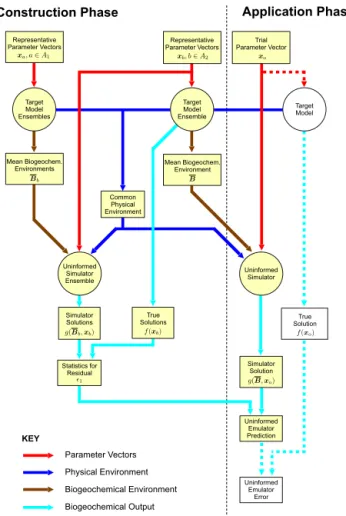
sample. A conceptual overview of the data flow in the emu-lator construction and evaluation process is given in Fig. 1.
The processing is divided into aconstruction phaseand an application phase. In a practical application, the construction phase is intended for single execution, whereas the applica-tion phase must be executed for each trial parameter vector. The procedure for assessment of the uninformed emulator against a known truth is shown as an extension to the appli-cation phase.
Error statistics must be determined using target model data that are independent from those used in the simulation. This means that, in the construction phase, target model ensemble members used to determineǫ1for the simulator output must
be different from those used to construct the mean environ-ment model for the simulator input. Furthermore, any tar-get model ensemble member used to assess the uninformed emulator performance must be different from any ensemble member used in the construction phase.
Target Model Ensembles
Target Model
Uninformed Simulator Ensemble
Uninformed Simulator Common
Physical Environment
Uninformed Emulator Prediction
Uninformed Emulator
Error Representative
Parameter Vectors
Parameter Vectors
Physical Environment
Biogeochemical Environment
Biogeochemical Output
KEY
Construction Phase Application Phase
Target Model Ensemble Representative Parameter Vectors
Trial Parameter Vector
Mean Biogeochem.
Environments Mean Biogeochem. Environment
True Solution
Simulator Solution Simulator
Solutions
True Solutions
B Bb
Statistics for Residual
!1
f(xb) f(xo)
g(B,xo) g(Bb,xb)
xa, a∈A1 xb, b∈A2 xo
Figure 1.Data flow for emulator construction and application to
the prediction of target model output where simulator uncertainty is quantified by the direct method.A1andA2are arbitrary sets of
indices satisfyingA1∩A2=∅. Simulation steps are indicated by circles. The dotted lines and uncoloured boxes indicate data flow for validating emulator performance against a known truth. They are not part of the practical application procedure, where the truth would be unknown.
simulation. The resulting contribution to simulation error is referred to as theparametric environment error. To define it, we consider a perfect simulatorgT(., .), such that
f (xo)=gT[BT(xo),xo], (9)
where BT is the complete and accurate description of the
local biogeochemical environment in the 3-D simulation, in-cluding advective and diffusive flux perturbations. The sim-ulator is perfect in the sense that it exactly reproduces the results of the 3-D simulation. Introducing parametric uncer-tainty in the biogeochemical environment and representing the environment by its expectation then gives
f (xo)=gT{E[BT(x)],xo} +ǫB:x∈χ , (10)
whereǫBis a stochastic residual, possibly with a non-zero
mean. This is the negated parametric environment error or parametric environment residual.
It is important to note that many different designs are pos-sible for a perfect simulator satisfying Eq. (9), having differ-ent formulations for concdiffer-entration dependency in the flux di-vergence tendencies. Variants of the applied perturbationP⋆
will give different results for the simulator term in Eq. (10), where the environment is not consistent with the simulation state, and therefore different residuals. The parametric envi-ronment error is therefore not just a property of the target model but depends also on the simulator design.
Combining Eqs. (8) and (10), the residual for the target model output with respect to the uninformed simulator out-put can be expressed as
ǫ1=ǫS+ǫB, (11)
whereǫSis a stochastic residual given by
ǫS=gT{E[BT(x)],xo} −g B,xo. (12)
ǫS is the departure of the hypothetical output of the perfect
simulator with the true mean environment from the output of the uninformed simulator. The first term describes a per-fectmean environment simulation, while the second term de-scribed its approximation by the simulator. In this context, we can refer to the uninformed simulator as a mean envi-ronment simulator. We refer toǫSas the mean environment
simulation residual. Mean environment simulation error (the negated residual) is caused by basic simulation errors that are not associated with parametric uncertainty in the envi-ronment.
It is not possible to evaluate the perfect simulator term in Eq. (12) and directly determine values forǫS. However, we
can get a handle on the impact of basic simulation errors from analysing the informed simulator. The relationship between the target model output forxoand that of the corresponding
informed simulator is given by
f (xo)=g[B(xo),xo] +ǫ2, (13)
whereB(xo)is the environment data derived from 3-D
sim-ulation output forxoandǫ2is a stochastic residual, possibly
having non-zero mean, referred to as theinformed simulator residual. Its negated value is theinformed simulator error.
The residualsǫ2andǫSare closely related, in that the input
B(xo)in the informed simulator is intended to approximate
the true parameter-specific environment in the same way that
Bin the uninformed simulator (or mean environment simu-lator) is intended to approximate the perfect simulator input E[BT(x)]. Both residuals are affected by basic simulation
er-rors. The difference is that the environment in Eq. (12) is not specific to the parameter vectorxo.
be greater than in the informed simulator. The mean envi-ronment simulation residualǫSmay therefore be more
sen-sitive to the concentration-dependency formulation than the informed simulator residual ǫ2. Nevertheless, to modelǫS
we make the pragmatic assumption that it is identically dis-tributed toǫ2. Statistics forǫ2are determined by direct
com-parison of informed simulator output with true output records from the target model.
The model for the parametric environment residualǫBis
derived from a parametric uncertainty analysis, following Hemmings and Challenor (2012). The environment corre-sponding to the trial parameter vector is unknown so we examine the distribution of the residual over many possible environments, aiming to achieve adequate coverage of the environment space that maps to the parameter space of in-terest. The method involves running a 1-D ensemble simula-tion based on a sample of environment realizasimula-tions. These are generated using the mean environment model and stochastic environment generator introduced in Sect. 2.2.
The environment generator uses independent statistical models for generating the initial state and the input flux per-turbations. For each of these two data sets, separate multi-variate Gaussian models are constructed using empirical or-thogonal functions (EOFs) that capture the dominant modes of variability in the target model ensemble output at each site. The statistical models for the initial state preserve spa-tial covariances (in the vertical) and covariances between the biogeochemical properties, as characterized by the first five EOFs of the sample anomalies, anomalies being determined with respect to the ensemble means. The statistical models for the advective flux perturbations preserve temporal and spatial covariances and covariances between the eight pri-mary tracers, again as characterized by the first five EOFs of the anomalies.
To derive the statistical model for a simulator’s initial state from a target model ensemble of sizen, ann×mmatrixY3d
is constructed containing thenavailable instances of the ini-tial state, as defined by the alternative state vectorS. (mis the number of elements inS.) Ify·j is the mean andsj2the variance of thejth column ofY3d, then the matrixZ3dwith
elements
zij=
yij−y·j
sj
(14) is the normalized form of Y3d for which each column has
zero mean and unit variance.
The environment generator uses the eigenvalues and eigenvectors obtained from the spectral decomposition of the correlation matrix forZ3d:
6= 1
n−1Z
T
3dZ3d=VT3V. (15)
3is a diagonal matrix with diagonal elementsλ1≥λ2. . .≥
λmcontaining the eigenvalues of6. Rows ofVare the cor-responding eigenvectors.
A data set containingNrealizations of the alternative state vector is generated by
Z1d=Q13
1 2
pVp
+Q2diag
q
1−vT13pv1, . . .,
q
1−vT
m3pvm
, (16)
where the subscriptpis used to indicate the firstprows and columns of3and rows ofVandvi is theith column ofVp. (Herep=5.)Q1is anN×pmatrix of random values andQ2
is anN×mmatrix of random values. The random variates are independent and normally distributed with zero mean and unit variance.Z1dis back-transformed (re-arranging Eq. 14)
to obtain anN×mmatrix containingN realizations of the state vectorS(to)for the 1-D environment ensemble. The
same analysis is applied to then available instances of the advective flux perturbation vectors from the 3-D ensemble to generateNrealizations of theP⋆vector.
Each of the N randomly generated environment realiza-tions is used to provide a separate estimate of the parametric environment residual corresponding to a possible truth. For theith ensemble member this is
ǫBi=g(Bi,xo)−g B,xo, (17)
whereBiis theith environment realization generated by the environment model. For the true environment,Bi would be
B(xo), as in the informed simulator. The environment
resid-ual statistics var(ǫB)and E(ǫB)are approximated by var(ǫBi) and E(ǫBi):i∈ {1, . . ., N}. In Eq. (17), we rely on the sim-ulatorg(., .) to provide estimates for the terms f (xo) and
gT(E[BT(x)],xo)in Eq. (10). Thus, the estimated
environ-ment residual statistics are to some extent affected by basic simulation errors and will not be strictly independent of the statistics for the mean environment simulation residualǫS.
It should be noted that the residualǫB and its predicted
distribution are dependent on the trial parameter vectorxo.
Hemmings and Challenor (2012) demonstrated that the de-pendency of environment error variance estimates on varia-tions in the simulation trajectory over the parameter space is potentially important in the context of a parametric analysis. For this reason, estimation of the environment residual statis-tics must be performed for each trial parameter vector in the analysis, so is a significant overhead.
If the underlying distributions of the residualsǫS andǫB
are taken to be Gaussian then they are fully described by their means and variances. Statistics for the uninformed simulator residualǫ1are obtained under the assumption thatǫSandǫB
can be considered only weakly dependent such that
E(ǫ1)=E(ǫS)+E(ǫB) (18)
and
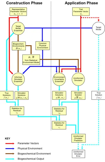
Target Model Ensemble
Target Model
Informed Simulator Ensemble
Environment Uncertainty Ensemble
Uninformed Simulator Biogeochem.
Environments
Uninformed Emulator
Error Representative
Parameter Vectors
Parameter Vectors
Physical Environment
Biogeochemical Environment
Biogeochemical Output KEY
Construction Phase Application Phase
Trial Parameter Vector
True Solutions
Simulator Solutions
Simulator Solutions
Simulator Solution
True Solution
Uninformed Emulator Prediction Common
Physical Environment
Statistics for Residual
xa, a∈A xo
from Statistical Environment Model
Bi,B
f(xa) g(Bi,xo) g(B,xo) f(xo)
!S g[B(xa),xa]
B(xa)
!1 Statistics for
Residual Statistics for
Residual !B
Figure 2.Data flow for emulator construction and application to
the prediction of target model output where simulator uncertainty is quantified by the indirect method.Ais an arbitrary set of indices. Simulation steps are indicated by circles. The dotted lines and un-coloured boxes indicate data flow for validating emulator perfor-mance against a known truth. They are not part of the practical ap-plication procedure, where the truth would be unknown.
Any indirect dependency betweenǫSandǫBthat might arise
from their dependencies on the simulator design is ignored. The uninformed simulator statistics are determined by sub-stituting our estimates for the residual statistics for each er-ror component in Eqs. (18) and (19). In doing so, we also ignore potential dependency arising from the effect of basic simulation errors on var(ǫBi).
A conceptual overview of the data flow for the indirect method is given in Fig. 2. Once again, the processing is di-vided into a construction phase intended for single execution and an application phase to be applied with each trial parame-ter vector. The procedure for assessment of the uninformed emulator is included in the application phase.
3 Experimental method
Anticipating the use of satellite ocean colour data for model calibration, an emulator was constructed for the NEMO-MEDUSA surface chlorophyll output at an array of oceanic sites. The surface chlorophyll concentration is the sum of the surface level chlorophyll concentrations for the two phyto-plankton types. Data for defining the biogeochemical envi-ronment were provided by a 10-member reference ensemble of global 3-D simulations with the NEMO-MEDUSA tar-get model. For emulator assessment, the known “truth” for a given trial parameter vector is defined by chlorophyll out-put from a target model simulation with that parameter vec-tor.
3.1 1-D experimental framework
To provide a representative range of oceanic conditions for the experiments, 12 sites were selected, located on a merid-ional transect along 20◦W in the North Atlantic at 5◦ inter-vals from 5 to 60◦N. This spans the sub-tropical gyre and temperate regions further north where large spring blooms are typical, extending into the sub-polar gyre south of Ice-land. To the south, it also crosses a high productivity region off the East African coast between the shelf break and the Cape Verde Islands.
Physical forcing data for the 1-D experiments, in the form of vertical velocitywp, the vertical diffusion coefficientKρ and temperature are taken from 5-day mean output common to all of the 3-D NEMO-MEDUSA simulations. Five-day mean time series of downwelling solar radiation at the sea surface and the soluble iron flux from dust deposition are likewise taken from 5-day data common to all reference sim-ulations.
Biogeochemical environment vectors for the 1-D experi-ments are based on initial state vectors and applied perturba-tion vectors from one or more 3-D simulaperturba-tions. Initial con-centrations are taken from NEMO-MEDUSA restart files. Approximate values for the applied perturbationp⋆ are de-rived from the target model’s 5-day mean current vector and primary tracer concentration fields using Eq. (7).
introducing an anomalous divergence in the vertical flow but the effect on the overall simulation is negligible. The upper ocean levels have boundaries at depths 6, 12, 19, 25, 32, 39, 46, 54, 62, 71, 80, 90, 100, 112, 124, 137, 152, 168, 187, 207, 229, 254, 281, 312, 347, 386, 429, 477, 531, 591, 656, 729, 809, 896, 991 and 1093 m.
The schemes used for vertical tracer transport are the same as those used in the target model and are described by Madec (2008). The diffusion scheme is an implicit scheme and the advection scheme is the Monotonic Upstream Scheme for Conservative Laws (Van Leer, 1977; Hourdin and Armen-gaud, 1999), introduced into NEMO for use in biogeochem-ical modelling studies by Lévy et al. (2001). A 1 h forward Euler time step is used.
3.2 Model parameter space
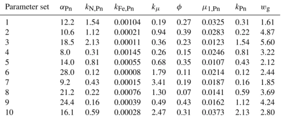
Full details of the derivation of the parameter space for the emulation experiments are given in Appendix A. Initially, a 28-dimensional parameter space of interest was defined; 28 parameters of particular relevance to the seasonal plank-ton dynamics in the upper ocean were selected from a set of 60 potential input parameters in the MarMOT 1.1 imple-mentation of MEDUSA. The parameter bounds were defined according to a set of rules designed to ensure that parame-ter values within the bounds are biologically plausible with respect to their defined roles.
The set of adjustable input parameters differs from the set of internal model parameters defined by Yool et al. (2011) due to a number of modifications made to facilitate paramet-ric analyses. For example, where pairs of parameters such as rate parameters are used in the model for the two differ-ent phytoplankton types, the diatom parameter has been re-placed in the input vector by the ratio of the two internal pa-rameters. The input non-diatom parameter then scales both of the internal phytoplankton parameter values without af-fecting their relationship, while the new input parameter con-trols the relationship. The zooplankton parameters are treated similarly. The changes allow us to consider the effects of a phytoplankton rate parameter or a zooplankton rate parame-ter on the system without having to consider the impact of directly changing the relationship between rates for closely related plankton types. It is then easier to interpret parameter effects at a high level of abstraction which facilitates compar-ison with simpler models where parameters represent rates for more aggregated plankton compartments.
The dimensionality of the initial parameter space was re-duced further with reference to a sensitivity analysis, per-formed at the experimental sites, to identify parameters that are influential with respect to annual primary production and sinking particle flux outputs from the model (see Ap-pendix A). Improving the reliability of these outputs in the target model will be important for understanding and pre-dicting change in the global carbon cycle. Eight model
pa-rameters were chosen on the basis of the findings. The corre-sponding parameter space is defined by Table 1.
One finding of the sensitivity analysis was that the input parameters controlling the relationship between associated internal parameters for different plankton types were less in-fluential than the input parameters exerting control over the different plankton types jointly. None of the input parame-ters from the first set were selected. The mapping of input parameters to internal parameters means that varying any of the five non-diatom phytoplankton parameters in Table 1 will also change the corresponding internal diatom parameters in proportion. The non-diatom density-independent loss rate and half-saturation concentration for density-dependent loss will additionally affect the corresponding internal parameters for both zooplankton types in proportion and the microzoo-plankton grazing half-saturation concentration will affect the corresponding internal parameter for mesozooplankton in the same way.
3.3 3-D reference simulations
A 10-member ensemble of 3-D simulations was used to cre-ate a reference sample of NEMO-MEDUSA output data that is representative of variability in the target model solution over the defined parameter space. The 10 parameter vectors are distributed in parameter space according to a Latin hyper-cube design (McKay et al., 1979). For improved coverage, a “maximin” criterion (Johnson et al., 1990) was applied to 1000 randomly generated hypercubes: the hypercube design is selected that maximizes the smallest Euclidean distance between parameter vector pairs in terms of their positions on a parameter space grid with an equal number of intervals in each dimension. Grid intervals are in log units for rate pa-rameters and half-saturation concentrations.
The chosen parameter vectors are given in Table 2. NEMO-MEDUSA integrations were performed for each of the 10 parameter vectors to provide representative output for a 2-year period, beginning in 1997. The second year, 1998, is the first complete year for which satellite ocean colour data from the SeaWiFS sensor are available (although these data are not used in the present study). The integrations, at 1◦ horizontal resolution, were initialized from the NEMO-MEDUSA simulation of Yool et al. (2011) at the beginning of 1995 and integrated for 4 years with their respective modi-fied parameter sets, thereby allowing a 2-year spin-up period prior to any analysis to attenuate the worst effects of tran-sient behaviour with respect to the seasonal cycle in the upper ocean. A longer spin-up time would normally be envisaged for a practical application, consistent with the intended use of the target model.
parameter-Table 1.8-dimensional MEDUSA parameter space for target model emulation.
Parameter Description and units Lower bound Upper bound
αPn chlorophyll-specific initial slope of P-I curve for non-diatoms
g C(g chl)−1(W m−2)−1d−1
7.5 30
kN,Pn N nutrient uptake half-saturation concentration for non-diatoms
mmol N m−3
0.1 2.5
kFe,Pn Fe nutrient uptake half-saturation concentration for
non-diatoms mmol Fe m−3
0.000066 0.0017
kµ microzooplankton grazing half-saturation concentration
mmol N m−3
0.16 4
φ zooplankton grazing inefficiency
–
0.05 0.45
µ1,Pn non-diatom phytoplankton density-independent loss rate
d−1
0.01 0.04
kPn non-diatom phytoplankton half-saturation concentration for
density-dependent loss mmol N m−3
0.1 2.5
wg detrital sinking rate
m d−1
1.5 6
Table 2.Representative sample from 8-dimensional MEDUSA parameter space.
Parameter set αPn kN,Pn kFe,Pn kµ φ µ1,Pn kPn wg
1 12.2 1.54 0.00104 0.19 0.27 0.0325 0.31 1.61
2 10.6 1.12 0.00021 0.94 0.39 0.0283 0.22 4.87
3 18.5 2.13 0.00011 0.36 0.23 0.0123 1.54 5.60
4 8.0 0.31 0.00145 0.26 0.15 0.0246 0.81 3.22
5 14.0 0.81 0.00055 0.68 0.35 0.0107 0.43 2.12
6 28.0 0.12 0.00008 1.79 0.11 0.0214 0.12 2.44
7 9.2 0.43 0.00015 3.41 0.19 0.0187 0.16 1.85
8 21.2 0.22 0.00076 1.30 0.07 0.0141 0.59 3.69
9 24.4 0.16 0.00039 0.49 0.43 0.0162 1.12 4.24
10 16.1 0.59 0.00028 2.47 0.31 0.0373 2.13 2.80
specific environment information for 1-D simulator construc-tion.
3.4 Emulator construction and assessment
Performance of the basic 1-D simulator array is evaluated, with respect to surface chlorophyll, for a set of trial parame-ter vectors for which the true target model output is known. The performance of emulators constructed using the two un-certainty quantification methods is then assessed. Finally, to explore the importance of the lateral flux perturbations, we assess the performance of simulator arrays in which these are omitted. In this context, the behaviour of an alternative array employing informed simulators is examined in addition to that of the uninformed simulator array used in the emulator. Doing this allows us to see the impact of omitting lateral flux perturbations in a scenario where other error sources are
min-imized. The experimental methods for the assessments are as follows.
3.4.1 Simulator assessment
Informed simulator skill is described by error statistics cal-culated from a set of 10 experiments with the representative parameter vectors defined in Table 2, so that each experiment corresponds to one of the available 3-D reference simula-tions. In each experiment, the informed simulator is initial-ized at the start of 1997 and run for 2 years. If the set of repre-sentative parameter vectors is denoted byX= {x1, . . .,x10},
then the trial parameter vector for theith experiment isxi and the environment is defined by the 3-D ensemble member with parameter vectorxi.
covering the same time period. One experiment was per-formed for each parameter vector in X but simulator con-struction was performed on a leave-one-out basis: in theith experiment, the trial parameter vector isxi and the mean vironment is derived from the nine NEMO-MEDUSA en-semble members with x6=xi, x∈X, leaving the NEMO-MEDUSA outputf (xi)as independent data for validation. Thus, each experiment uses a slightly different version of the simulator, constructed by applying the same method to a dif-ferent nine-member ensemble.
Error statistics are calculated with respect to the log-transformed 5-day mean chlorophyll output. The log trans-formation applied to the 5-day means acts to stabilize the er-ror variance which otherwise tends to increase with increas-ing chlorophyll concentration. Its use in the analysis of sur-face chlorophyll variability is strongly supported by theoret-ical considerations and empirtheoret-ical data (Campbell, 1995). 3.4.2 Assessment of the full emulator
Validation of the complete uninformed emulator for surface chlorophyll is by analysis of the results from the 10 leave-one-out experiments, taking into account the predicted sim-ulator error statistics to determine the emsim-ulator robustness. These uncertainty estimates are, like the simulator itself, re-quired to be independent of parameter-specific environment information. Thus, for the ith experiment, they are derived using the nine NEMO-MEDUSA ensemble members with
x6=xi. The uninformed emulator uncertainty is quantified using the direct and indirect methods.
When the indirect method is used, the nine NEMO-MEDUSA ensemble members are used to derive statistics for the two component residualsǫSandǫB. In the estimation of
the statistics for the mean environment simulation residual
ǫS (assumed identically distributed to the informed
simula-tor residualǫ2), the 3-D ensemble members are required for
comparison with the corresponding informed simulators to determine informed simulator error. In the estimation of the statistics for the parametric environment residualǫB, the
3-D ensemble is required for building the environment model used in the parametric uncertainty analysis.
When the direct method is used, the nine NEMO-MEDUSA ensemble members are used to derive statistics for the uninformed simulator residualǫ1. Each of the nine
cor-responding uninformed simulators require independent data for their mean environment input. In theith experiment, the mean environment for the uninformed simulator with para-meter vectorxj is derived from the eight NEMO-MEDUSA members withx6=xi∩x6=xj. As a result, simulators must be constructed with 90 different mean environment estimates to calculate the uncertainty estimates for the 10 experiments. For the uncertainty quantification analyses, Gaussian error distributions in log-transformed chlorophyll are assumed so that the resulting probability density functions for the resid-uals are fully described by their mean and variance, both of
which are allowed to vary in time and between sites. The residuals are defined with respect to log-transformed 5-day mean chlorophyll concentrations. Their predicted distribu-tions are described by their monthly means and variances, interpolated to 5-day intervals. Appendix B gives the estima-tion method for the residual statistics and the resulting time series.
4 Results
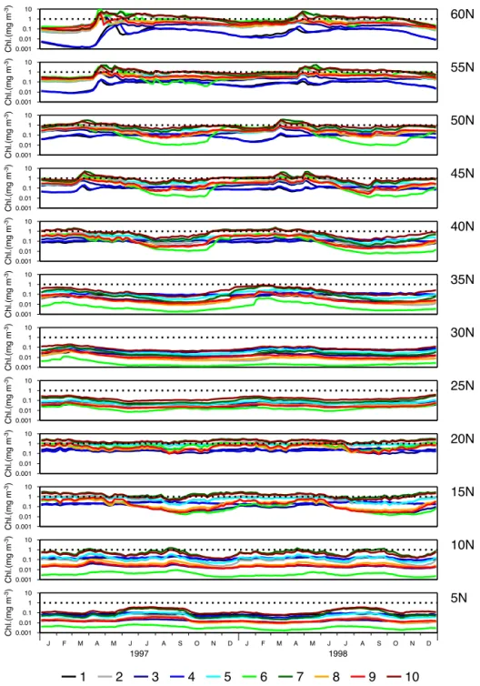
The surface chlorophyll records from the 3-D NEMO-MEDUSA reference ensemble at each of the experimental sites are shown in Fig. 3. This shows the spatial variation in chlorophyll from values a little above 0.001 mg m−3 in the
oligotrophic gyre at 30 and 35◦N for Parameter Set 6 to
sea-sonal highs associated with the spring bloom in temperate regions (45–60◦N), approaching 10 mg m−3for a number of the parameter vectors. It also illustrates the variability in the seasonal response of the plankton dynamics which is gener-ally stronger at the more northerly sites.
The variation between records produced by different pa-rameter vectors is large compared with the seasonal vari-ability. At some sites, particularly 5–10◦N and 25–35◦N, the parameter dependency manifests primarily as a control on the overall chlorophyll concentration level in the surface layer, throughout the annual cycles. These are generally the more oligotrophic sites, where concentrations remain below or very close to 1 mg m−3for all parameter vectors. At other sites, particularly in the north, the different parameters also have a notable influence on the dynamic range and there is some evidence of an impact on the characteristics of the spring bloom.
Some parameter vectors tend to have the same effect on overall surface chlorophyll levels at all sites. For example, Parameter Set 10 gives elevated levels over the whole data set. However, this is not generally the case. Parameter Set 6, for example, shows a strong tendency to give low chloro-phyll concentrations at many of the sites but gives some of the higher concentrations at 55 and 60◦N. With this para-meter vector, the phytoplankton light-response controlled by
αPnis exceptionally strong and nutrient-limitation is reduced
by low half-saturation concentrationskN,Pn andkFe,Pn. As a
result, the phytoplankton can achieve very high growth rates. This can cause blooms that lead to long-term nutrient de-pletion as a consequence of organic material sinking out of the euphotic zone. Subsequent growth is then inhibited. At four sites (5, 10, 30 and 35◦N), nitrogen depletion during the 2-year spin-up period results in very low chlorophyll con-centrations at the start of 1997 which remain relatively low throughout 1997 and 1998.
0.001 0.01 0.1 1 10
Chl.(mg m
-3) 60N
0.001 0.01 0.1 1 10
Chl.(mg m
-3) 55N
0.001 0.01 0.1 1 10
Chl.(mg m
-3) 50N
0.001 0.01 0.1 1 10
Chl.(mg m
-3) 45N
0.001 0.01 0.1 1 10
Chl.(mg m
-3) 40N
0.001 0.01 0.1 1 10
Chl.(mg m
-3) 35N
0.001 0.01 0.1 1 10
Chl.(mg m
-3) 30N
0.001 0.01 0.1 1 10
Chl.(mg m
-3) 25N
0.001 0.01 0.1 1 10
Chl.(mg m
-3)
20N
0.001 0.01 0.1 1 10
Chl.(mg m
-3) 15N
0.001 0.01 0.1 1 10
Chl.(mg m
-3) 10N
0.001 0.01 0.1 1 10
J F M A M J J A S O N D J F M A M J J A S O N D
1997 1998
Chl.(mg m
-3) 5N
1 2 3 4 5 6 7 8 9 10
Figure 3.Five-day mean surface chlorophyll output from 3-D NEMO-MEDUSA simulations for the 10 parameter vectors in Table 2, colour
coded by Parameter Set number.
the highest concentrations throughout 1997 and 1998 at the most southerly sites. These parameter vectors combine low
αPn values with low values for the grazing half-saturation
concentrationkµ, reducing phytoplankton production at low light levels and making them more susceptible to zooplank-ton grazing. This makes the phytoplankzooplank-ton less well-suited to over-wintering at the high latitude sites where light avail-ability is very low due to the combination of low surface ir-radiance and deep winter mixing.
The strong variation between parameter vectors indicates the potential for significant constraints on the parameter val-ues to be realized by the assimilation of satellite chlorophyll data.
4.1 Emulator prediction of target model output
0.0001 0.001 0.01 0.1 1 10
0.0001 0.001 0.01 0.1 1 10
NEMO-MEDUSA chlorophyll (mg m-3)
MarMOT-MEDUSA chlorophyll (mg m
-3)
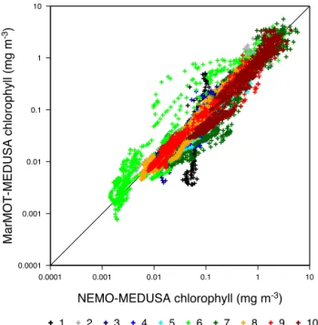
1 2 3 4 5 6 7 8 9 10
Figure 4.Five-day mean surface chlorophyll output for 1998 at all
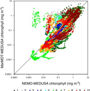
12 sites from the uninformed simulator, compared with that from the matching 3-D NEMO-MEDUSA reference simulation. Results are shown for the 10 different parameter vectors in Table 2, colour coded by Parameter Set number.
from the matching 3-D experiment in Fig. 4. Data are shown for the 1998 annual cycle only, so are representative of the simulator performance 1 year on from its initialization year, during which errors have had time to develop.
The correlation between simulator and target model val-ues is good. Pearson’s correlation coefficientrfor the simu-lator and target model output is 0.91, indicating that 83 % of the variance in the log-transformed surface chlorophyll from the simulator array is explained by the target model out-put. There are some notable examples of poor performance though. In particular, the results for Parameter Set 6 indicate a strong positive bias, with the simulator array overestimat-ing some surface chlorophyll values by an order of magni-tude. There are some fairly large negative biases for other parameter sets, notably Parameter Sets 7 and 10 at mid-range concentrations, although these are less systematic. Also, the simulator array poorly reproduces the relatively low variabil-ity in chlorophyll associated with Parameter Set 1.
The chlorophyll output from the uninformed emulator in-cludes a bias correction term which depends on the un-certainty quantification method. (This corrects for spatio-temporal biases rather than for parameter-related biases.) When using the direct uncertainty quantification method, the bias-corrected error in log-transformed 5-day mean chloro-phyll is
dUd=g B,xo+u1−f (xo), (20)
whereu1 is our estimate of E(ǫ1). When using the indirect
method, the bias correction includes corrections for both the mean environment simulation bias and the bias associated with parametric environment uncertainty. The bias-corrected error is then
dUi=g B,xo
+uS+uB(xo)−f (xo), (21)
whereuS anduB are our estimates of E(ǫS)and E(ǫB)
re-spectively andB is our estimate of the mean environment. The estimatesu1anduSwere determined without reference
to results for Parameter Set 6. These were excluded on the basis of the unrepresentative simulator performance, to avoid excessive influence from a single outlier. Time series ofu2
anduS are therefore based on an ensemble size of 8 (or 9,
when Parameter Set 6 is the trial parameter vector).
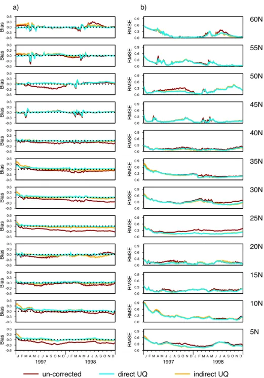
Error statistics for the uninformed emulator results are given in Fig. 5. Results are presented for the basic simula-tor array with no bias correction (u1=uS=uB=0) and for
the full emulator with bias correction. There are only minor differences between the mean and rms values for dUd and
dUi.
Biases are reduced by the emulator’s bias correction scheme, irrespective of the method used. Time series of sim-ulator bias before and after correction show that in both cases the bias correction is effective at all sites, with the possi-ble exception of 20◦N wheredUi shows the introduction of
a negative bias in the summer of 1998 when using the in-direct uncertainty quantification method. In particular, note that the summer 1998 bias at 60◦N is largely removed and
the correction is particularly effective in removing negative bias at some of the more oligotrophic sites (5 and 25–30◦N) and at 50◦N in 1997.
The relatively high rms errors for early 1997 at most sites are the consequence of transient behaviour associated with error in the initial conditions. This source of error seems to influence the model primarily in the early half of the year, before the local dynamics start to dominate over the environ-mental influence. The lack of parameter-specific information about the lateral fluxes appears to be a less dominant source of simulation error. Nevertheless, it does contribute strongly to the relatively large 1998 errors at 5 and at 50◦N.
4.2 Robustness of the emulator
-0.6 -0.3 0.0 0.3 0.6 Bias 0.0 0.3 0.6 0.9 RMSE 60N a) b) -0.6 -0.3 0.0 0.3 0.6 Bias 0.0 0.3 0.6 0.9 RMSE 55N -0.6 -0.3 0.0 0.3 0.6 Bias 0.0 0.3 0.6 0.9 RMSE 50N -0.6 -0.3 0.0 0.3 0.6 Bias 0.0 0.3 0.6 0.9 RMSE 45N -0.6 -0.3 0.0 0.3 0.6 Bias 0.0 0.3 0.6 0.9 RMSE 40N -0.6 -0.3 0.0 0.3 0.6 Bias 0.0 0.3 0.6 0.9 RMSE 35N -0.6 -0.3 0.0 0.3 0.6 Bias 0.0 0.3 0.6 0.9 RMSE 30N -0.6 -0.3 0.0 0.3 0.6 Bias 0.0 0.3 0.6 0.9 RMSE 25N -0.6 -0.3 0.0 0.3 0.6 Bias 0.0 0.3 0.6 0.9 RMSE 20N -0.6 -0.3 0.0 0.3 0.6 Bias 0.0 0.3 0.6 0.9 RMSE 15N -0.6 -0.3 0.0 0.3 0.6 Bias 0.0 0.3 0.6 0.9 RMSE 10N -0.6 -0.3 0.0 0.3 0.6
J F M A M J J A S O N D J F M A M J J A S O N D
1997 1998 Bias 0.0 0.3 0.6 0.9
J F M A M J J A S O N D J F M A M J J A S O N D
1997 1998
RMSE
5N
un-corrected direct UQ indirect UQ
Figure 5.Uninformed emulator error statistics for log10(surface chlorophyll) (mg m−3) over 10 experiments, one experiment for each of
the parameter vectors in Table 2:(a)bias and(b)rms error. The statistics are shown for the simulators without bias correction and for the bias-corrected simulator array, which is the uninformed emulator. The emulator statistics are given for emulator versions constructed using direct and indirect uncertainty quantification methods (i.e. for errorsdUdanddUi).
with zero mean and unit standard deviation at all times and locations.
The normalized uninformed emulator error for each log-transformed 5-day mean surface chlorophyll concentration depends on the uncertainty quantification method. For the di-rect method, it is given by
DUd=
g B,xo
+u1−f (xo)
s1
, (22)
wheres12is our estimate for var(ǫ1). For the indirect method,
it is
DUi=
g B,xo+uS+uB(xo)−f (xo)
q
sS2+sB2(xo)
, (23)
wheresS2andsB2are our estimates for var(ǫS)and var(ǫB)
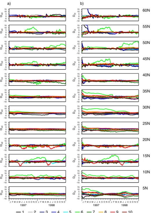
-10 -5 0 5 10 15 DUd -10 -5 0 5 10 15 DUi 60N a) b) -10 -5 0 5 10 15 DUd -10 -5 0 5 10 15 DUi 55N -10 -5 0 5 10 15 DUd -10 -5 0 5 10 15 DUi 50N -10 -5 0 5 10 15 DUd -10 -5 0 5 10 15 DUi 45N -10 -5 0 5 10 15 DUd -10 -5 0 5 10 15 DUi 40N -10 -5 0 5 10 15 DUd -10 -5 0 5 10 15 DUi 35N -10 -5 0 5 10 15 DUd -10 -5 0 5 10 15 DUi 30N -10 -5 0 5 10 15 DUd -10 -5 0 5 10 15 DUi 25N -10 -5 0 5 10 15 DUd -10 -5 0 5 10 15 DUi 20N -10 -5 0 5 10 15 DUd -10 -5 0 5 10 15 DUi 15N -10 -5 0 5 10 15 DUd -10 -5 0 5 10 15 DUi 10N -10 -5 0 5 10 15
J F M A M J J A S O N D J F M A M J J A S O N D
1997 1998 DUd -10 -5 0 5 10 15
J F M A M J J A S O N D J F M A M J J A S O N D
1997 1998
DUi
5N
1 2 3 4 5 6 7 8 9 10
Figure 6.Normalized uninformed emulator error for emulator versions constructed using(a)the direct uncertainty quantification method
(DUd) and(b)the indirect uncertainty quantification method (DUi). Errors are shown for the 10 different parameter vectors in Table 2, colour
coded by Parameter Set number. Off scaleDUivalues not shown at the beginning of 1997 go up to about 26 at 55◦N and about 35 at 60◦N.
uS, were determined without reference to the results for
Para-meter Set 6, so were likewise based on a sample size of eight (or nine when Parameter Set 6 is the trial parameter vector). The denominator in Eq. (22) varies between 0.014 and 0.62 log10units and that in Eq. (23) varies between 0.015 and 0.50 log10units (with chlorophyll concentration in mg m−3).
Fur-ther details of the residuals’ statistics and their variation in time and between sites can be found in Appendix B.
is not represented in the data used for emulator construction. Large normalized error values in Experiment 6 are therefore unsurprising.
When the indirect uncertainty quantification method is used, Fig. 6 shows that there are also very large extremes as-sociated with the post-initialization phase, particularly at 55 and 60◦N. These highDUivalues occur for experiments with
the two parameter vectors that were seen to cause unusu-ally low winter-time chlorophyll concentrations at the start of 1997 in the target simulation (Fig. 3, Parameter Sets 1 and 4). Fortunately, at these sites, the extreme error appears fairly transient, lasting only a few months. At other sites, in partic-ular at 5◦N,DUi remains correlated to some extent with its
early 1997 value over the whole 2-year period, suggesting that parametric error in the initial state may be introducing persistent biases. This pattern seems to be a common fea-ture of the more oligotrophic sites, being reflected also at latitudes from 25 to 35◦N. At more northerly sites, there is a tendency for persistent biases over long time periods where relatively large errors occur (e.g. at 45 and 50◦N for the indi-rect method) but this pattern develops later with no obvious connection to initialization error.
Comparing the two uncertainty quantification methods, it is seen that DUi initially tends to be larger thanDUd at all
sites. The post-initializationDUdvalues are more consistent
with their predicted distribution. In particular, the extreme positiveDUi values seen in early 1997 are not replicated in
DUd. From these observations, it is clear that the indirect
method is generally less effective at quantifying initial uncer-tainty. Furthermore, at the oligotrophic sites where the early 1997 biases tend to persist, there is a general tendency for
DUito be larger thanDUdover the 2-year period.
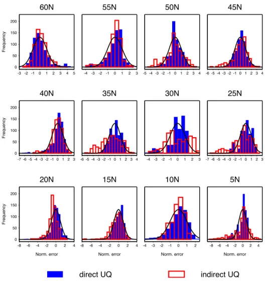
The normalized error distributions for the uninformed em-ulators are compared with the predicted distribution in Fig. 7. Results, including 1998 data only, are shown for each site. Experiment 6 is excluded to allow the results for the remain-ing experiments to be more clearly represented. The emula-tor with direct uncertainty quantification appears fairly ro-bust withDUddistributions broadly similar to the predicted
distribution at all sites. The worst performance is arguably at 30◦N where there are a significant proportion of anoma-lously low values associated with persistent negative errors in the experiments with Parameter Sets 1 and 4 (Fig. 6). How-ever,DUishows a strong tendency to be larger than expected
at a number of the sites. In general, these are the sites that have already been associated with persistent error in some of the experiments (5, 25–35, 45–50◦N). A smaller propor-tion of theDUdvalues at 15 and 20◦N are rather larger than
predicted. These are associated with extreme negative biases occurring in Experiment 9 that persist only for a month or two.
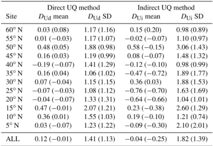
Table 3 summarizes the uninformed emulator results in terms of the mean and standard deviation of the normalized errors. Statistics are given for all 10 experiments combined and in brackets for the 9 experiments excluding Experiment
Table 3.Uninformed emulator robustness evaluation for all 10
ex-periments and for the 9 exex-periments excluding Experiment 6.
Direct UQ method Indirect UQ method Site DUdmean DUdSD DUimean DUiSD
60◦N 0.03 (0.08) 1.17 (1.16) 0.15 (0.20) 0.98 (0.89) 55◦N 0.01 (−0.03) 1.17 (1.07) −0.02 (−0.07) 1.10 (0.97) 50◦N 0.48 (0.05) 1.88 (0.98) 0.58 (−0.15) 3.06 (1.43) 45◦N 0.16 (0.03) 1.19 (0.99) 0.08 (−0.07) 1.48 (1.32) 40◦N −0.19 (−0.07) 1.41 (1.29) −0.12 (−0.10) 0.98 (0.99) 35◦N 0.16 (0.04) 1.06 (1.02) −0.47 (−0.72) 1.89 (1.77) 30◦N 0.07 (−0.04) 1.15 (1.15) 0.36 (0.03) 1.88 (1.53) 25◦N −0.07 (−0.03) 1.08 (1.12) −0.76 (−0.70) 1.63 (1.69) 20◦N −0.04 (−0.07) 1.33 (1.31) −0.64 (−0.66) 1.04 (1.01) 15◦N 0.47 (−0.01) 2.07 (1.21) 0.23 (−0.38) 2.60 (1.29) 10◦N 0.36 (0.01) 1.55 (1.03) 0.19 (−0.10) 1.21 (0.74) 5◦N 0.03 (−0.07) 1.23 (1.22) −0.09 (−0.30) 2.10 (2.01) ALL 0.12 (−0.01) 1.41 (1.13) −0.04 (−0.25) 1.82 (1.39)
6. The difference between the two sets of results illustrates to some extent the sensitivity of the evaluation statistics to sampling error.
When the emulator performance with direct uncertainty quantification is evaluated over all experiments and all sites, theDUd standard deviation is rather high at 1.41,
suggest-ing that the emulator is a little over-confident. When Exper-iment 6 is excluded from the evaluation, the standard devia-tion drops to 1.13. Whether or not this is a more appropriate measure of performance depends on the extent to which the model dynamics with Parameter Set 6 are representative of its behaviour over a significant region of parameter space. The performance with respect to the other parameter vectors is fairly reliable at all sites, with standard deviations from 0.98 to 1.31 and very little sign of post-correction bias shown byDUdmean values. All but two of the standard deviations
are above 1, indicating a slight tendency for the spread of the simulator residuals to be under-estimated. When Experi-ment 6 results are included in the evaluation data set, this ten-dency for over-confidence is more evident and there are no-table positive biases at a number of sites (DUdmean greater
than 0.3 at 10, 15 and 50◦N). These are associated with rel-atively largeDUdstandard deviations (1.55 to 2.07).
The high standard deviation inDUi of 1.82 is consistent