Assessment of heat sources on the control of fast flow of Vestfonna Ice Cap, Svalbard

(1)

TCD

7, 5097–5145, 2013

Heat production sources and dynamics of VSF

M. Schäfer et al.

Title Page

Abstract Introduction

Conclusions References

Tables Figures

◭ ◮

Back Close

Full Screen / Esc

Printer-friendly Version Interactive Discussion

Discussion

P

a

per

|

D

iscussion

P

a

per

|

Discussion

P

a

per

|

Discuss

ion

P

a

per

The Cryosphere Discuss., 7, 5097–5145, 2013 www.the-cryosphere-discuss.net/7/5097/2013/ doi:10.5194/tcd-7-5097-2013

Open Access

The Cryosphere

Discussions

This discussion paper is/has been under review for the journal The Cryosphere (TC). Please refer to the corresponding final paper in TC if available.

Assessment of heat sources on the

control of fast flow of Vestfonna Ice Cap,

Svalbard

M. Schäfer1, F. Gillet-Chaulet2, R. Gladstone1, R. Pettersson3, V. A. Pohjola3, T. Strozzi4, and T. Zwinger5

1

Arctic Centre, University of Lapland, Rovaniemi, Finland 2

Laboratoire de Glaciologie et Géophysique de l’Environment (LGGE), UMR5183, UJF-Grenoble 1, CNRS, Grenoble, France

3

Department of Earth Sciences, Air, Water and Landscape science, Uppsala University, Uppsala, Sweden

4

Gamma Remote Sensing and Consulting AG, Gümligen, Switzerland 5

CSC – IT Center for Science Ltd., Espoo, Finland

Received: 8 September 2013 – Accepted: 22 September 2013 – Published: 15 October 2013

Correspondence to: M. Schäfer ([email protected])

(2)

TCD

7, 5097–5145, 2013

M. Schäfer et al.

Title Page

Tables Figures

◭ ◮

Back Close

Full Screen / Esc

Discussion

P

a

per

|

D

iscussion

P

a

per

|

Discussion

P

a

per

|

Discuss

ion

P

a

per

Abstract

The dynamic regime of Svalbard’s Nordaustlandet ice caps is dominated by fast flow-ing outlet glaciers, makflow-ing assessment of their response to climate change challengflow-ing. A key element of the challenge lies in the fact that the motion of fast outlet glaciers oc-curs largely through basal sliding, and is governed by physical processes at the glacier

5

bed, processes that are difficult both to observe and to simulate. Up to now, most of the sliding laws used in ice flow models were based on uniform parameters with a condition on temperature to identify regions of basal sliding. However these models are usually not able to reproduce observed velocities with sufficient accuracy. With the develop-ment of inverse methods, it is now common to infer a spatially varying field of sliding

10

parameters from surface ice-velocity observations. These parameter distributions usu-ally reflect a high spatial variability and represent valuable information to understand and test various hypotheses on physical processes involved in sliding. However, in these models, basal sliding is uncoupled from the thermal regime of basal ice and the evolution of the sliding parameters in prognostic simulations remains problematic.

15

Here we explore the role of different heat sources (friction heating, strain heating and latent heat through percolation of melt water) on the development of sliding and fast flow through thermomechanical coupling on Nordaustlandet outlet glaciers. We focus on Vestfonna with a special emphasis on Franklinbreen, a fast flowing outlet glacier which has been observed to accelerate between 1995 and 2008 and possibly already

20

prior to 1995. We try to reconcile the impacts of temperature and heat sources on basal friction coefficients inferred from observed surface velocities during these two periods. Our simulations reproduce a temperature profile from borehole measurements, al-lowing an interpretation of the vertical temperature structure in terms of temporal evo-lution of climate. We identify firn heating as a crucial heat source to explain Vestfonna’s

25

(3)

TCD

7, 5097–5145, 2013

M. Schäfer et al.

Title Page

Tables Figures

◭ ◮

Back Close

Full Screen / Esc

Discussion

P

a

per

|

D

iscussion

P

a

per

|

Discussion

P

a

per

|

Discuss

ion

P

a

per

that hydrology and/or sediment physics need to be represented in order to simulate fast flowing outlet glaciers.

1 Introduction

Recent studies suggest that contributions to sea level change over the coming decades will be dominated by cryospheric mass loss in the form of discharge from fast flowing

5

ice streams or outlet glaciers (Meier et al., 2007; Moon et al., 2012; Jacob et al., 2012; Tidewater Glacier Workshop Report, 2013). Therefore, understanding the response of fast flowing features to changing climate is crucial in order to make reliable projections (Moore et al., 2011; Rignot et al., 2011; Shepherd et al., 2012; Dunse et al., 2012).

Observations dating back several decades show multiple modes of fast ice flow

be-10

havior including permanently fast flowing outlet glaciers or ice streams, networks of ice streams that switch between fast and slow flow (Boulton and Jones, 1979), pulsing glaciers (Mayo, 1978), natural variability in fast flowing outlet glaciers (Iken, 1981), and surging glaciers that show occasional massive accelerations from a more or less stag-nant state. Given that the underlying processes behind this range of features are not

15

yet fully understood, and may show significant overlap, we do not limit consideration to a subset of these possible fast flow behaviors. In the current study, we use the termfast flow featureto describe a glacier or ice stream that is capable of flowing significantly faster than can be accounted for by internal deformation – even close to pressure melt-ing point, i.e. that undergoes some form of basal slidmelt-ing. Note that bybasal slidingwe

20

mean non-zero ice velocity at the bed, which could be caused by sliding over the bed and/or deformation of underlying sediment.

We focus our study on the fast flow features of the Vestfonna ice cap. Austfonna and Vestfonna are the two major ice caps of Nordaustlandet, the second largest island of Svalbard, an Arctic archipelago located at around 80◦N. Vestfonna covers about

25

(4)

TCD

7, 5097–5145, 2013

M. Schäfer et al.

Title Page

Tables Figures

◭ ◮

Back Close

Full Screen / Esc

Discussion

P

a

per

|

D

iscussion

P

a

per

|

Discussion

P

a

per

|

Discuss

ion

P

a

per

interior ice. It is instead dominated by fast flowing outlet glaciers that extend from the coast to close to the ice divide. All the fast outlet glaciers on Vestfonna are thought to be topographically controlled (Pohjola et al., 2011). Many Svalbard glaciers are of surge-type, typically with a quiescent phase of∼100 yr, a surge phase of a few years, and an acceleration during the surge of factor 10 or higher. Svalbard surge mechanisms have

5

often been associated with thermal instabilities (Payne and Dongelmans, 1997; Murray et al., 2000; Fowler et al., 2001, 2010). However, such mechanisms are criticized due to their inability to explain surges of temperate (Alaskan type) glaciers (Murray et al., 2000; Fowler et al., 2001), which are suspected to be mainly hydrologically controlled (Murray et al., 2003). Murray et al. (2003) suggest that at least two different surge

10

mechanisms exist specific to temperate and polythermal glaciers. However, Sund et al. (2009) showed that surges in polythermal glaciers may also be initiated above the melt-freeze boundary on the glacier, raising the possibility of a single surge mechanism for both polythermal and temperate glaciers in which the surge is initiated in the temperate part (Sund et al., 2011).

15

Although thermomechanical control of ice deformation is relatively well understood today (Payne et al., 2000), the physical processes controlling basal sliding, which have been subject to some investigation (Kamb, 2001), remain to be better understood. Many processes and feedbacks have been suggested, including sub-glacial hydrol-ogy (Kamb, 1987; Vaughan et al., 2008; Bougamont et al., 2011; van der Wel et al.,

20

2013), deformation of sub-glacial sediments (Tru_ffer et al., 2000), heat gain from slid-ing (friction heatslid-ing) (Fowler et al., 2001; Price et al., 2008), from strain heatslid-ing (Clarke et al., 1977; Pohjola and Hedfors, 2003; Schoof, 2004) or thermal instabilities (Mur-ray et al., 2000). Payne and Dongelmans (1997) show that streaming flow can arise solely as a consequence of coupled flow and temperature evolution. However, while

25

(5)

TCD

7, 5097–5145, 2013

M. Schäfer et al.

Title Page

Tables Figures

◭ ◮

Back Close

Full Screen / Esc

Discussion

P

a

per

|

D

iscussion

P

a

per

|

Discussion

P

a

per

|

Discuss

ion

P

a

per

basal sliding requires the presence of liquid water and thus temperate conditions for the basal ice. Sliding also plays an important role in the thermal regime of the ice due to its impacts on heat advection and heat generation due to friction at the bed.

Basal sliding in ice flow models is typically described by a friction law where the in-situ complexity is represented by a few free parameters. Many large scale flow models

5

use spatially uniform parameters for the friction law but only allow sliding when ice at the bed reaches the pressure melting point (Greve, 1997; Ritz et al., 2001; Quiquet et al., 2013). This method does not allow accurate reproduction of spatial patterns in observed surface velocities with great fidelity. With the recent development of inverse methods, some modeling studies now constrain spatially varying friction law

param-10

eters to obtain the best match between model and observed surface velocities. This approach allows quantification of the basal sliding velocity which can help to constrain the in-situ processes (Morlighem et al., 2010; Pralong and Gudmundsson, 2011; Jay-Allemand et al., 2011; Habermann et al., 2012). However, this approach allows neither a relationship between friction and temperature nor time evolution of the friction

param-15

eter.

Here, we use a combination of modeling, field, and remote observations to study links between the thermal regime, heat sources and basal sliding in the Vestfonna fast flow features, especially during the recent speed-up of Franklinbreen (Pohjola et al., 2011), a major outlet glacier on Vestfonna. The research area and observational data

20

have been presented in detail by Schäfer et al. (2012). Key features and additional data are described in Sect. 2. We use the Elmer/Ice finite element Full Stokes ice dynamic model to simulate ice flow and to solve the inverse problem to constrain basal sliding from the observations (Sect. 3). After the model initialization, we assess the influence of the different heat sources on the temperature distribution: friction heating (due to

25

(6)

feed-TCD

7, 5097–5145, 2013

M. Schäfer et al.

Title Page

Tables Figures

◭ ◮

Back Close

Full Screen / Esc

Discussion

P

a

per

|

D

iscussion

P

a

per

|

Discussion

P

a

per

|

Discuss

ion

P

a

per

backs between basal sliding and the thermal regime are discussed in Sect. 5 before we conclude in Sect. 6.

2 Research area and observational data

Vestfonna (VSF) is characterized by a varied topography with two main ridges and strongly pronounced fast outlet glaciers. In common with most glaciers in Svalbard

5

VSF is polythermal. VSF was the target of a recent International Geophysical Year (IPY) project (Pohjola et al., 2011), and the observational record extends back to IPY 1957–1958 (Schytt, 1964) when data on surface elevation (using barometer methods) and ice thickness (from seismic surveys) were gathered. One focus of this work is Franklinbreen, the largest outlet glacier, which is situated on the northwestern side of

10

the ice cap and has recently accelerated (Pohjola et al., 2011; Braun et al., 2011).

2.1 Digital elevation models of surface and bedrock topography

For surface elevation the topographic map from the Norwegian Polar Institute (NPI) is used (1 : 100 000, 1990). This is based on aerial photography and completed with the International Bathymetric Chart of the Arctic Ocean (IBCAO Jakobsson et al., 2008)

15

in the sea. The coordinate is in UTM zone 33N, with datum WGS 1984. The bedrock data is a combination of ground-based pulsed radar and airborne radio-echo soundings (Pettersson et al., 2011). The ground-based radar was deployed only in the central part, for safety reasons. The airborne radar did not give good bedrock depth in the thicker central area due to scattering and absorption losses in the ice. The combined data

20

(7)

TCD

7, 5097–5145, 2013

M. Schäfer et al.

Title Page

Tables Figures

◭ ◮

Back Close

Full Screen / Esc

Discussion

P

a

per

|

D

iscussion

P

a

per

|

Discussion

P

a

per

|

Discuss

ion

P

a

per

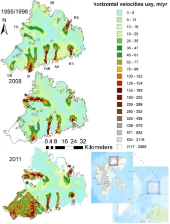
2.2 Remote sensing data of surface velocities

Tandem Phase ERS-1/2 1 day SAR scenes were acquired between December 1995 and January 1996 (1 day interval) and surface ice velocities were calculated using SAR interferometry (InSAR) (henceforth “1995 velocities”, Pohjola et al., 2011; Schäfer et al., 2012). Four ALOS PALSAR scenes were acquired between January 2008 and

5

March 2008 with 46 days time interval and velocities calculated using offset-tracking (henceforth “2008 velocities”, Pohjola et al., 2011). For 2011, an ERS-2 SAR data stack acquired in March/April with a 3 days time interval processed with a combined InSAR and tracking approach similar to the 1995 data (Pohjola et al., 2011) is used (referred as “2011 velocities”, unpublished data). In all cases the vertical components of the

10

velocities have been neglected during the calculation of horizontal velocities.

The velocity error in the InSAR data is 2 cm, which corresponds to 7 m yr−1for Tan-dem ERS-1/2 SAR data (1 day time interval) and 2 m yr−1 for 3-days ERS-2 SAR data (Dowdeswell et al., 2008). By considering a matching error estimate of 1/10th of a pixel, the precision of offset-tracking is about 10 m yr−1for the 2008 ALOS PALSAR data

sep-15

arated by a temporal interval of 46 days (Pohjola et al., 2011). In the 2011 ERS-2 data set, dual-azimuth o_ffset-tracking was considered in the northern part of Vestfonna and here the matching error is estimated to be about 35 m yr−1; in the southern part SAR data of only one orbit is available and the error of range-azimuth offset tracking is larger, on the order of 130 m yr−1.

20

The 2008 and 2011 data sets do not cover the ice cap completely, and data gaps have been filled by interpolation and smoothing, except for the south-western corner (a region of slow flow), where the 1995 data were used to fill a larger data gap (ne-glecting possible variations in Gimlebreen).

The surface velocities are presented in Fig. 1 (before interpolation and patching). We

25

(8)

TCD

7, 5097–5145, 2013

M. Schäfer et al.

Title Page

Tables Figures

◭ ◮

Back Close

Full Screen / Esc

Discussion

P

a

per

|

D

iscussion

P

a

per

|

Discussion

P

a

per

|

Discuss

ion

P

a

per

large changes occurred, though on Franklinbreen the southern branch continued to ac-celerate slightly, while the northern branch deac-celerated. The speed up of Franklinbreen, the flow feature showing the biggest change since 1995 (reaching speeds comparable to other fast flowing outlet glaciers in 2008/2011), is modest compared to other Sval-bard surging glaciers (Hagen et al., 1993).

5

2.3 Thermal boundary conditions

Di_fferent thermal boundary conditions are required in the model, one being surface or air temperature. Svalbard’s climate has a maritime character with cooler summers and warmer winters than is typical at such a high latitude (Möller et al., 2011). Mean monthly air temperatures on VSF still do not exceed₊3 ◦C, and winter monthly means

10

fall between−10 ◦C and−15 ◦C with minimum values of the order of−25◦C to−40 ◦C (Möller et al., 2011). A lapse rate approach is used in the current study to prescribe the surface temperatures

T_surf(x)₌T_sea(x)−γS(x) (1)

at the surface elevationS(x). We use a lapse rateγ=0.004 K m−1(Wadham and

Nut-15

tall, 2002; Wadham et al., 2006; Schuler et al., 2007a). This value is close to the one adopted in other studies:γ=0.0044 K m−1(Pohjola et al., 2002); Liljequist (1993) found a slightly larger lapse rate ofγ=0.005 K m−1from measurements between the summit of Vestfonna (known as Ahlmann summit) and the 1957/58 IGY station at Kinnvika. Comparison with data from the atmospheric model WRF (Skamarock et al., 2008;

20

Hines et al., 2011) during 1989–2010 confirms this approach, since a mean lapse rate of 0.0042 K m−1with variations up to 30 % corresponding to up to 1 K in the different di-rections (B. Claremar Uppsala, personal communication, 2013) is found. We estimate the mean air temperature at sea level,T_sea(x), with the same lapse rate approach from data collected during 2005 to 2009 at various weather stations on Austfonna and

Vest-25

(9)

TCD

7, 5097–5145, 2013

M. Schäfer et al.

Title Page

Tables Figures

◭ ◮

Back Close

Full Screen / Esc

Discussion

P

a

per

|

D

iscussion

P

a

per

|

Discussion

P

a

per

|

Discuss

ion

P

a

per

In addition, the geothermal heat flux is an important basal boundary condition. Con-trary to Schäfer et al. (2012) who assumed a geothermal heat flux of 63 mW m−2 typi-cal for post-Precambrian, non-orogenic tectonic regions (Lee, 1970), we take the value of 40 mW m−2, which is motivated by the measured gradients of profiles obtained by deep drilling on the Nordaustlandet ice caps (Zagorodnov et al., 1989; Ignatieva and

5

Macheret, 1991; Motoyama et al., 2008). In the case of Nordaustlandet, ground sur-face temperature changes in the uppermost 1–2 km of the bedrock are most likely still influenced by the cold of the Weichselian period, explaining this lower measured value of 40 mW m−2and leading to good simulations of an observed (via deep drilling) tem-perature profile on VSF (Motoyama et al., 2008), as explained in Sect. 4.2.

10

3 Model description

Here only the most relevant equations of the model are presented. The dynamics of the forward model are described in Sect. 3.1 (and further details including some parameter values in the Appendix A). The heat transfer equation and the di_fferent heat sources are detailed in Sect. 3.2. In Sect. 3.3 the inverse method applied to infer the basal

15

friction coefficientβis summarized. Finally in Sect. 3.4 the mesh is presented.

The model equations are solved numerically with the Elmer/Ice model. It is based on the open-source multi-physics package Elmer developed at the CSC – IT Center for Science in Espoo, Finland, and uses the finite-element method (Zwinger et al., 2007; Gagliardini and Zwinger, 2008; Gagliardini et al., 2013).

20

3.1 Forward model

(10)

TCD

7, 5097–5145, 2013

M. Schäfer et al.

Title Page

Tables Figures

◭ ◮

Back Close

Full Screen / Esc

Discussion

P

a

per

|

D

iscussion

P

a

per

|

Discussion

P

a

per

|

Discuss

ion

P

a

per

the strain rates ˙ǫthrough Glen’s law, which in index notation reads

˙

ǫ_ij =A(T)τ_⋆2τ_ij′. (2)

The temperature dependency of the deformation rate factor,A(T), is described by an Arrhenius law

A(T)₌A₀exp(−Q/[R(273.15₊T)]), (3)

5

whereRis the universal gas constant,A₀the prefactor andQthe activation energy.A₀ andQare given by

A₀=3.985×10−13Pa−3s−1, Q=−60 K J mol−1, T ≤ −10◦C, (4) A₀=1.916×103 Pa−3s−1, Q=−139 K J mol−1, T >−10◦C (Paterson, 1994)

10

The evolution of free surfaceSis governed by the kinematic boundary condition

∂z

∂t +vx

∂z

∂x +vy

∂z

∂y =vz+aonS, (5)

wherearepresents the climate mass balance andvx,y,z the velocity components.Sis assumed to be a stress-free surface, i.e.τ·n=0.

At the lower boundaryB, a linear friction law (Weertman type law, Robin type

bound-15

ary condition Greve and Blatter, 2009) is imposed

t·(τ·n)₊β(x,y)v·t=0, onB, leading tov_||= 1

β(x,y)τ||, (6)

wherenandtare normal and tangential unit vectors,βis the basal friction parameter and v_|| and τ_|| are the basal velocity and stress components parallel to the bed. We assume zero basal melting (v·n=0). The basal friction coefficient field β(x,y) will be

20

(11)

TCD

7, 5097–5145, 2013

M. Schäfer et al.

Title Page

Tables Figures

◭ ◮

Back Close

Full Screen / Esc

Discussion

P

a

per

|

D

iscussion

P

a

per

|

Discussion

P

a

per

|

Discuss

ion

P

a

per

On the lateral boundaries the normal stress is set to the water pressure exerted by the oceanp_w

(

p_w=−ρ_wgz, ifz<0m,

p_w=0, otherwise, (7)

wherez is elevation a.s.l., g gravitational acceleration and ρ_w=1025 kg m−3 is sea-water-density.

5

3.2 Temperature model

Schäfer et al. (2012) use a temporally fixed depth dependent temperature profile (here referred to as depth dependent temperature profile)

T(x)₌T_surf(x)₊qgeo

κ D(x), (8)

whereq_geo=40 mW m−2is the geothermal heatflux,κ=2.072 W K−1m−1a mean heat

10

conductivity andD(x) the ice depth (distance to the surface at a given locationxin the ice body). In contrast, the current study uses the heat transfer equation to evolve the ice temperature distribution, which reads (expressed in terms of temperature,T)

ρc _∂

T

∂t +v· ∇T

=∇.(κ∇T)+QwithT ≤T_pm, (9)

whereT_pmis the pressure melting point (Zwinger et al., 2007),ρis the ice density and

15

Qa volumetric heat source. The heat capacityc and heat conductivityκare functions of temperature, turning Eq. (9) into a non-linear problem:

c(T)=146.3+7.253T (unit J kg−1K−1), (10)

(12)

TCD

7, 5097–5145, 2013

M. Schäfer et al.

Title Page

Tables Figures

◭ ◮

Back Close

Full Screen / Esc

Discussion

P

a

per

|

D

iscussion

P

a

per

|

Discussion

P

a

per

|

Discuss

ion

P

a

per

At the upper boundary a Dirichlet condition is imposed onT using the parametrization described in Sect. 2.3. At the bed a heat flux is imposed composed of geothermal heat flux,q_geo=κgradT·n, and friction heat qf =ubτb (withub the sliding velocity and τb the basal drag).

The volumetric heat source Q comprises strain heat Q_s=2µǫ⋆, where ǫ⋆ is the

5

second invariant of the strain rate tensor, and latent heat from firn heating Q_l (latent heat released during refreezing of percolating melt water). Q_l is calculated using the P_max model of Wright et al. (2007) as used by Zwinger and Moore (2009). Different characteristic shapes of the time averaged temperature-depth profilesT(d) in summer and winter are used (Wright et al., 2007):

10

T(d)=

d d_ice−1

(Ta−Tw)+Ta, in the winter, (12)

T(d)=Ta 1−

(d−d_ice)2

d_ice2 !1₂

, in the summer, (13)

whered is the depth below the surface. There are three free parameters in this firn heating parametrization:T_aandT_ware the annual and winter mean air temperatures

15

respectively set according to Sect. 2.3.d_ice is the typical penetration depth of the an-nual temperature cycle which is kept as a free parameter and tuned to reproduce the measurements in the deep ice core (Motoyama et al., 2008), see Sect. 4.2.

The resulting volume heat source is deduced by the di_fference of internal energy defined by the difference∆T(d) between the seasonal profiles Eqs. (12) and (13)

20

Q_l(d)₌cρ∆T(d), (14)

(13)

TCD

7, 5097–5145, 2013

M. Schäfer et al.

Title Page

Tables Figures

◭ ◮

Back Close

Full Screen / Esc

Discussion

P

a

per

|

D

iscussion

P

a

per

|

Discussion

P

a

per

|

Discuss

ion

P

a

per

3.3 Inverse model

A variational inverse method (Arthern and Gudmundsson, 2010) is used in this study to infer the spatially varying basal friction coefficientβ(x,y). It is based on the minimiza-tion of a cost funcminimiza-tion when solving the Stokes Equaminimiza-tions iteratively with two di_fferent sets of boundary conditions. The definition of the cost function and the minimization

5

algorithm follow Gillet-Chaulet et al. (2012) and Jay-Allemand et al. (2011). This ap-proach is similar to Schäfer et al. (2012) but with the addition of a regularization term (Habermann et al., 2012).

The method iteratively applies a Neumann and a Dirichlet condition at the upper free surface. In the Dirichlet problem the Neumann free upper surface condition is replaced

10

by a Dirichlet condition where the observed surface horizontal velocities are imposed

v_hor(x)₌v_obs(x),∀x∈S, (15)

wherev_hor(x) andv_obs(x) stand respectively for the modeled and observed horizontal surface velocities. Inz-direction, (τ·n)·e_z₌0 is imposed on S, where e_z is the unit vector along the vertical. To avoid unphysical negative values, the friction parameter

15

fieldβ(x,y) is expressed asβ=10α and the minimization of the cost function is per-formed with respect toα. The cost function, which expresses the mismatch between the two solutions for the velocity field with di_fferent boundary conditions on the upper surfaceS, is given by

J₀(β)=

Z

S

(vN−vD)·(τN−τD)·ndA, (16)

20

(14)

TCD

7, 5097–5145, 2013

M. Schäfer et al.

Title Page

Tables Figures

◭ ◮

Back Close

Full Screen / Esc

Discussion

P

a

per

|

D

iscussion

P

a

per

|

Discussion

P

a

per

|

Discuss

ion

P

a

per

the first spatial derivatives ofα is added to the total cost functionJ_tot

J_tot=J₀+λJ_reg, (17)

J_reg=1

2 Z

B _∂α

∂x 2

+

_∂α

∂y 2

dA, (18)

whereλis a positive parameter (see Sect. 4.1.1 for its choice). The minimization of the

5

cost function is thus a compromise between best fit to observations and smoothness ofα, determined by the tuning ofλ. The minimization algorithm is described by Gillet-Chaulet et al. (2012) and Gagliardini et al. (2013).

3.4 Meshing

Anisotropic mesh refinement is now increasingly used in numerical modeling especially

10

with the finite elements method since the mesh resolution is a critical factor. Schäfer et al. (2012) have investigated effects of varying the resolution in the context of this in-verse method. Here we use again the mesh established with the fully automatic, adap-tive, isotropic surface remeshing procedure Yams (Frey, 2001). A 2-D footprint-mesh was established according to the glacier outline on the 1990 NPI-map and adapted

15

using the metric based on the Hessian matrix of the observed 1995 surface veloc-ities. Horizontal resolution varies between 250 m and 2500 m. Finally the mesh was extruded vertically in 10 equidistant terrain following layers according to the bedrock and surface data. In the simulations involving firn heating, the mesh was extruded ver-tically in 20 layers with the upper 10 layer thicknesses reducing towards the surface

20

(15)

TCD

7, 5097–5145, 2013

M. Schäfer et al.

Title Page

Tables Figures

◭ ◮

Back Close

Full Screen / Esc

Discussion

P

a

per

|

D

iscussion

P

a

per

|

Discussion

P

a

per

|

Discuss

ion

P

a

per

4 Simulations

In this section we present the setup of our simulations. In Sect. 4.1 the unfeasibility of an ideal thermo-mechanical spin-up is addressed and we describe our alternative tem-perature initialization. In the distribution of the basal sliding coe_fficient regulating the velocity field is determined before a purely mechanical spin-up is conducted (surface

5

relaxation, Sect. 4.1.2). These simulations are thereafter the starting point for simula-tions to investigate and validate the influence of the different heat sources, especially to calibrate our firn heating parametrization (Sect. 4.2). A short prognostic simulation is also conducted (Sect. 4.3), emulating the observed acceleration of Franklinbreen with different scenarios with the goal to link the corresponding changes in the basal drag

10

coe_fficient to variations in temperature or other factors.

4.1 System initialization

The inherent problem if starting from a DEM purely on observed data, is that an in-stantaneous solution for both the mechanical and the thermo-dynamical problems is needed as a starting point. Thermal initial conditions are critical in modeling of

poly-15

thermal glaciers or ice sheets because of the energy storage capacity of ice, the low advection/diffusion rates on the glacier and the strong thermo-mechanical coupling via the ice viscosity. An ideal spin-up would demand a transient run starting from deglaciated conditions with a long enough spin-up time requiring realistic forcing (tem-perature, mass balance) as well as knowledge of the velocity field. That’s because the

20

VSF temperature distribution at any given instant in time is a function of past evolution of the advection, diffusion of heat and heat sources – friction heating being a major heat source and having a strong time dependency for glaciers with time variable veloc-ities. Air temperature and precipitation records exist over a long enough time. However a precise reconstruction of the velocity field of VSF will not be feasible until we can

25

(16)

TCD

7, 5097–5145, 2013

M. Schäfer et al.

Title Page

Tables Figures

◭ ◮

Back Close

Full Screen / Esc

Discussion

P

a

per

|

D

iscussion

P

a

per

|

Discussion

P

a

per

|

Discuss

ion

P

a

per

In the absence of such ideal spup we assume steady-state for temperature, in-cluding the e_ffects of strain heating and friction heating, even though non-steady-state conditions have occurred on VSF between 1995 and 2008, and probably on longer time scales as well. We found characteristic timescales to reach such a steady-state to be of the order of several hundreds of years (not shown in this paper). This will lead

5

to over- or underestimations of the temperature depending on the past state of each outlet glacier. In practice the errors will be largest closest to the bed where friction heat production has greatest e_ffect and will decay away in the interior regions of the ice cap. Seroussi et al. (2013) also addressed the question of thermal initial conditions and came to the conclusion that steady-state temperatures based on present-day

con-10

ditions are a reasonable good approximation both for calculations of basal conditions and century-scale transient simulations.

Remaining uncertainties in the model initial conditions (including uncertainties in the model parameters as well as the domain geometry), lead to ice flux divergence anoma-lies (Zwinger and Moore, 2009; Seroussi et al., 2011), resulting in a non-smooth vertical

15

velocity field. Because of the importance of the vertical velocity field for advection of cold ice from the surface, and to smooth out these ice flux divergence anomalies the free surface is relaxed before conducting further transient simulations.

4.1.1 Inverse simulations to derive spatial patterns of the basal friction

The method of Schäfer et al. (2012) is followed with some improvements: correct

ma-20

rine boundary conditions (Eq. 7) are applied, a regularization term in the cost function is added and a better minimization algorithm is used. The simulations to determine the best weight for the regularization term,λ, in Eq. (17) are performed for simplicity with temperature kept fixed to the depth dependent profile (Sect. 3.2) as done by Schäfer et al. (2012). This is justified because of the small temperature dependency as it was

25

(17)

TCD

7, 5097–5145, 2013

M. Schäfer et al.

Title Page

Tables Figures

◭ ◮

Back Close

Full Screen / Esc

Discussion

P

a

per

|

D

iscussion

P

a

per

|

Discussion

P

a

per

|

Discuss

ion

P

a

per

a function of J₀ (match to observations) using the 1995 velocity data. We find J₀ is minimized by settingλ=105.0, which also leads to acceptable smoothness inβ.

In a similar way, we conduct inversions for the basal drag with the 2008 and 2011 surface velocity fields (Fig. 2). These runs are conducted also with the 1990 surface DEM, since no complete additional surface DEM is available. Nuth et al. (2010) and

5

Moholdt et al. (2010) have shown from ICESat laser altimetry data that mean elevation changes over VSF were 0.05 m yr−1 and −0.16 m yr−1 over the periods 1990 to 2005 and 2003 to 2008 respectively. The changes form a complex spatial pattern on VSF, with local values up to 1 m yr−1 in the south. It has been shown (Schäfer et al., 2012) that surface variations of this order (or higher) between 1995 and 2008 or 2011 do not

10

significantly a_ffect the drag fields derived from the inverse method. The same value for theλparameter as well as the same inhomogeneous mesh have been used, the latter to facilitate comparison. The inferred basal drag coefficient distributions clearly reflect the acceleration of Franklinbreen with decreasing values of the friction coe_fficient β

from 1995 to 2008. For the other outlets the general patterns remain similar for the

15

three periods and show only small local variations.

An iteration scheme between inversion and temperature calculation has been tested. The depth dependent temperature profile (Eq. 8) was used in the first inversion for

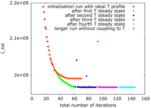
β, then steady-state calculations of the temperature field (accounting for friction and strain heating) and inversions were run alternately. The resultingβdistribution reveals

20

small changes compared to keeping the temperature fixed to the depth dependent pro-file, showing a certain robustness ofβtowards changes in temperature. Nevertheless, the value of the cost function has been decreased with the iterative scheme (Fig. 3), showing an improved match between observed and computed surface velocities. Con-vergence of this iteration was assessed through the cost function and stopped once

25

the cost function stabilized. Convergence of the steady-state temperature field was ascertained through visual inspection.

(18)

simula-TCD

7, 5097–5145, 2013

M. Schäfer et al.

Title Page

Tables Figures

◭ ◮

Back Close

Full Screen / Esc

Discussion

P

a

per

|

D

iscussion

P

a

per

|

Discussion

P

a

per

|

Discuss

ion

P

a

per

tions require high resolution in the vertical), and because of the greater uncertainties associated with this heat source compared to the others. It causes very little change to

β. For further simulations, the distribution ofβ obtained with the iteration scheme but neglecting firn heating is adopted (Fig. 2).

4.1.2 Surface relaxation

5

As initial conditions for transient simulations the free surface is relaxed for three years under zero mass-balance. This relaxation simulation was initialized with output from the inversion-temperature iterations. A short time step (0.1 yr) was chosen to guaran-tee temporal resolution of artificially strong surface changes induced by the remaining uncertainties. Visual inspection of the smoothness and magnitude of the vertical

veloc-10

ity field was used to determine the end of the relaxation procedure.

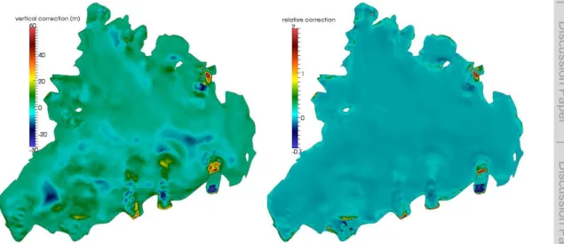
The largest changes to the mesh (Fig. 4) occur in the southwestern corner and in some outlet glaciers where there is a significant paucity of bedrock radar data (see Pettersson et al., 2011, for radar coverage). In these outlet glaciers it is even unknown whether additional mountain ridges or valleys exist at the bedrock underlying fast flow

15

features, or whether such features are only driven by surface topography. Some other less important changes are visible in northeastern VSF – again in areas with sparsely covered bedrock data.

A more complex spin-up scheme involving an iteration between surface relaxation, inverse method and temperature calculation was also tested for a single combination

20

of surface velocity data and included heat sources in the temperature calculation. This procedure requires huge computational e_fforts and does not lead to visible improve-ments in the results (β field, temperature field, and surface corrections) and is hence not used in this work for several di_fferent combinations of surface velocity data (3 pos-sibilities) and included heat sources (6 pospos-sibilities).

25

(19)

TCD

7, 5097–5145, 2013

M. Schäfer et al.

Title Page

Tables Figures

◭ ◮

Back Close

Full Screen / Esc

Discussion

P

a

per

|

D

iscussion

P

a

per

|

Discussion

P

a

per

|

Discuss

ion

P

a

per

4.2 Influence of different heat sources on the temperature distribution

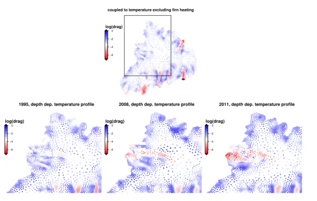
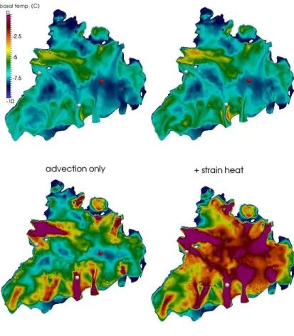
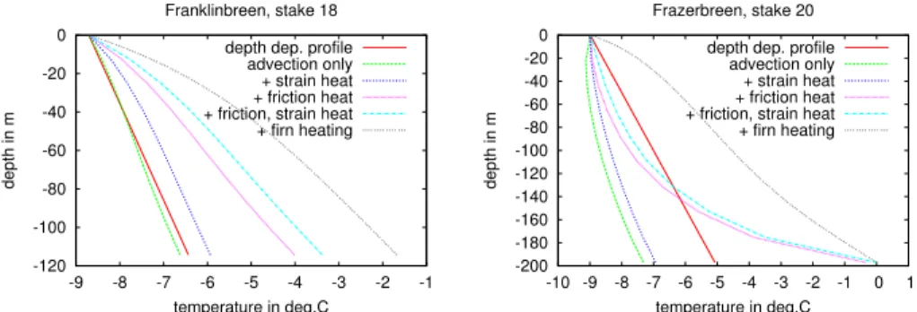
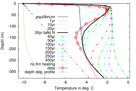
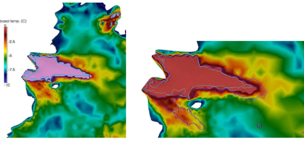
From the model state described above, the influence of the di_fferent heat sources (Sect. 3.2) on the thermal regime of the ice cap are discussed. Results are compared to the temperature profile measured in a drill hole located in the central area of the ice cap at the east end of the summit ridge; see Fig. 5 for the exact location (Motoyama

5

et al., 2008). Figure 6 shows simulated temperature-depth profiles for the various com-binations of heat sources at two other locations on Franklinbreen and Frazerbreen, in the ablation and in accumulation areas respectively. Simulated basal temperatures are shown in Fig. 5.

At the location of the drill hole, using only strain and friction heating, the measured

10

temperature profile cannot be reproduced, even close to the bedrock where these heat sources are most effective, Fig. 7 (brown line compared to the data in red). Various sim-ulations with different parameter sets (free parameterd_ice, temperature parameters) in our firn heating parametrization have been conducted and two qualitative observations could be made: (1) with constant surface forcing only (close to) equilibrium temperature

15

simulations including firn heating do affect the temperature in vicinity of the bedrock; (2) these quasi equilibrium solutions do not feature the clear inflexion in the tempera-ture profile visible close to the surface in the observed data. Such simulations lead to temperature profiles similar to the blue curve in Fig. 7, the profiles are only shifted to warmer or colder temperatures. The green, cyan and pink curves in the figure illustrate

20

the evolution of the temperature profile during a transient simulation and how the inflex-ion of the temperature profile is slowly smoothed out and propagated down towards the bedrock when approaching equilibrium. We thus hypothesize that the observed bore-hole profile results from a succession of two different surface boundary conditions: (1) a low surface temperature and low firn heating over a period long enough to approach

25

(20)

TCD

7, 5097–5145, 2013

M. Schäfer et al.

Title Page

Tables Figures

◭ ◮

Back Close

Full Screen / Esc

Discussion

P

a

per

|

D

iscussion

P

a

per

|

Discussion

P

a

per

|

Discuss

ion

P

a

per

we make the hypothesis that boundary condition changes can be represented in our firn heating parametrization by the penetration depth parameter.

This can be motivated by the fact that ice cores elsewhere in Svalbard indicate that firn heating and percolation have been frequent in the last 500–1000 yr (Van de Wal et al., 2002; Divine et al., 2011). The proportion of ice lenses which indicate periods

5

of near zero ice surface temperatures increased from 33 % during the Little Ice Age to 55 % in the 20 th century, Pohjola et al. (2002). The surface temperatures have been kept fixed to the observations of the weather stations as stated earlier.

We assume that the penetration depth increases linearly from 0 m at the elevation of an average firn line to a maximum penetration depth at the summit, leading to the

10

effect that firn heating increases with the thickness of the firn layer. This is also in line with the usual approach of calculating refreezing as a fraction of winter accumulation, which is best described on VSF by an elevation gradient (Möller et al., 2011). This is a simplification since in reality the melting should be largest at low (warmer) elevation even though the firn thickness increases with altitude, an e_ffect which is at least partially

15

counterbalanced by the formation of ice lenses, more e_ffectively with more melt, which inhibits penetration of melt water.

The mean elevation of the firn line was digitized from several satellite pictures: Land-sat July 1976, September 1988 and August 2006; Spot July 1991 and August 2008; Aster August 2000 and July 2005. Two of these lines (August 2008 and

Septem-20

ber 1988) have been excluded since the firn lines are located at exceptionally low elevations probably due to abnormally early fresh snow. We observe little change over recent decades, as found by Möller et al. (2013). Since the firn line elevation is ap-proximately uniform over most of the ice cap, a single mean elevation for the firn line is assumed ignoring any other spatial variations. We estimate this mean elevation to be

25

(21)

sur-TCD

7, 5097–5145, 2013

M. Schäfer et al.

Title Page

Tables Figures

◭ ◮

Back Close

Full Screen / Esc

Discussion

P

a

per

|

D

iscussion

P

a

per

|

Discussion

P

a

per

|

Discuss

ion

P

a

per

face mass balance the firn line elevation could be parametrized by the elevation of the equilibrium line.

A first run of the model to equilibrium temperature using a maximum penetration depth of 13.5 m leads to a good match with the measurements in the lower part of the drilling hole, see Fig. 7 (blue line). A prognostic run over 30 yr with an increased

5

penetration depth of 18 m starting from this equilibrium state allows then to reproduce fairly well the observed peak in the upper layers (black line). The horizontal distribution of the modeled temperature including firn heating is shown in Fig. 5 and the vertical in Fig. 6.

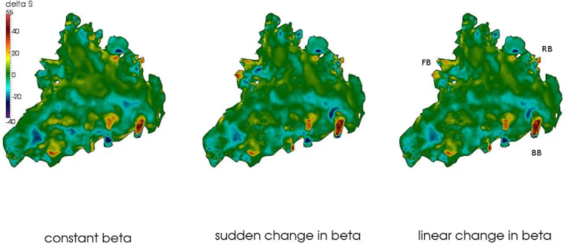
4.3 Prognostic simulations over the period 1995–2008

10

To study the evolution of the temperature field we conduct prognostic simulations with three di_fferent temporal evolutions of β prescribed and analyze the connected evolu-tion of all system variables. The three simulaevolu-tions are run with full thermomechanical coupling starting from the relaxed 1990 DEM, using present day surface mass balance (Möller et al., 2011) as a forcing. Temperature is initialized to the 1995 steady-state

15

temperature profile. The three basal drag scenarios are:

1. The basal drag coefficient kept constant at the 1995 pattern.

2. A sudden switch after five years to the 2008 pattern (which di_ffers from the 1995 pattern mainly by the acceleration of Franklinbreen).

3. A locally linear change from the 1995 to 2008 values.

20

(22)

TCD

7, 5097–5145, 2013

M. Schäfer et al.

Title Page

Tables Figures

◭ ◮

Back Close

Full Screen / Esc

Discussion

P

a

per

|

D

iscussion

P

a

per

|

Discussion

P

a

per

|

Discuss

ion

P

a

per

5 Discussion

5.1 Implications of inferred basal drag coefficient distributions

The basal drag coe_fficientβis a crucial parameter in simulating the thermodynamical regime of VSF as it is a key control on sliding velocities, which govern both friction heat-ing and heat advection. As shown in Sect. 4.1.1, use of an inverse method to derive

5

the spatially varying basal drag coe_fficient is largely una_ffected by temperature distribu-tion. Conversely, the temperature evolution shows high sensitivity to such an inversion. Surface relaxation (Sect. 4.1.2) reduces this sensitivity by producing smoother velocity fields.

Variations in the basal drag coe_fficient distribution across the three periods (Fig. 2)

10

connected to large variations in surface velocities and indicate the importance of a time evolving basal drag based on the underlying physical processes. When comparing the obtained basal patterns from 1995, 2008 and 2011, the internal structure of some of the outlet glaciers is slightly different, but the most striking change remains the acceler-ation of Franklinbreen from 1995 to 2008 featured by a strong increase in basal sliding.

15

The 2011β-distribution mainly reflects the di_fferent changes in velocity pattern in the two branches of Franklinbreen: the northern one is decelerating while the southern one continues to accelerate. Minor changes in the two most eastern outlet glaciers between 2008 and 2011 are more likely artifacts of the data imperfections in the 2008 and 2011 velocity data sets than features of the real system. In all outlet glaciers a distinct

spa-20

(23)

TCD

7, 5097–5145, 2013

M. Schäfer et al.

Title Page

Tables Figures

◭ ◮

Back Close

Full Screen / Esc

Discussion

P

a

per

|

D

iscussion

P

a

per

|

Discussion

P

a

per

|

Discuss

ion

P

a

per

5.2 Interpretation of a temperature profile from deep drilling

As shown in our simulations in which firn heating is represented (Sect. 4.2), the ob-served shape of the temperature profile measured in the Motoyama et al. (2008) ice core (Fig. 7) cannot be explained by an equilibrium temperature profile. Our model-supported interpretation requires a recent perturbation away from an earlier equilibrium

5

state, caused by a change in the surface conditions. Van de Wal et al. (2002) came to a similar conclusion when reconstructing the temperature record in the Lomonosov-fonna plateau (northeast of Billefjorden/Isfjorden, Spitzbergen). However, they kept the surface temperature as tuning parameter. Their obtained surface temperature is too high and induces a shift of a few Kelvin. Hence model and data fit well in the lower part,

10

but the surface values are unrealistically warm. They conclude a change in surface con-ditions in the 1920ies from their model and find confirmation for this by comparing to the mean air temperature record at Svalbard airport starting in 1910.

Discrepancy between our model-implied change in the 60 s and the actual climatic record can be explained by various reasons: first, as stated earlier, the uncertainty in

15

the basal drag coefficient strongly impacts the evolution of the temperature distribution through advection. Second, only one data set of deep borehole temperatures is avail-able for model calibration. Lastly, our approach might be too simplistic, especially with respect to the assumptions of spatial or elevation dependencies, and the use of pen-etration depth as the only calibration parameter (surface temperature variations also

20

lead to temperature variations at depth but with different timescales to the penetration depth).

The calibrated penetration depth (13.5 m and 18 m, Sect. 4.2) is deeper than might be expected, since measured relative densities (Motoyama et al., 2008) reach values over 0.85 at 10 m depth and below, i.e. values of ice or ice lenses with very slow

per-25

(24)

TCD

7, 5097–5145, 2013

M. Schäfer et al.

Title Page

Tables Figures

◭ ◮

Back Close

Full Screen / Esc

Discussion

P

a

per

|

D

iscussion

P

a

per

|

Discussion

P

a

per

|

Discuss

ion

P

a

per

2007), and imply that our approach should be considered as qualitative rather than quantitative.

With respect to this more recent change in the conditions on the surface, our model predicts that this signal will take over 100 yr to reach the base. Thus for studying basal processes, even for prognostic simulations on a century scale, we can neglect the

ef-5

fects of this change in firn heating (see also Fig. 7). Conversion of the latent energy released at the location of the ice core corresponds at the location of the drilling hole to aP_maxvalue of 0.9, which is in the expected range (Wright, 2005), increasing confi-dence in our model.

A discrepancy between our equilibrium profile and the data is also apparent in the

10

middle of the depth profile. We explain this either by the fact that the ice cap has not yet reached thermal equilibrium (see the 50/100/150 yr etc. graphs in Fig. 7 for the shape of such profiles in the lower and middle part) or by the impacts of uncertainties in advection (Sect. 5.1).

With our simplified parametrization of latent heat release due to refreezing we are

15

qualitatively able to reproduce the observed profile, indicating that we identified the driving mechanisms behind the measured distribution. Di_fferent limitations of this model for a better interpretation of quantitative results have been highlighted. However, in view of the relative robustness to temperature variations of the inverse method (Schäfer et al., 2012) we are confident that the remaining uncertainties or imperfections of our

20

approach are justified in terms of the inversion for the basal drag coe_fficient and results with respect to the respective roles of the different heat sources.

5.3 The role of heat sources for VSF fast flowing outlet glaciers

A comparison between surface and sliding velocities at the bedrock clearly shows that sliding dominates the ice dynamics at the fast flow areas of VSF, which even holds for

25

(25)

TCD

7, 5097–5145, 2013

M. Schäfer et al.

Title Page

Tables Figures

◭ ◮

Back Close

Full Screen / Esc

Discussion

P

a

per

|

D

iscussion

P

a

per

|

Discussion

P

a

per

|

Discuss

ion

P

a

per

method. Therefore we focus on the impact of temperature and the respective heat sources on the onset and maintenance of fast flow.

5.3.1 Friction and strain heating

Our results regarding the importance of friction heating are similar to those of Brinker-hoffet al. (2011) for some Greenland outlet glaciers. In the fast outlet glaciers, where

5

basal sliding is important, friction heating is a dominant heat source and is needed to maintain temperate conditions at the bed (Fig. 5). In contrast to Pohjola and Hed-fors (2003), who investigated fast flow in Antarctica using a one-dimensional numerical thermodynamic model, the contribution of strain heating is found to be very small on VSF. Strain heat integrated over the whole ice column is at least an order of magnitude

10

lower than friction heat at the bed. Strain heat is mainly confined to the shear margins while friction heat is present over the whole bedrock area of the outlet glaciers. Larour et al. (2012) observed a similar spatial distribution of strain and friction heat, however they find similar magnitudes for both heat sources.

The pattern of simulated friction heating is consistent with the fast flow and sliding

ar-15

eas, except for some of the southern facing outlet glaciers which appear in our results to be cold-based yet fast flowing. Brinkerhoffet al. (2011) discussed the possibility of cold based sliding or underestimation of ice deformation due to neglecting ice anisotropy. Here, cold based sliding occurs mainly in areas where the bedrock elevation is poorly known, so that uncertainties in the ice thickness are certainly the main factor to explain

20

why basal ice does not reach the pressure melting point. Irregularities in the bedrock data and analysis of the 1995–2008 prognostic simulations (Sect. 5.4) confirm this; improvement of the bedrock data by some control method should be considered as for example done by Morlighem et al. (2013) or van Pelt et al. (2013).

Even though this clear correlation between friction heat and sliding was identified,

25

(26)

TCD

7, 5097–5145, 2013

M. Schäfer et al.

Title Page

Tables Figures

◭ ◮

Back Close

Full Screen / Esc

Discussion

P

a

per

|

D

iscussion

P

a

per

|

Discussion

P

a

per

|

Discuss

ion

P

a

per

outlet glaciers and the only outlet glacier featuring some areas with sub-melt sliding (Hindmarsh and Meur, 2001), even in the absence of additional heat sources. By its reduced ice velocities it might have thickened enough to allow basal ice to approach pressure melting point through insulation and in turn triggering sliding. Thickening of Franklinbreen especially in the lower part between 1990 and 2005 is confirmed by Nuth

5

et al. (2010). Various temperature feedbacks like the one involving friction heating could then have reinforced and maintained this acceleration. However, no complete surface DEMs from di_fferent periods are available. Neither Nuth et al. (2010) nor Moholdt et al. (2010) observed a thinning on Franklinbreen between 1990–2005 or between 2003– 2008. Even though Nuth et al. (2010) observe large errors over Franklinbreen (average

10

0.06±0.12 myr−1) it seems unlikely that the recent reduction of the acceleration visible from comparing the 2008 and similar 2011 velocities on Franklinbreen is driven simply by a negative feedback involving thinning.

5.3.2 Firn heating due to melt water refreezing

Firn heating is important for the general thermal regime of the ice cap and can have

15

larger impacts than friction or strain heating in some regions (Figs. 5 and 6). Our model shows an increase in basal temperature in the onset area of Franklinbreen due to firn heating (Fig. 5). However, since similar increases occur at non-accelerating glaciers, we rule this out as the sole trigger for speed-ups of outlet glaciers. It would still have an impact on the basal sliding of already fast flowing glaciers. The temperature signal

20

of a recent increase in latent heat release cannot possibly have reached the bedrock to explain the recent acceleration (Fig. 7). Also because of the long di_ffusive time scale (centuries) for temperature (Fig. 7) we do not expect firn heating to be the maintaining mechanism behind a lasting acceleration. Nevertheless it could be possible that firn heating has indirect impacts a_ffecting the englacial hydrology.

(27)

TCD

7, 5097–5145, 2013

M. Schäfer et al.

Title Page

Tables Figures

◭ ◮

Back Close

Full Screen / Esc

Discussion

P

a

per

|

D

iscussion

P

a

per

|

Discussion

P

a

per

|

Discuss

ion

P

a

per

5.4 Evolution of the temperature field in prognostic runs

Focusing on Franklinbreen, as expected in scenario (1) (see Sect. 4.3) the velocity pat-tern remains constant. In scenario (2) a sudden increase in velocities after the change in basal drag coe_fficient is followed by a small deceleration. In scenario (3) the velocities increase synchronous with changes in basal drag coe_fficient (Fig. 2). The 2008

veloci-5

ties are identical in scenarios (2) and (3). Scenarios (2) and (3) exhibit a clear thinning of the onset area of Franklinbreen relative to (1) (Fig. 8). This is more pronounced (up to 25 m compared to 20 m) in scenario (2) resulting from the time integrated ice flux which is higher the sooner the velocities increase. The pronounced increase in thick-ness at the terminus of Franklinbreen can be interpreted as a model feature caused

10

by fixing geometry horizontally and neglecting calving. Other outlet glaciers, especially Rijpbreen and Bodlebreen, are highly influenced by errors in the bedrock DEM and thus not discussed.

Temperature remains unchanged in scenario (1). In scenarios (2) and (3) however, the model shows a warming of around 2 K at Franklinbreen’s lateral margins.

Tempera-15

ture changes are not restricted to ice at the bed. An approach to designing a physically based sliding law would be to allow sliding where temperature approaches pressure melting point. The area in which this occurs increases slightly in both scenarios. In scenario (2), the temperature adjusts smoothly during the years following the jump to a similar pattern as in scenario (3); no sudden jump in basal temperature is visible in

20

spite of the step change in basal drag coefficient. The friction heat production changes in the same way in scenarios (2) and (3) over Franklinbreen and its onset area, reach-ing fairly high up to the center of the ice cap. Similarly strain heat increases in both scenarios at the lateral margins of Franklinbreen and over the whole ice column. In scenario (2), both heat sources undergo a sudden jump synchronous with the jump

25

(28)

TCD

7, 5097–5145, 2013

M. Schäfer et al.

Title Page

Tables Figures

◭ ◮

Back Close

Full Screen / Esc

Discussion

P

a

per

|

D

iscussion

P

a

per

|

Discussion

P

a

per

|

Discuss

ion

P

a

per

high, but the fine structure of the basal drag coefficient distribution is not closely related to that of friction heat.

In scenario (2) all velocities and heat sources adjust instantly to the step change in basal drag coefficient whereas the temperature field lags a few time steps behind. However, the final temperatures of scenarios (2) and (3) are very close which allows

5

for an estimation of basal temperature adjustment to take place in the order of years to decades. Taking into account a few years for adjustment we see good agreement for all variables after this 13 yr period with scenarios (2) and (3), suggesting that the simulations are robust towards the detail of how changes in basal drag coefficient occur. When comparing the steady-state temperature field obtained with the 1995 basal

10

drag coe_fficient (henceforth 1995ss), the steady-state temperature field obtained using the 2008 basal drag coefficient (2008ss) and the final temperature distribution of the 1995–2008 prognostic simulation with linear changing basal drag coefficient (scenario 3), two main observations can be made: firstly, the result of the 1995–2008 prognostic simulation and 2008ss show di_fferences mainly in the central, slow flowing areas. This

15

implies that in these areas at least one of the steady-state assumptions is wrong, since the timescale to reach steady-state is too long. Secondly, when comparing the changes during the prognostic simulation and the di_fference between 1995ss and 2008ss, they are rather similar around Franklinbreen. This means that in the areas of fast flow, or even changing fast flow, temperature seems to reach steady-state fairly quickly and

20

our steady-state assumption is justified. Note that the 2008ss distribution has been calculated in two different ways, either by using a relaxation with the 2008 infered basal drag pattern, or by using the relaxation with the 1995 pattern and recalculating the new velocity field before calculating temperatures. Both approaches are identical except for small areas on the southern and northern margins.

25