ISSN 0104-6632 Printed in Brazil
www.abeq.org.br/bjche
Vol. 31, No. 01, pp. 109 - 117, January - March, 2014
Brazilian Journal
of Chemical
Engineering
MIXED CONVECTION FLOW BY A POROUS SHEET
WITH VARIABLE THERMAL CONDUCTIVITY
AND CONVECTIVE BOUNDARY CONDITION
T. Hayat
1,2, S. A. Shehzad
1*, M. Qasim
3and A. Alsaedi
21Department of Mathematics, Quaid-i-Azam University 45320, Islamabad 44000, Pakistan. *
E-mail: [email protected] 2
Department of Mathematics, Faculty of Science, King Abdulaziz University, P.O. Box 80257, Jeddah 21589, Saudi Arabia.
3
Department of Mathematics, Comsats Institute of Information Technology, Park Road, Chak Shehzad, Islamabad 44000, Pakistan.
(Submitted: June 7, 2012 ; Revised: November 8, 2012 ; Accepted: December 4, 2012)
Abstract - Effects of variable thermal conductivity on the mixed convection flow over a porous stretching surface are investigated. Analysis has been performed subject to the convective boundary conditions. The fluid is electrically conducting in the presence of a uniform applied magnetic field. The resulting problems are computed. The effects of emerging parameters on the velocity and temperature profiles are displayed and discussed. The values of the skin-friction coefficient and local Nusselt number are analyzed numerically.
Keywords: MHD flow; Variable thermal conductivity; Convective boundary condition.
INTRODUCTION
Stretching flow is an important topic of research undergoing rapid growth amongst the recent investi-gators. Such interest of researchers is due to the broad range of practical applications of such flows in engineering, including extrusion processes, glass fi-bers and paper production, drawing of plastic films, crystal growing and many others. Stretched flows have been extensively analyzed since the seminal work of Sakiadis (1961) in view of diverse aspects including heat and mass transfer, MHD, suction/in-jection, non-Newtonian fluids, similar and non-simi-lar solutions etc. For example, Kechil and Hashim (2009) addressed the MHD stagnation point flow of viscous fluid in a porous medium. The Adomian decomposition method was utilized for the expres-sions of velocity and temperature. Thermal radiation effects in unsteady magnetohydrodynamic (MHD) flow have been discussed by Hayat and Qasim (2010). Here the series solutions are computed by the
110 T. Hayat, S. A. Shehzad, M. Qasim and A. Alsaedi
were performed without considering the convective boundary conditions. Few authors take into account such boundary conditions. For example, Aziz (2009) analyzed the impact of convective type boundary conditions on the boundary layer flow of a viscous fluid over a flat plate. Yao et al. (2011) investigated the heat transfer analysis in a viscous fluid over a stretching/shrinking sheet with convective boundary conditions. Ishak (2011) also studied the flow problem with convective boundary conditions. All these studies have been restricted to the situations of constant thermal conductivity. Chiam (1998) exam-ined the effects of variable thermal conductivity on the boundary layer flow of a viscous fluid over a stretching sheet. Chiam (1996) also discussed the stagnation point flow of a viscous fluid towards a stretching sheet in the presence of variable thermal conductivity. Sharma and Singh (2008) investigated the viscous flow and heat transfer with variable ther-mal conductivity.
However, no attempt has yet been presented for the effect of variable thermal conductivity on the flow due to a stretched sheet with convective bound-ary conditions. Such a concept is important in the sense that thermal conductivity for liquid metals varies with temperature in a linear manner in the range of 00F to 4000F (Vyas and Rai, 2010). Hence, the aim of the present study is to investigate the MHD mixed convection flow over a stretching sur-face with convective boundary conditions when the thermal conductivity of the fluid is variable. The homotopy analysis method (HAM) was applied to find the series solutions of the problem (Liao, 2003, 2004; Abbasbandy and Shivanian, 2010, 2011; Hashim et al., 2009; Hayat et al., 2010, 2011, 2012). The solutions developed are displayed and discussed.
PROBLEM STATEMENT
Here we choose the Cartesian coordinate system in such a manner that the x−axis is along the stretched sheet and the y−axis is normal to it. We consider the MHD mixed convection flow of a vis-cous fluid with convective boundary conditions over a porous stretching sheet. All the physical properties of the fluid except the thermal conductivity are taken to be constant. The thermal conductivity varies linearly with the temperature. Neglecting the radia-tive and viscous dissipation effects, the boundary layer equations are:
0, ∂ +∂ = ∂ ∂ u v (1) 2 2 0 2 ( ∞) ,
∂ + ∂ = ν∂ + β − −σ
∂ ∂ ∂ T ρ
u u u B
u v g T T u
x y y (2)
,
⎛ ∂ ∂ ⎞ ∂ ⎛ ∂ ⎞
ρ ⎜ + ⎟= ⎜ ⎟
∂ ∂ ∂ ∂
⎝ ⎠ ⎝ ⎠
p
T T T
C u v k
x y y y (3)
with the boundary conditions:
( ) , ,
( ) at 0,
= = = ∂ − = − = ∂ w w f
u u x cx v v
T
k h T T y
y
(4)
0, ∞ as .
→ → → ∞
u T T y (5)
Note that the temperature boundary condition in Eq. (4) indicates that the bottom surface of the sheet is heated by convection from a hot fluid at temperature Tf , providing a heat transfer coefficient
.
h In the above equations u and v are the velocity components parallel to the x− and y−axes respec-tively, ν the kinematic viscosity, βT the thermal ex-pansion coefficient, T the temperature, k the vari-able thermal conductivity, ρ the density of the fluid,
p
C the specific heat at constant pressure and c the rate of stretching. The magnetic Reynolds number is chosen small and thus the induced magnetic field is neglected.
We introduce the following variables (Yao et al., 2011):
( ), ( ), ,
( ) f
c
u cxf c f y
T T
T T
∞ ∞ ′
= η ν = − ν η η =
ν −
θ η = −
(6)
where c is a constant, prime denotes the differentiation with respect to η and we consider Tw( )x =
( )
T∞+Dxα∗θ η at η =0 and variable thermal con-ductivity k=k∞[1+ εθ], k∞ is the fluid free stream conductivity and ε is defined as:
( )
. ∞ ∞ − ε = kw k
k (7)
Mixed Convection Flow with Variable Thermal Conductivity and Convective Boundary Condition 111
2 2
0, ′
′′′+ ′′− + λθ − ′=
f ff f M f (8)
2
(1+ εθ θ + εθ =) ′′ ′ Pr[α θ − θ∗ f′ f ′], (9) , / , (1 (0))
at 0,
′ ′
= = = α θ = −γ − θ
η =
f S f b c
(10)
0, 0 as , ′ = θ = η → ∞
f (11)
in which 1/2
Re λ = x
x Gr
where Grx= βg T( f −T∞)x3/ν2 is the local Grashoff number and Rex =u xw /ν is the local Reynolds number, 2 σ 02
ρ = B
c
M is the Hartman number, γ =hk νc is the Biot number and Pr Cpk
∞
ρ ν = is the Prandtl number.
The skin-friction coefficient Cf and local Nusselt number Nux are defined as
2 , ( ),
/ 2 w w f x f w xq C Nu
k T T
U ∞
τ
= =
−
ρ (12)
in which τw and qw are given by:
0 0
, .
= =
⎛∂ ⎞ ⎛∂ ⎞
τ = μ⎜ ⎟ = − ⎜ ⎟
∂ ∂ ⎝ ⎠ ⎝ ⎠ w w y y u T q k
y y (13)
On a dimensionless scale, Eq. (12) becomes:
1/2 1/2
1
Re (0), / Re (0).
2Cf x = f′′ Nu x = −θ′ (14)
SOLUTIONS EMPLOYING HAM
We express f and θ in the set of base functions: {ηkexp(− η ≥n )k 0,n≥0}, (15)
as follows
0
0,0 , 0 0
( ) exp( ),
∞ ∞
= =
η = +
∑∑
k ηk − ηm n n k
f a a n (16)
, 0 0
( ) exp( ),
∞ ∞
= =
θ η =
∑∑
k ηk − η m nn k
b n (17)
in which am nk, and bm nk, are the coefficients.
The initial approximations and auxiliary linear operators are given below:
0( )η = −1 exp(−η), θ η =0( ) exp(−η),
f (18)
, θ ,
′′′ ′ ′′
= − = θ − θ
f
L f f L (19)
with:
1 2 3
4 5
( ) 0,
( ) 0,
f
L C C e C e
L C e C e
η −η
η −η
θ
+ + =
+ =
(20)
where Ci(i= −1 5) denote the arbitrary constants. The following problems corresponding to the zeroth order deformations are constructed:
(
1)
ˆ( ; ) 0( )ˆ( ; ), ( ; ) ,ˆ f
f f
q L f q f
p f q q
⎡ ⎤
− ⎣ η − η =⎦
⎡ η θ η ⎤
⎣ ⎦
= N
(21)
(
1)
ˆ( ; ) 0( )ˆ( ; ), ( , ) ,ˆ
q L q
p f q q
θ
θ θ
⎡ ⎤
− ⎣θ η − θ η⎦
⎡ ⎤
= = N ⎣ η θ η ⎦
(22)
ˆ(0; ) , (0; )ˆ 1, ( ; )ˆ 0, ˆ(0; ) (1 (0; ), ( , )ˆ 0,
′ ′
′ ′
= = ∞ =
θ = −γ − θ θ ∞ =
f q S f q f q
q q q
(23)
2
3 2
2
3 2
ˆ( , ) ˆ( , ) ˆ( , ) ˆ( , )
ˆ ˆ
[ ( , )] ( , ) ( , ) ,
f
f q f q f q f q
f ηq =∂ η +f ηq ∂ η −⎜⎜⎛∂ η ⎞⎟⎟ + λθ ηq −M ∂ η
∂η ∂η
∂η ∂η ⎝ ⎠
N (24)
2
2 2
2 2
ˆ( , ) ˆ( , ) ˆ( , ) ˆ( , ) ˆ( , )
ˆ ˆ ˆ ˆ ˆ
[ ( , ), ( , )]q f q q ( , )q q q Pr ∗ ( , )q f q Pr ( , )f q q , θ
⎛ ⎞
∂ θ η ∂ θ η ∂θ η ∂ η ∂θ η
θ η η = + εθ η + ε⎜⎜ ⎟⎟ − α θ η + η
∂η ∂η ∂η
∂η ∂η ⎝ ⎠
112 T. Hayat, S. A. Shehzad, M. Qasim and A. Alsaedi
where q∈[0,1] is an embedding parameter, =f and θ
= are the non-zero auxiliary parameters and Nf and Nθ the nonlinear operators. Note that for q=0 and 1q= we have:
0 0
ˆ( ;0) ( ), ( ,0)ˆ ( )
ˆ ˆ
and ( ;1) ( ), ( ,1) ( ),
η = η θ η = θ η
η = η θ η = θ η
f f
f f
(26)
and as q increases from 0 to 1 then ( , )f ηq and ( , )
θ ηq vary from f0( ),η θ η0( ) to ( )f η and ( ).θ η Expanding f and θ in Taylor's series we obtain:
0
1
( , ) ( ) ( ) , ∞
=
η = η + ∑ η m
m m
f q f f q (27)
0
1
( , ) ( ) m( ) m, m
q q
∞
=
θ η = θ η + ∑ θ η (28)
0
0
1 ( ; )
( ) ,
!
1 ( ; )
( ) , ! = = ∂ η η = ∂η
∂ θ η θ η =
∂η m m m q m m m q f q f m q m
(29)
where the convergence of the above series strongly depends upon =f and =θ. Assuming that =f and
θ
= are selected properly so that (21) and (22) con-verge at q=1, then:
0
1
( ) ( ) ( ), ∞
= η = η + ∑ m η
m
f f f (30)
0
1
( ) ( ) ( ).
∞
= θ η = θ η + ∑ θ ηm
m
(31)
The problems at m th-order are:
1
[ ( )η − χ − ( )]η = Rm( ),η
f m m m f f
L f f h (32)
1
[ ( ) ( )] ( ),
θ θ η − χ θm m m− η = θ θRm η
L h (33)
(0) (0) ( ) 0, (0) (0) ( ) 0,
m m m
m m m
f f′ f′
′
= = ∞ =
θ − γθ = θ ∞ =
(34)
1
1 1 1
0 2 1 1 ( ) ( ) ( ) ( ), m m
f m m k k m k k
k
m m
f f f f f
M f − ′′ ′′′ ′′ ′ ′ − − − − − = ′ − − ⎡ ⎤
η = η + ∑ ⎣ − ⎦
+λθ η − η
R
(35)
1 1
1 1 1
0 0
1 1
1 1
0 0
( )
Pr Pr ,
m m
m
m m k k m k k
k k
m m
m k k m k k
k k
f f
− −
′′ ′′ ′ ′
θ − − − − −
= =
− −
∗ ′ ′
− − − −
= =
η = θ + ε ∑ θ θ + ε ∑ θ θ
− α ∑ θ + ∑ θ
R
(36)
The general solutions are:
1 2 3
( )η = ∗( )η + + η+ −η,
m m
f f C C e C e (37)
4 5
( ) ∗( ) η −η,
θ η = θ η +m m C e +C e (38)
where fm∗ and θ∗m are our special solutions.
CONVERGENCE ANALYSIS
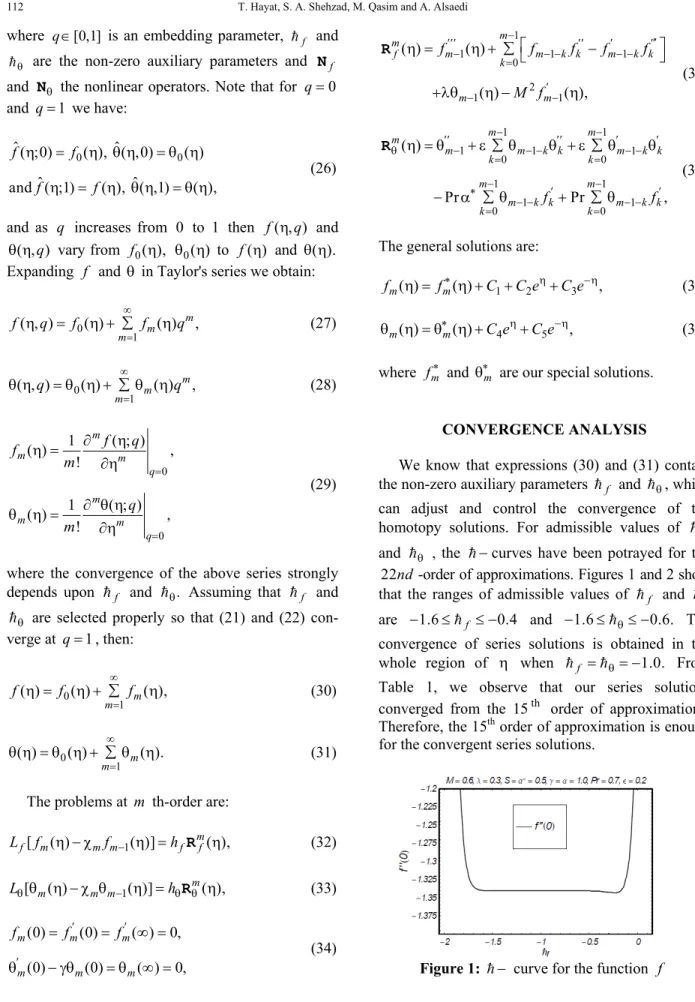
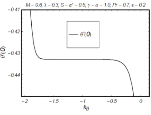
We know that expressions (30) and (31) contain the non-zero auxiliary parameters =f and =θ, which can adjust and control the convergence of the homotopy solutions. For admissible values of =f and =θ , the =−curves have been potrayed for the
22nd-order of approximations. Figures 1 and 2 show that the ranges of admissible values of =f and =θ are −1.6≤=f ≤ −0.4 and −1.6≤=θ≤ −0.6. The convergence of series solutions is obtained in the whole region of η when =f ==θ= −1.0. From Table 1, we observe that our series solutions converged from the 15th order of approximations. Therefore, the 15th order of approximation is enough for the convergent series solutions.
Mixed Convection Flow with Variable Thermal Conductivity and Convective Boundary Condition 113
Figure 2: =− curve for the function θ
Table 1: Convergence of homotopy solutions for different orders of approximations when M= 0.6,
0.3,
λ = S= α =∗ 0.5, γ = α =1.0, Pr=0.7, ε =0.2
and =f ==θ= −1.0.
Order of approximation -f′′(0) -θ′(0)
1 1.35500 0.46042
5 1.34241 0.43457
10 1.34043 0.43293
15 1.34035 0.43286
20 1.34035 0.43286
30 1.34035 0.43286
40 1.34035 0.43286
DISCUSSION
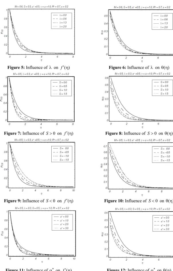
The effects of emerging parameters on velocity and temperature are shown in this section. Hence Figures 3 20− are plotted for various values of the Hartman number M, buoyancy parameter ,λ suction/ injection parameter S, positive constant α∗, Biot number ,γ Prandtl number Pr and small parameter ε on velocity and temperature profiles f′ η( ) and
( )
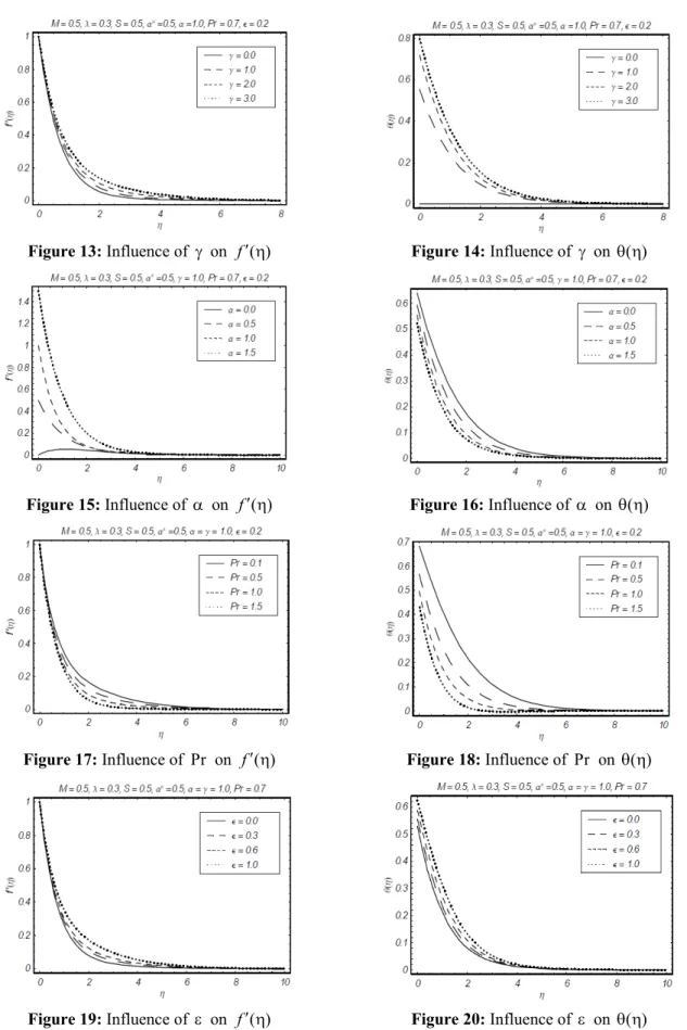
θ η , respectively. Figures 3 and 4 indicate the velocity ( )f′ η and temperature ( )θ η for the Hartman number M. Figure 3 shows that an increase in Hartman number M decreases the fluid velocity and boundary layer thickness. This trend for the thermal boundary layer is quite opposite (see Figure 4) . It is evident from Figure 5 that the velocity f′ η( ) in-creases as the parameter λ increases, while the thermal boundary layer decreases (Figure 6 ). It is observed from Figures 7 and 8 that both the velocity and temperature profiles decrease with an increase in suction parameter S>0. However, the opposite trend is observed for the injection parameter S<0 (see Figures 9 and 10 ). Figure 11 shows that the velocity field decreases upon increasing the parame-ter α∗. Figure 12 shows that α∗ exerts a similar role on temperature and velocity in a qualitative sense. We can see from Figures 13 and 14 that, by increasing
,
γ both the velocity and temperature fields increase. By comparing Figures 15 and 16, we conclude that α gives the opposite results for f′ η( ) and ( ).θ η Figures 17 and 18 describe the influence of Pr on
( )
′ η
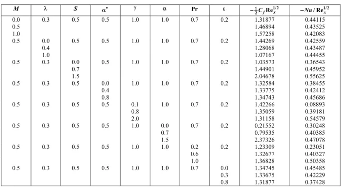
f and ( ).θ η Upon increasing Pr, both velocity and temperature decrease. The parameter γ has simi-lar effects on velocity and temperature profiles (see Figures 19 and 20). Table 2 is constructed for the numerical values of the skin-friction coefficient and local Nusselt number. This table shows that, by increasing M, the values of the skin-friction coeffi-cient increase, whereas the local Nusselt number decreases. However, increasing ,λ we observed op-posite results. An increase in S and λ∗ causes an increase in both the skin-friction coefficient and the local Nusselt number.
114 T. Hayat, S. A. Shehzad, M. Qasim and A. Alsaedi
Figure 5: Influence of λ on f′ η( ) Figure 6: Influence of λ on ( )θ η
Figure 7: Influence of S>0 on f′ η( ) Figure 8: Influence of S>0 on ( )θ η
Figure 9: Influence of S<0 on f′ η( ) Figure 10: Influence of S<0 on ( )θ η
Mixed Convection Flow with Variable Thermal Conductivity and Convective Boundary Condition 115
Figure 13: Influence of γ on f′ η( ) Figure 14: Influence of γ on ( )θ η
Figure 15: Influence of α on f′ η( ) Figure 16: Influence of α on θ η( )
Figure 17: Influence of Pr on f′ η( ) Figure 18: Influence of Pr on ( )θ η
116 T. Hayat, S. A. Shehzad, M. Qasim and A. Alsaedi
Table 2:Values of the skin-friction coefficient 1 1/2 x
2C Ref and the local Nusselt number
1/2
/ Re
−Nu x for different values of M, ,λ ,S α∗, γ, ,α Pr and .ε
M λ S α∗ γ α Pr ε 1 1/2
2 Re
− Cf x −Nu/ Re1/2x
0.0 0.3 0.5 0.5 1.0 1.0 0.7 0.2 1.31877 0.44115
0.5 1.46894 0.43525
1.0 1.57258 0.42083
0.5 0.0 0.5 0.5 1.0 1.0 0.7 0.2 1.44269 0.42559
0.4 1.28068 0.43487
1.0 1.07167 0.44455
0.5 0.3 0.0 0.5 1.0 1.0 0.7 0.2 1.03573 0.36543
0.7 1.44901 0.45952
1.5 2.04678 0.55625
0.5 0.3 0.5 0.0 1.0 1.0 0.7 0.2 1.32584 0.38455
0.4 1.33775 0.42412
0.8 1.34743 0.45686
0.5 0.3 0.5 0.5 0.1 1.0 0.7 0.2 1.42266 0.08893
0.8 1.35059 0.39181
2.0 1.31158 0.54579
0.5 0.3 0.5 0.5 1.0 0.0 0.7 0.2 0.21552 0.30248
0.7 0.79535 0.40385
1.5 2.37326 0.47078
0.5 0.3 0.5 0.5 1.0 1.0 0.2 0.2 1.23309 0.23051
0.6 1.32677 0.40327
1.0 1.36828 0.50358
0.5 0.3 0.5 0.5 1.0 1.0 0.7 0.0 1.34745 0.45485
0.3 1.33675 0.42229
0.8 1.31877 0.37428
CLOSING REMARKS
Mixed convection flow of a viscous fluid with variable thermal conductivity and convective boundary conditions is discussed. The main results are sum-med up as follows:
The velocity field f′ η( ) decreases upon increas-ing M and the temperature field ( )θ η increases when
M increases.
Both ( )f′ η and ( )θ η increase when γ is in-creased.
An increase in Pr leads to a decrease in the velocity and temperature profiles.
The thermal boundary layer thickness decreases upon increasing Pr .
α∗ has similar effects on f′ η( ) and ( )θ η in a qualitative sense.
ACKNOWLEDGMENT
We are grateful to the reviewer for his/her valuable suggestions. The first and second author are grateful to the Higher Education Commission of Pakistan (HEC) for the financial support. The re-search of Dr. Alsaedi was partially supported by
the Deanship of Scientific Research (DSR), King Abdulaziz University, Saudi Arabia.
REFERENCES
Abbasbandy, S. and Shivanian, E., Prediction of multiplicity of solutions of nonlinear boundary value problems: Novel application of homotopy analysis method. Commun. Nonlinear Sci. Numer. Simulat., 15, p. 3830 (2010).
Abbasbandy, S. and Shivanian, E., Predictor homotopy analysis method and its application to some nonlin-ear problems. Commun. Nonlinnonlin-ear Sci. Numer. Simulat., 16, p. 2456 (2011).
Aziz, A., A similarity solution for laminar thermal boundary layer over a flat plate with a convective surface boundary condition. Commun. Nonlinear Sci. Numer. Simulat., 14, p. 1064 (2009).
Bhattacharyya, K. and Layek, G. C., Effects of suction/blowing on steady boundary layer stagna-tion-point flow and heat transfer towards a shrinking sheet with thermal radiation. Int. J. Heat Mass Transfer, 54, p. 302 (2011).
Mixed Convection Flow with Variable Thermal Conductivity and Convective Boundary Condition 117
Chiam, T. C., Heat transfer with variable conduc-tivity in a stagnation-point flow towards a stretch-ing sheet. Int. Commun. Heat Mass Transfer, 32, p. 239 (1996).
Fang, T., Zhang, J. and Yao, S., Slip MHD viscous flow over a stretching sheet-An exact solution. Commun. Nonlinear Sci. Numer. Simulat., 14, p. 3731 (2009).
Hashim, I., Abdulaziz, O. and Momani, S., Homo-topy analysis method for fractional IVPs. Commun. Nonlinear Sci. Numer. Simulat., 14, p. 674 (2009).
Hayat, T. and Qasim, M., Effects of thermal radia-tion on unsteady magnetohydrodynamic flow of a micropolar fluid with heat and mass transfer. Z Naturforsch A., 64, p. 950 (2010).
Hayat, T. and Qasim, M., Influence of thermal radiation and Joule heating on MHD flow of a Maxwell fluid in the presence of thermophoresis. Int. J. Heat Mass Transfer, 53, p. 4780 (2010). Hayat, T., Qasim, M. and Abbas, Z., Radiation and
mass transfer effects on the magnetohydrody-namic unsteady flow induced by a stretching sheet. Z Naturforsch A. 64, p. 231 (2010).
Hayat, T., Shehzad, S. A., Qasim, M. and Obaidat, S., Radiative flow of Jeffery fluid in a porous medium with power law heat flux and heat source. Nuclear Eng. Design, 243, p. 15 (2012). Hayat, T., Shehzad, S. A., Qasim, M. and Obaidat,
S., Thermal radiation effects on the mixed con-vection stagnation-point flow in a Jeffery fluid. Z Naturforsch A. 66, p. 606 (2011).
Ishak, A., Thermal boundary layer flow over a stretching sheet in a micropolar fluid with radia-tion effect. Meccanica, 45, p. 367 (2010).
Ishak, A., Yacob, N. A. and Bachok, N., Radiation effects on the thermal boundary layer flow over a moving plate with convective boundary condi-tion. Meccanica, 46, p. 795 (2011).
Kechil, S. A. and Hashim, I., Approximate analytical solution for MHD stagnation-point flow in porous media. Commun. Nonlinear Sci. Numer. Simulat., 14, p. 1346 (2009).
Liao, S. J., Beyond Perturbation: Introduction to Homotopy Analysis Method. Chapman and Hall, CRC Press, Boca Raton (2003).
Liao, S. J., On the homotopy analysis method for nonlinear problems. Appl. Math. Comput., 147, p. 499 (2004).
Sakiadis, B. C., Boundary-layer behavior on continu-ous solid surface: I. Boundary-layer equations for two-dimensional and axisymmetric flow. AIChE J., 7, p. 26 (1961).
Salleh, M. Z., Nazar, R. and Pop, I., Boundary layer flow and heat transfer over a stretching sheet with Newtonian heating. J. Taiwan Institute Chem. Engin., 41, p. 651 (2010).
Sharma, P. R. and Singh, G., Effects of variable thermal conductivity and heat source/sink on MHD flow near a stagnation point on a linearly stretching sheet. J. Appl. Fluid Mech., 2, p. 15 (2008).
Tsai, R. and Huang, J. S., Numerical study of Soret and Dufour effects on heat and mass transfer from natural convection flow over a vertical porous medium with variable wall heat fluxes. Comput. Materials Sci., 47, p. 23 (2009).
Vyas, P. and Rai, A., Radiative flow with variable thermal conductivity over a non-isothermal stretch-ing sheet in a porous medium. Int. J. Contemp. Math. Sciences, 5, p. 2685 (2010).
Yao, B. and Chen, J., Series solution to the Falkner-Skan equation with stretching boundary. Applied Math. Comput., 208, p. 156 (2009).