L’emploi rural et urbain au Brésil: une démarche de données dynamique
Padrones de empleo rural y urbano en Brasil: un enfoque en datos del panel dinámico
Evanio Mascarenhas Paulo1 Francisco José Silva Tabosa2
Recebido em 16/12/2017; revisado e aprovado em 05/05/2018; aceito em 23/05/2018 DOI: h p://dx.doi.org/10.20435/inter.v19i4.1791
Abstract: This study applies a quan ta ve approach in dynamic panel data to capture the determinants of
employment quality in Brazil through the model of generalized minimum moments. The results show that
the rural universe persists as a more precarious environment than urban areas, although the diff erences
has decreased with me. In addi on, the results of this study show that growth of labor income and the level of educa on of employees are important tools not only to expand the levels of job quality, but also as response to dilemmas of the surveyed labor markets.
Keywords: labor market; occupa on quality; panel data; agricultural and non-agricultural employment.
Resumo: Este estudo aplica uma abordagem quan ta va de dados em painel dinâmico por meio sistema
de mínimos momentos generalizados para captar os determinantes da qualidade do emprego no Brasil. Os resultados mostram que o universo rural persiste como um ambiente mais precário que as áreas urbanas, embora essas diferenças tenham diminuído com o tempo. Adicionalmente, os resultados desse estudo mostram que o crescimento da renda do trabalho e do nível de educação dos trabalhadores são fatores importantes para expandir o nível de qualidade do emprego e também como resposta aos dilemas dos mercados de trabalho pesquisados.
Palavras-chave: mercado de trabalho; qualidade das ocupações; emprego agrícola e não agrícola.
Résumé: Dans ce e étude, une approche quan ta ve de données de panel est appliquée pour capturer les
condi ons de qualité de l’emploi à travers le modèle des moments minimum généralisés. Sur les résultats, l’univers rural persiste comme un environnement plus précaire par rapport aux zones urbaines, même si les
diff érences ont diminué au fi l du temps. On a fait valoir que le revenu des travailleurs et le niveau d’éduca on
sont importants pour l’expansion de la qualité de l’emploi, mais aussi une stratégie pour surmonter dilemmes des marchés analysés.
Mots-clés: marche du travail; qualite de l’occupa on; panneau de donnees; emploi agricole et non agricole.
Resumen: En este estudio se aplica un cuan ta vo enfoque en datos de panel para captar condicionantes
de la calidad del empleo en Brasil, a través del modelo de mínimos momentos generalizados. Sobre los resultados, el universo rural persiste como un ambiente más precario cuando se compara con las zonas urbanas, aunque las diferencias hayan disminuido con el empo. La inves gación mostró también que el crecimiento de los ingresos del trabajo y el nivel de escolaridad de los trabajadores son instrumentos importantes para la ampliación de los niveles de calidad del empleo, sino también estrategia de superación de dilemas de los mercados de trabajo analizados.
Palabras clave: mercado laboral; calidad de la ocupación; panel de datos; empleo agrícola y no agrícola.
1 INTRODUCTION
Authors, such as Balsadi (2007), Schneider (2005) e Da Silva (1998), have promoted eff orts to undo the dis nc on between rural and urban areas. These authors argue that current human development needs have not been met by projects aimed to remove this disparity, as shown by Da Silva (1998), These authors use labor market elements to explain these needs, since the
1 Pon cia Universidade Católica do Rio Grande do Sul (PUC-RS), Porto Alegre, Rio Grande do Sul, Brasil.
2 Universidade Federal do Ceará (UFC), Campus Pici, Fortaleza, Ceará, Brasil.
Es
te é um ar
go public
ado em acesso abert
o (Open Access) sob a licenç
a Cr
ea
v
e Commons A
ribu
on, que permit
e
uso
, dis
tribuiç
ão e r
epr
oduç
ão em qualquer meio
, sem r
es
triç
ões desde que o tr
abalho original seja c
labor market mirrors the transforma on that occurs in the rural areas from the introduc on of labor-saving technologies, which aim to reducing costs and increasing produc vity.
Already for Schneider (2005), the behavior of the labor market, which is subject to the logic of produc on rela ons, is infl uenced by the movement of phenomena that aff ect the agricultural paradigm, transla ng into a con nuous increase of labor produc vity in agricultural ac vi es because of the introduc on of innova ve technologies and moderniza on of agriculture.
In this regard, Da Silva (1998) states that, as a func on of changes in produc ve units, two major types of transforma on occur in the agricultural labor market. First, there is a new division of labor within family units, as some members of families are released for work in other ac vi es, beyond the family produc on unit. Second, family members who are involved in ag-ricultural work have reduced work me, in order to enable combining agag-ricultural work for the family with other produc ve ac vi es.
Da Silva (1998) goes further to say that diff erence between these two types of on is unit of analysis ‒ the fi rst relates to families and their members, while the second concerns the agricultural establishment, observing the me devoted to farming ac vi es by people.
In the fi rst case, individuals released by the moderniza on process remain in rural areas, but work in ac vi es that are not necessarily agricultural, thereby expanding and consolida ng this category of residents in rural areas. Therefore, if spa al migra on from the countryside to the city has decreased, as observed in Alves e Paulo (2012, p. 51), then the transfer from the rural labor force to non-agricultural ac vi es describes the sectoral migra on of laborers, which has increased considerably, according to Paulo (2015). He s ll has iden fi ed that the migra on of this type of worker to the non-agricultural labor market in many cases occurs under precarious condi ons, because of the low qualifi ca ons of this worker type.
It is noted that the impacts the quality standards of their occupa ons decrease when compared to their work in agriculture, because the agricultural produc ve structure, before the moderniza on process, had even more precarious working condi ons than non-agricultural sectors. Thus, even though the new occupa ons are precarious, they are s ll be er than the previous ones.
This study aims to analyze the components of the quality of occupa on of rural workers in Brazil, by considering recent aspects of produc on rela ons in rural areas and their implica ons for labor rela ons. In par cular, this study discusses recent changes in the rural labor market, with special emphasis on the impacts caused by transforma on in the rural areas. In addi on, this study checks the quality level of rural occupa ons in Brazil based on a job quality index, in order to iden fy contribu ng factors to the quality of rural occupa ons using a panel data model.
2 CONCEPTUAL AND METHODOLOGICAL ASPECTS
2.1 Dataset and construc on of employment quality index
This research seeks to iden fy the condi ons of the quality of occupa ons for four major popula on groups. The fi rst comprises urban agricultural employees, consis ng of employed, salaried people, both formal and informal, in ventures and agricultural groups domiciled in rural areas. The second group of workers comprises urban non-agricultural wage earners and non-agricultural enterprises domiciled in urban regions. The third group comprises employees engaged in agricultural ac vi es and who live in rural areas. Finally, the fourth group comprises rural non-agricultural enterprise employees.
For Nascimento et al. (2007), the percep on of job quality can vary in several aspects as macroeconomic environment, sector structure, among others. However, the inten on in this research is to consider variables in the labor market relevant to the quality of employment, such as the absence of child labor, the regular weekly journey, register in offi cially registered, the contribu on to social security ins tutes and yield.
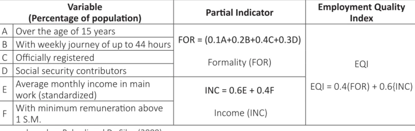
In this way, the Employment Quality Index (EQI), in this study, is an adapta on of the em-ployment quality index formulated ini ally by Balsadi (2007).
Table 1 – Methodology of construc ng employment quality index
Variable
(Percentage of popula on) Par al Indicator
Employment Quality Index
A Over the age of 15 years
FOR = (0.1A+0.2B+0.4C+0.3D)
Formality (FOR) EQI
EQI = 0.4(FOR) + 0.6{INC) B With weekly journey of up to 44 hours
C Offi cially registered
D Social security contributors
E Average monthly income in main work (standardized) INC = 0.6E + 0.4F
Income (INC) F With minimum remunera on above 1 S.M.
Source: based on Balsadi and Da Silva (2008)
Second, following Nascimento et al. (2007), the EQI is used to from the weighted average of par al indicators. According to the authors, the weight of each par al indicator for composi on of the EQI refl ected the rela ve contribu ons. Of the indicators, only average monthly income had to be standardized to a range from 0 to 1. These indicators are used to build two par al indexes from the weighted arithme c averages of the original indicators. Soon, two segments are considered for the calcula on of the index of employment: formality and income. Each of these par al indicators iden fi es elements about the presence or absence of formal work and income levels of workers. The weighted average of the par al indicators demonstrates that a general index, considering the necessary arbitrariness, can help in the analysis of the quality of employment, thereby contribu ng to a more detailed understanding of the condi ons of work.
2.2 Descrip on of variables
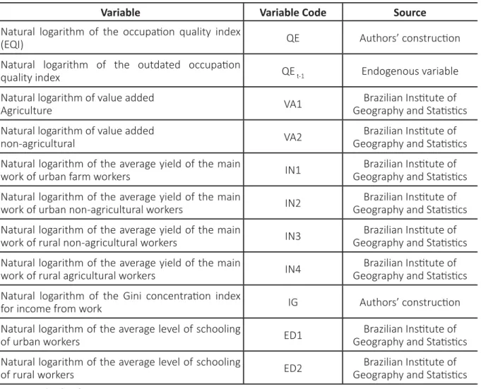
For the iden fi ca on of occupa ons of the groups that this research aims to analyze, this study builds a conglomerate of variables that can synthesize the constraints of the standard quali es of labor rela ons. These variables are summarized in Table 2.
employment contracts and the pa ern of income of workers. Thus, it indicates how sophis cated the working rela onships are. Then, it will be possible to check for possible diff erences between the recruitment of labor in rural areas in agriculture compared to contractual rela ons in urban areas and in ac vi es of non-agricultural segments, so as to trace their determinants and con-tribu ons to employment quality.
The next variable described (QEt–1) is the outdated EQI, which is a feature of the econometric modeling type, selected in this research, to evaluate the proper es of working rela onships. It is expected that this variable is sta s cally signifi cant in that the quality of employment in the previous period is the determinant of the quality of future employment. This hypothesis is due to the natural movement of the dynamics of the labor market, which tends to improve working rela onships over me, being remote the return to a previous pa ern and the presence and specifi c characteris cs of labor laws that secure a contractual rela onship to be pursued by the market and a retrac on of those rights could result in a disregard for labor laws.
Table 2 – Survey variables and code and source of variables
Variable Variable Code Source
Natural logarithm of the occupa on quality index
(EQI) QE Authors’ construc on
Natural logarithm of the outdated occupa on
quality index QE t-1 Endogenous variable
Natural logarithm of value added
Agriculture VA1
Brazilian Ins tute of Geography and Sta s cs
Natural logarithm of value added
non-agricultural VA2
Brazilian Ins tute of Geography and Sta s cs
Natural logarithm of the average yield of the main
work of urban farm workers IN1
Brazilian Ins tute of Geography and Sta s cs Natural logarithm of the average yield of the main
work of urban non-agricultural workers IN2
Brazilian Ins tute of Geography and Sta s cs
Natural logarithm of the average yield of the main
work of rural non-agricultural workers IN3
Brazilian Ins tute of Geography and Sta s cs
Natural logarithm of the average yield of the main
work of rural agricultural workers IN4
Brazilian Ins tute of Geography and Sta s cs
Natural logarithm of the Gini concentra on index
for income from work IG Authors’ construc on
Natural logarithm of the average level of schooling
of urban workers ED1
Brazilian Ins tute of Geography and Sta s cs Natural logarithm of the average level of schooling
of rural workers ED2
Brazilian Ins tute of Geography and Sta s cs
Source: author’s informa on.
the income level of workers and improving working condi ons. Another op on for this variable is that the level of agricultural ac vi es is unrelated to the increase in the quality of the labor market. Thus, economic growth extends to new hires the same contractual rela ons already exis ng, and thus, there are no changes in the structure.
The variable AV2, which expresses the value added of non-agricultural ac vi es, is expected to exert posi ve eff ects on the quality of occupa ons, to the extent that the increase of jobs, which in the case of non-agricultural ac vi es, tends to have greater complexity and higher quality than agricultural occupa ons. Furthermore, just as in the previous case, the variable in ques on might not be related to increased quality of employment contracts, because this does not necessarily mean changes in contrac ng rela onships.
In addi on, search assesses cross-eff ects behavior, that is, the eff ects that economic growth in the non-agricultural ac vi es has on the dynamics of the agricultural and rural employment and economic growth of agricultural ac vi es have on the quality of non-farm employment and urban employment.
The group of variables “IN” expresses the average income level of the main work for each study group evaluated. Thus, the express level IN1 is the average income of urban agricultural workers; IN2 is the average yield of non-agricultural workers; IN3 is the average income of rural non-agricultural workers; and, fi nally, IN4 is the average income of rural farm workers.
It is expected that as the level of real wages increases, it may regress on addi onal real in-come gains, which improves the quality of occupa ons in very informal sectors, due to increased opportunity costs.
The variable “IG” expresses the Gini index, which measures the level of concentra on of income from work. Thus, this variable is evaluated as if it distributes the structure of labor income, that is, how focused the job market is in each State. The expected nega ve sign is jus fi ed by the percep on that the increasing concentra on of income standard tends to decrease the quality of the occupa ons. It is assumed that in the case of this insignifi cant coeffi cient, the quality of work is independent of the concentra on of income in the labor market. Thus, the growth of income guarantees, by itself, the quality of growth occupa ons, even if this means changes in the structure of concentra on.
Finally, the variable “ED” expresses the average educa on level for those who reside in urban areas (ED1) and those who reside in rural areas (ED2). Considering that common sense assumes that the higher the level of educa on, the greater is work effi ciency, and that the general quality of work increases if level of educa on increases.
2.2.1 Method of generalized moments
The nature of various economic rela ons is dynamic and complex, making purely sta c analysis, some mes inadequate or ineffi cient, for understanding the needs of these rela on-ships the work. An advantage of panel data is that they allow understanding the dynamics of adjustment. This dynamic rela onship is characterized by the presence of a lagged dependent variable among the explanatory variables (BALTAGI, 2005). Thus, the following model is used:
The text assume still that ui t follows a one-way error component model, where ui t – (ui + vi t) and ui~IID(0, θu) e vi t~IID(0, θv) are independent of each other and among themselves. “The dynamic panel data regression described in (1) and ui t is characterized by two sources of persistence over me. The autocorrela on is due to the presence of a lagged dependent variable among the regressors and individual eff ects characterizing the heterogeneity among the individuals” Baltagi (2005, p. 135). The a en on that the described model produces are es mators skewed by conven onal es mates. In this perspec ve now, the objec ve on analyz-ing recent econometric models that propose new procedures to es mate and test in the model. Thus, this research proposes an approach conform Baltagi (2005). Therefore, this study employs the system generalized method of moments (system GMM), developed in the works of Arellano and Bond (1991; ), Arellano and Bover (1995), Bond, Hoeffl er and Temple (2001) and Blundell and Bond (1998). In summary, this research uses panel data to es mate models speci-fi ed, in the regression models the following four equa ons:
ln(QEAU) = β0 + β1ln(QEt - 1) + β2ln(VA1) + β3ln(VA2) + β4ln(IN1) + β5ln(IG) + β6ln(ED1) + Vt + μit (2)
ln(QENU) = β0 + β1ln(QEt - 1) + β2ln(AV1) + β3ln(AV2) + β4ln(IN2) + β5ln(IG) + β6ln(ED1) + Vt + μit (3)
ln(QENR) = β0 + β1ln(QEt - 1) + β2ln(AV1) + β3ln(AV2) + β4ln(IN3) + β5ln(IG) + β6ln(ED2) + Vt + μit (4)
ln(QEAR) = β0 + β1ln(QEt - 1) + β2ln(AV1) + β3ln(AV2) + β4ln(IN4) + β5ln(IG) + β6ln(ED2) + Vt + μit (5)
where the dependent variable is the QE of each unit of the federa on and their subscripts refer to agricultural employment (AU), urban non-farm employment (NU), rural non-agricultural (NR), and rural agricultural (AR), respec vely; QEt - 1 expresses the outdated EQI, no ng that in
each case, this variable represents the lagged dependent variable for each group. The on of this variable is characteris c of this type of econometric modeling; AV1 represents the value added in the agricultural ac vi es of each unit of the federa on; AV2 expresses the value added in the non-agricultural ac vi es of each unit of the federa on; IN1 represents the average yield of the main agricultural ac vi es in urban work in the reference week in the fi rst equa on;
IN2 represents the average yield of the main work in urban non-agricultural ac vi es in the reference week in the second equa on; IN3 represents the average yield of the main work in rural non-agricultural ac vi es in the reference week in the third equa on; IN4 represents the average yield of main agricultural rural work in the reference week in the fourth equa on; IG
expresses the level of concentra on of the average yields for each state, measured by the Gini index; ED1 represents the average level of educa on of the urban workers of each subna onal unit in the fi rst two equa ons; ED2 represents the average level of educa on of rural workers at a subna onal unit in the last two equa ons; Vi is the observable eff ects of individuals; and μi t represents the random disturbances. The subscripts i and t refer to the i-th State in year t, respec vely.
..., t, these assump ons being valid for all the other equa ons of the models presented above. The works presented in the literature, in par cular that of Arellano and Bond (1991), high-light some problems in es ma ng these models by tradi onal techniques. The fi rst, problem is due to the presence of the observable eff ects of individuals, Vt along with the lagged dependent variable in period QEt - 1 on the right side of the equa on. In this case, omission of the individual fi xed eff ects panel dynamic model makes the ordinary least squares es mator (MQO) skewed and inconsistent. However, the es mator within groups, which fi xes for presence of fi xed ef-fects, generates an es mated βi skewed downward on panels with small temporal dimension. The second problem is due to the likely endogeneity of explanatory variables. In this case, the endogeneity in the right side of the equa ons must be treated to avoid possible bias generated by a concurrency problem.
Araújo (2009) states that a possible method of trying to overcome this problem would be to eliminate the presence of the fi xed-eff ects model (equa ons presented above). Thus, a fi rst a empt would be to es mate the models through ordinary least squares (MQO) with dummy
variables for each state or through the method within groups, which generates the same es -mates of the previous method, but with standard devia ons of slightly smaller coeffi cients. The coeffi cient es mators for both methods are smaller than the MQO obtained. However, it could be shown that the bias in dynamic panel data con nues to exist.
Nonetheless, according to Araújo (2009), another way to eliminate these problems would be to take the fi rst diff erence of the above equa ons and treat them by the GMM. This method is usually called diff erence GMM and consists of the elimina on of fi xed eff ects through the fi rst diff erence of the previous equa ons. Therefore, equa on (1), for example, was transformed into equa on (6) as follows:
Δln(QEAU) = β0 + β1Δ(lnQEt-1) + β2Δ(lnVA1) + β3Δ(lnVA2) + β4Δ(IN1) + β5Δ(lnIG) + β6Δ(lnED1) + Vt + μit (6)
where for any variable, Yi t, ΔlnYi t = lnYi t - lnYi t - 1. Note that in the above equa ons, ΔlnQEt - 1 is correlated with the error terms, Δlnμi t. Therefore, the ordinary least squares es mator (MQO) for their coeffi cients will be skewed and inconsistent. Therefore, it is necessary to use instrumental variables for ΔlnQEt - 1 and in each model.
The assump ons adopted in the equa ons presented earlier in this sec on imply that the condi ons of moments E
[Δ
lnQEt - 1 Δlnμi t]
= 0 for t = 3, 4, ..., n and s ≥ 2 are valid. Based on these moments, Arellano and Bond (1991) suggest hiring lnQEt - 1 for t = 3, 4, ..., n and s ≥ 2 as instruments for the equa on of fi rst diff erence.The other explanatory variables can be classifi ed as: (a) strictly exogenous, if is not correlated
with the error terms in the past, present and future; (b) weakly exogenous, if is correlated only with values passed the error term and (c) endogenous, if correlated with the error terms in the past, present and future. (ARAÚJO, 2009, p. 61).
In the second case, the lagged variable values in one or more periods are valid instruments in the es ma on equa on and in the la er case, values that are off by two or more periods are valid instruments in es ma ng this equa on.
As Arellano and Bover (1995) and Blundell and Bond (1998) show, these instruments are weak when the dependent and explanatory variables feature strong persistence and/or the
consistent and is skewed to panels with small T.
Therefore, Arellano and Bover (1995) and Blundell and Bond (1998) propose a system that combines the set of equa ons into diff erence equa on (2), with the level equa ons, equa on (1), to reduce this problem of bias. This system is called the system GMM. For the diff erence equa ons, the set of instruments is the same as described above. For regression in level, the appropriate instruments are lagged diff erences of their variables. For example, assume that the diff erences of the explanatory variables are not correlated with the individual fi xed eff ects (for t = 3, 4, ..., n) E
[Δ
lnQEt - 1 μi t] = 0 for i = 1, 2, ..., n. Then, the explanatory variables in diff er-ences and ΔlnQEt - 1 if they are exogenous or weakly exogenous are valid instruments for the equa ons. The same is true if these variables are endogenous, but with the instruments being explanatory variables in a period, lagged diff erences and ΔlnQEt - 1 are considered in this study (ARAÚJO, 2009).System GMM estimates the results from the method of standard error correction (WINDMEIJER, 2005) to prevent underes ma ng the true variance in a fi nite sample. The es -mator used is proposed by Arellano and Bond (1991) in two steps. In the fi rst step, it is assumed that the error terms are independent and homoscedas c in the states and over me. In the second stage, the residues obtained in the fi rst step are used to build a consistent es mate of variance–covariance, relaxing the assump ons of independence and scapular. The second-stage es mator is asympto cally more effi cient in rela on to the fi rst-stage es mator (ARAÚJO, 2009).
Finally, as a way to test the robustness and consistency of the model, Arellano and Bond (1991) suggest two types of tests. The Sargan test is used to verify the validity of the instruments. Failure to reject the null hypothesis indicates that the instruments are robust. Furthermore, since it is assumed that the itε error is not autocorrelated, a fi rst-order serial correla on test and a second-order correla on test are performed on the fi rst-diff erence residues Δ⎕
i t. It is expected
that these errors will be correlated in the fi rst order and not autocorrelated in the second order (ARAÚJO, 2009).
3 EMPLOYMENT QUALITY INDEX: EMPIRICAL RESULTS
This sec on presents and discusses the results of the econometric model presented in Subsec on 2.2, rela ng the EQI for the four groups surveyed to some variables that synthesize the constraints of the structure of the labor market. Therefore, this sec on is organized by the interpreta on of the following Tables 3–6 concerning es mates of the four proposed equa ons. The interpreta on begins with data on urban and agricultural employment, followed by urban and non-agricultural employment, rural non-agricultural employment and fi nally agricultural rural employment.
Table 3 – Ordinary least squares es mates, fi xed eff ects, and generalized least squares for the urban agricultural labor market
Variables
Ordinary least squares [A]
Fixed-eff ects model [B]
Generalized least squares [C]
Coef. Stat. (t) p-value Coef. Stat. (t) p-value Coef. Stat. (t) p-value
E. Q. I.t-1 0.322 5.050 0.000 0.183 2.820 0.011 0.309 16.870 0.000
Agri. value added -0.008 -0.590 0.556 0.001 0.010 0.989 -0.074 -3.140 0.005 Non-agri. value added 0.012 1.180 0.239 0.080 0.550 0.590 0.141 5.570 0.000 Average income 0.421 8.910 0.000 0.784 4.150 0.000 0.298 8.310 0.000 Gini index -0.186 -1.060 0.288 -0.188 -0.620 0.541 -0.559 -6.320 0.000 Schooling 1.524 4.960 0.000 -0.377 -0.540 0.597 1.407 8.730 0.000 Constant -6.699 -8.360 0.000 -5.566 -5.510 0.000 -6.858 -23.950 0.000
Sta s cal tests
F (6, 182) = 254.92 F(6, 20) = 150.06 F (6, 20) = 152.61 Prob > F = 0.000
Prob > F = 0.000 Prob > F = 0.000 R2 = 0.9046
Number of comments = 189 Number of comments = 189 Number of comments = 189
Number of groups = 21 Number of groups = 21 Instruments = 19.4 H0: the absence of fi rst-order autocorrela on 0.005
H0: the absence of second-order autocorrela on 0.870
Hansen test 0.310
Source: survey data.
No ce that in the second column of each of Tables 3–6, [A], the values of the es mated coeffi cients by the ordinary east squares for EQIt-1 are, in fact, larger than the es mated values in column [B] for this same variable by the method of fi xed-eff ects panel data. Therefore, if the instruments used are adequate, the value of the coeffi cient of this variable es mated by GMM should be between the limits of the es mated coeffi cients for the previous methods. That is precisely what occurs: the values obtained by this method for this variable in column [C] show that this characteris c is sa sfi ed, thereby indica ng that bias caused by the presence of en-dogenous variables on the right side of the regression and unobservable eff ects were corrected by the GMM.
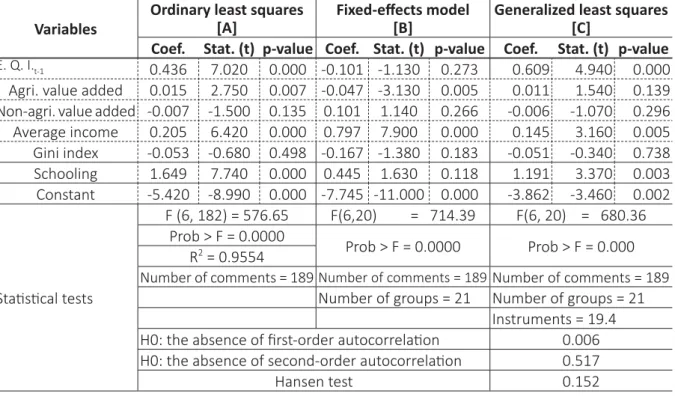
Table 4 – Results of es mates of ordinary least squares models, fi xed eff ects, and generalized least squares for the urban non-agricultural labor market
Variables
Ordinary least squares [A]
Fixed-eff ects model [B]
Generalized least squares [C]
Coef. Stat. (t) p-value Coef. Stat. (t) p-value Coef. Stat. (t) p-value
E. Q. I.t-1 0.436 7.020 0.000 -0.101 -1.130 0.273 0.609 4.940 0.000
Agri. value added 0.015 2.750 0.007 -0.047 -3.130 0.005 0.011 1.540 0.139 Non-agri. value added -0.007 -1.500 0.135 0.101 1.140 0.266 -0.006 -1.070 0.296 Average income 0.205 6.420 0.000 0.797 7.900 0.000 0.145 3.160 0.005 Gini index -0.053 -0.680 0.498 -0.167 -1.380 0.183 -0.051 -0.340 0.738 Schooling 1.649 7.740 0.000 0.445 1.630 0.118 1.191 3.370 0.003 Constant -5.420 -8.990 0.000 -7.745 -11.000 0.000 -3.862 -3.460 0.002
Sta s cal tests
F (6, 182) = 576.65 F(6,20) = 714.39 F(6, 20) = 680.36 Prob > F = 0.0000
Prob > F = 0.0000 Prob > F = 0.000 R2 = 0.9554
Number of comments = 189 Number of comments = 189 Number of comments = 189
Number of groups = 21 Number of groups = 21 Instruments = 19.4 H0: the absence of fi rst-order autocorrela on 0.006
H0: the absence of second-order autocorrela on 0.517
Hansen test 0.152
Source: survey data.
Table 5 – Results of es mates of ordinary least squares models, fi xed eff ects, and generalized least squares to the rural non-agricultural labor market
Variables
Ordinary least squares [A]
Fixed-eff ects model [B]
Generalized least squares [C]
Coef. Stat. (t) p-value Coef. Stat. (t) p-value Coef. Stat. (t) p-value
E. Q. I.t-1 0.169 2.890 0.004 0.110 2.340 0.030 0.135 3.540 0.002 Agri. value added 0.003 0.320 0.747 0.047 1.520 0.145 -0.001 -0.170 0.869 Non-agri. value added -0.001 -0.110 0.916 -0.237 -2.750 0.012 0.000 0.020 0.981 Average income 0.501 14.260 0.000 1.003 15.110 0.000 0.525 32.970 0.000 Gini index -0.309 -2.560 0.011 -0.142 -0.730 0.477 -0.330 -2.460 0.023 Schooling 0.507 5.420 0.000 0.011 0.050 0.959 0.508 6.330 0.000 Constant -4.827 -12.940 0.000 -4.732 -9.410 0.000 -4.999 -18.740 0.000
Sta s cal tests
F( 6, 182) = 351.09 F(6,20) = 323.36 F(6, 20) = 2760.56 Prob > F = 0.000
Prob > F = 0.000 Prob > F = 0.000 R2 = 0.9293
Number of comments = 189 Number of comments = 189 Number of comments = 189
Number of groups = 21 Number of groups = 21 Instruments = 19.4 H0: the absence of fi rst-order autocorrela on 0.004
H0: the absence of second-order autocorrela on 0.884
Hansen test 0.123
Source: survey data.
However, considering the levels of signifi cance of these variables for both rural and urban agricultural workers (Tables 3 and 5), note that they are sta s cally signifi cant at the level of 1%. This shows that agricultural employment responds quite diff erently to economic growth compared to non-agricultural employment. Thus, economic growth aff ects the agricultural job market, because of an increase in ac vity, whether agricultural or non-agricultural, but in a diff er-ent way. The nega ve sign result about the agricultural value added indicates that the growth in agricultural ac vi es has an inverse rela onship to the quality of employment in the two groups. This is because labor rela ons in agriculture are largely more precarious that in other sectors. Thus, as this system develops, it absorbs a por on of workers for ac vity with lower formaliza on and income, bigger workload, and higher probability of child labor occurring (characteris cs of agricultural employment), which, on average, tends to reduce the quality index of employment for that group.
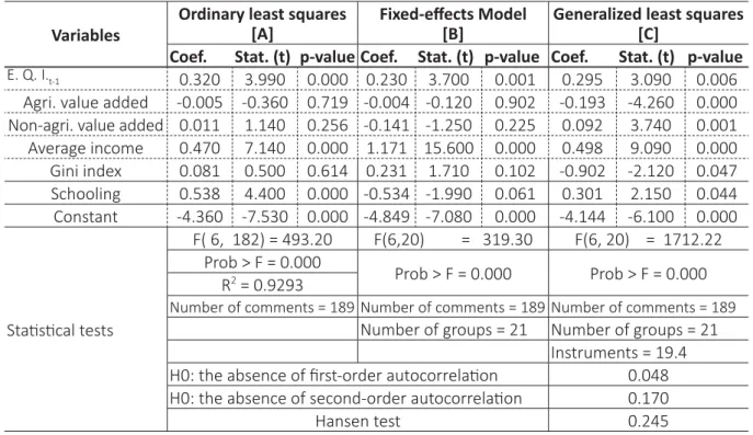
Table 6 – Results of es mates of ordinary least squares models, fi xed eff ects, and generalized least squares to the rural agricultural labor market
Variables
Ordinary least squares [A]
Fixed-eff ects Model [B]
Generalized least squares [C]
Coef. Stat. (t) p-value Coef. Stat. (t) p-value Coef. Stat. (t) p-value
E. Q. I.t-1 0.320 3.990 0.000 0.230 3.700 0.001 0.295 3.090 0.006
Agri. value added -0.005 -0.360 0.719 -0.004 -0.120 0.902 -0.193 -4.260 0.000 Non-agri. value added 0.011 1.140 0.256 -0.141 -1.250 0.225 0.092 3.740 0.001 Average income 0.470 7.140 0.000 1.171 15.600 0.000 0.498 9.090 0.000 Gini index 0.081 0.500 0.614 0.231 1.710 0.102 -0.902 -2.120 0.047 Schooling 0.538 4.400 0.000 -0.534 -1.990 0.061 0.301 2.150 0.044 Constant -4.360 -7.530 0.000 -4.849 -7.080 0.000 -4.144 -6.100 0.000
Sta s cal tests
F( 6, 182) = 493.20 F(6,20) = 319.30 F(6, 20) = 1712.22 Prob > F = 0.000
Prob > F = 0.000 Prob > F = 0.000 R2 = 0.9293
Number of comments = 189 Number of comments = 189 Number of comments = 189
Number of groups = 21 Number of groups = 21 Instruments = 19.4 H0: the absence of fi rst-order autocorrela on 0.048
H0: the absence of second-order autocorrela on 0.170
Hansen test 0.245
Source: survey data.
In the case of variable income, the es mated coeffi cient is sta s cally signifi cant at a sig-nifi cance level of 1% and with a posi ve sign, as expected, for the four equa ons examined. Thus, the increments in the income of worker have important impacts on the quality of employment. This indicates that a policy of valoriza on of real income from work can be deeply important to improve the quality standards of occupa ons and, above all, the profi le of workers. From this perspec ve, the increase in income is condi oned for jobs with be er ways of recrui ng labor. In addi on, an increase in income implies improvement of other condi ons as formaliza on, contribu on to provident ins tu ons, and increasing the quality of the occupa on. Thus, an increase in income leads to a process of compe on in the labor market. Thus, those who off er employment are encouraged to improve their hiring models to obtain workers they want and the workers feel less encouraged to remain in precarious jobs ‒ of inferior quality ‒ with lower income levels.
With regard to elas city rela ons that it can be establish, an increase of 1% on income from work has a greater impact on the quality of non-agricultural rural employment (0.53%) followed by the rural agricultural employment (0.48%). No ce that the elas city employment income quality is less than the unit and therefore, is more inelas c. Nevertheless, the idea of income recovery from work can also contribute to the reduc on of diff erences between the urban and rural labor markets, since the eff ects of income-level eleva ons at fi rst are smaller.
in terms of job quality, since the variable is inversely propor onal to the Gini EQI in all models introduced. Only in the case of urban non-farm employment does the Gini index not signifi cantly infl uence the quality of employment. Thus, non-agricultural labor rela ons are maintained with a dynamic of their own, regardless of the level of income concentra on.
Finally, it is noteworthy that the average school enrollment rate is signifi cant at a level of 1% and with a posi ve sign, according to your expected behavior within these models for the four equa ons. From this perspec ve, the level of schooling of the worker posi vely infl uences the quality of employment by increasing the possibility of the employee to obtain more
cated jobs with increases in their levels of educa on. This is consistent with the literature that deals the educa on as an inducer of work improvement.
From the perspec ve of studies of elas ci es, a 1% increase in the average educa on level of workers has a more than propor onal impact on the level of quality of the work, ceteris paribus.
This shows that investments in educa on and training are very effi cient in terms of performance and improvement of the quality of service of workers due to the elas c behavior of the quality of employment in rela on to educa on.
In the case of the variable quality of employment behind in a period, the coeffi cient is posi ve and signifi cant at a signifi cance level of 1% in the four models. Thus, the quality of em-ployment tends to persist from one year to the next, since 1% increases in quality of employ-ment passed, ceteris paribus, lead to an increase of 0.31% in urban agricultural jobs, a 0.61% increase in urban non-farm employment, a 0.13% increase in non-agricultural rural employment, and fi nally, a 0.29% increase in agricultural employment. Thus, the quality of past jobs tends to persist more strongly in non-farm employment. This is because this labor market, in addi on to being more sophis cated that the others, presents a higher level of formaliza on and incidence of labor laws, as described by Tafner (2006). The logic consists of a worker’s behavior and the dynamics of the labor market.
Generally, workers have to change their workplace if the condi ons off ered in future jobs are be er than those in current jobs. It is argued that the job market presents some resistance in terms of reducing labor achievements. Thus, generally, rights acquired are not lost over me. This behavior is refl ected in the quality of employment in that it creates some resistance when it comes to best condi ons of work already acquired. This causes the persistence of quality of employment and its infl uence on present employment.
4 FINAL CONSIDERATIONS
It is generally known that the recent transforma on of the countryside panorama has had important infl uences on labor rela ons. However, it noted be in this research that these changes go far beyond the new dynamics of produc on of the universe. The rural employment behavior obeys a number of constraints that go far beyond those in the countryside. In addi on, an urban dynamic is important to evaluate the accuracy of the trajectory of rela ons of rural work.
that the diff erences between urban and rural employment, because the rural universe persists as a more precarious environment compared to the urban environment, although the diff erences decrease with me (ESCHER et al., 2014).
Finally, it observe be from the analyses of the models that, in general, economic growth refl ects more heavily on agricultural employment than non-agricultural employment. The dynam-ics of non-agricultural ac vi es posi vely infl uence the quality level of agricultural employment to extend to these workers opportuni es for be er jobs than those in agriculture. With regard to the pace of agricultural ac vity, the ra o is reversed, and agricultural employment is generally a form of more precarious employment, depriving employees from the possibili es of achieving be er working condi ons.
In non-farm employment, this study fi nds a diff erent dynamic, recent economic growth extended the same forms of contrac ng already checked, and thus, had no major impacts in terms of structural changes on the labor markets surveyed. An important caveat must be made here: the long-term behavior of the labor market can present diff erent dynamics to those verifi ed so far, because as the economy approaches full employment induced by economic growth, the exten-sion of these forms of employment for unemployed workers becomes increasingly diffi cult. Thus, as economic growth takes place, the same result achieved in the long run is expected to cause changes in the structure of the labor market. Thus, the data refl ect the fact that labor rela ons are sensi ve to economic growth stages at the rate of economic growth itself (BALSADI, 2007).
In addi on, the survey showed that the growth of income from work and the average level of educa on of workers are important instruments not only for expanding the quality of employment level, but also as a strategy for overcoming dilemmas of the markets surveyed, as is the case with the heterogeneity observed between the groups.
REFERENCES
AHN, S. C.; SCHMIDT, P. Effi cient es ma on of models for dynamic panel data. Journal of Econometrics, v. 68, n. 1, p. 5-27, July 1995.
ALVES, C. L. B.; PAULO, E. M. Mercado de trabalho rural cearense: evolução recente a par r dos dados da PNAD. Revista da ABET, João Pessoa, PB, v. 11, n. 2, p. 47-61, jul./dez. 2012.
ARAÚJO, J. A. Pobreza, desigualdade e crescimento econômico: três ensaios em modelos de painel dinâmico. 2009. Thesis (PhD in Economics) - Federal University of Ceará (UFC), Fortaleza, 2009.
ARELLANO, M.; BOND, S. Some tests of specifi ca on for panel data: Monte Carlo evidence and an
applica on to employment equa ons. The Review of Economic Studies, v. 58, n. 2, p. 277-97, Apr. 1991. ARELLANO, M.; BOVER, O. Another look at the instrumental variable es ma on of error components model. Journal of Econometrics, v. 68, n. 1, p. 29-52, July 1995.
BALSADI, O. V. Qualidade do emprego na agricultura brasileira no período 2001-2004 e suas diferenciações por culturas. Revista de Economia e Sociologia Rural, Brasília, DF, v. 45, n. 2, p. 409-44, abr./jun. 2007. BALSADI, O. V.; DA SILVA, J. F. G. A polarização da qualidade do emprego na agricultura brasileira no período 1992-2004. Economia e Sociedade, Campinas, SP, v. 17, n. 3, p. 493-524, dez. 2008.
BALTAGI, B. H. Econometric analysis of panel data. 3rd ed. New Delh: John Wiley & Sons, 2005.
BLUNDELL, R.; BOND, S. Ini al condi ons and moment restric ons in dynamic panel data models. Journal of Econometrics, v. 87, n. 1, p. 115-43, Nov. 1998.
DA SILVA, J. G. A nova dinâmica da agricultura brasileira. 2. ed. Campinas, SP: UNICAMP, 1998.
ESCHER, F. et al. Caracterização da pluria vidade e dos plurirrendimentos da agricultura brasileira a par r do Censo Agropecuário 2006. Revista de Economia e Sociologia Rural, Brasília, DF, v. 52, n. 4, p. 643-67, out./dez. 2014.
NASCIMENTO, C. A.; BRENDA SOUTO, J. G.; OLIVEIRA, R. B.; MENDES, S. R. A qualidade do emprego rural no Estado de Minas Gerais na região Sudeste nos úl mos anos, 2002 e 2004. In: Congresso da Sociedade Brasileira de Economia Administração e Sociologia Rural, 45. Anais... Londrina: SOBER, 2007.
PAULO, E. M. Determinações do grau de qualidade do emprego: um ensaio em modelo de painel dinâmico. 2015. Masters disserta on (MD in Economics) – Federal University of Ceará (UFC), Fortaleza, 2015. SCHNEIDER, S. As novas formas sociais do trabalho no meio rural: a pluria vidade e as a vidades rurais não-agrícolas. Revista Redes, Santa Cruz do Sul, RS, v. 9, n. 3, p. 75-109, 2005.
TAFNER, P. (Ed.). Brasil: o estado de uma nação. 1. ed. Rio de Janeiro: IPEA, 2006.
WINDMEIJER, F. A fi nite sample correc on for the variance of linear effi cient two-step GMM es mators.
Journal of Econometrics, v. 126, n. 1, p. 25-51, may 2005.
Sobre os autores:
Evânio Mascarenhas Paulo: PhD. Students in Economics at Pon fi cal Catholic University
of Rio Grande do Sul and Master in Rural Economics at Federal University of Ceará. E-mail: [email protected].
Francisco José Silva Tabosa: PhD. in Economics at Federal University of Ceará and Master in Rural