www.atmos-chem-phys.net/9/6497/2009/ © Author(s) 2009. This work is distributed under the Creative Commons Attribution 3.0 License.
Chemistry
and Physics
Comparison of a global-climate model simulation to a cloud-system
resolving model simulation for long-term thin stratocumulus clouds
S. S. Lee, J. E. Penner, and M. Wang
Department of Atmospheric, Oceanic, and Space Science, University of Michigan, Ann Arbor, MI, USA Received: 16 March 2009 – Published in Atmos. Chem. Phys. Discuss.: 20 May 2009
Revised: 19 August 2009 – Accepted: 26 August 2009 – Published: 9 September 2009
Abstract. A case of thin, warm marine-boundary-layer (MBL) clouds is simulated by a cloud-system resolving model (CSRM) and is compared to the same case of clouds simulated by a general circulation model (GCM). In this study, the simulation by the CSRM adopts higher resolu-tions which are generally used in large-eddy simularesolu-tions (LES) and more advanced microphysics as compared to those by the GCM, enabling the CSRM-simulation to act as a benchmark to assess the simulation by the GCM. Ex-plicitly simulated interactions among the surface latent heat (LH) fluxes, buoyancy fluxes, and cloud-top entrainment lead to the deepening-warming decoupling and thereby the transi-tion from stratiform clouds to cumulus clouds in the CSRM. However, in the simulation by the GCM, these interactions are not resolved and thus the transition to cumulus clouds is not simulated. This leads to substantial differences in liq-uid water content (LWC) and radiation between simulations by the CSRM and the GCM. When stratocumulus clouds are dominant prior to the transition to cumulus clouds, interac-tions between supersaturation and cloud droplet number con-centration (CDNC) (controlling condensation) and those be-tween rain evaporation and cloud-base instability (control-ling cloud dynamics and thereby condensation) determine LWC and thus the radiation budget in the simulation by the CSRM. These interactions result in smaller condensation and thus smaller LWC and reflected solar radiation by clouds in the simulation by the CSRM than in the simulation by the GCM where these interactions are not resolved. The resolved interactions (associated with condensation and the transition to cumulus clouds) lead to better agreement tween the CSRM-simulation and observation than that be-tween the GCM-simulation and observation.
Correspondence to:S. S. Lee ([email protected])
1 Introduction
The formation of clouds in the marine boundary layer (MBL) is extremely important for both climate and climate sensitiv-ity (Hartmann et al., 1992; Bony and Dufresne, 2005). These clouds and the associated convection in the MBL play an im-portant role in the vertical structure of the MBL as well as air-sea fluxes of heat, moisture, and momentum (Tiedtke et al., 1988).
Aerosol concentrations have increased significantly as a result of industrialization. Increasing aerosols are generally considered to offset global warming by reflecting incom-ing solar radiation. Increasincom-ing aerosols are also known to decrease droplet size and thus increase cloud albedo (first aerosol indirect effect (AIE)) (Twomey, 1966, 1977). They may also suppress precipitation and, hence, alter LWC and lifetime (second AIE) (Albrecht, 1989). The AIE is uncer-tain, but is comparable to the radiative forcing associated with the increases in anthropogenic greenhouse gases (Ra-maswamy et al., 2001; Forster et al., 2007).
Analyses from the International Satellite Cloud Clima-tology Project (ISCCP) reveal that low-level thin strati-form clouds (with the liquid-water path (LWP)<∼50 g m−3) trapped in the MBL cover 28% of the globe. Hence, the in-terplay among these thin clouds, aerosols, and climate may have a substantial impact on climate changes and account for a large portion of the uncertainty associated with the AIE.
associated with aerosols (acting as cloud condensation nu-clei, CCN; or ice nunu-clei, IN) and hydrometeors. Many of GCMs have adopted double-moment microphysics in re-cent years by employing nucleation schemes able to calcu-late the number concentration of nucleated droplets based on local aerosol properties (e.g. size distribution, chemi-cal composition, and number concentration). This enables the prediction of cloud-particle size, an important parame-ter affecting the radiative properties of clouds as well as im-portant microphysical processes such as the autoconversion (i.e. the conversion of cloud particles to precipitable hydrom-eteors through interactions among cloud particles), collection among different classes of hydrometeors, and sedimentation of hydrometeors. However, most of these GCMs still do not take into account the dependence of collection efficiencies (controlling the autoconversion and the collection processes) and the sedimentation velocities on the size distribution of hydrometeors explicitly. They generally rely on a thresh-old cloud-liquid-water mixing ratio for the autoconversion, a fixed collection efficiency for the collection processes, and a mass-weighted fall speed for the sedimentation, so that these representations do not consider the spectral information in the size distribution. This causes uncertainties in the simula-tion of the conversion of small cloud particles to precipitable hydrometeors and in the spatial redistribution of hydromete-ors by the sedimentation. This in turn leads to uncertainties in the simulation of LWC and precipitation and thereby in the global radiation and hydrological budgets in GCMs.
This study aims to understand how the above-mentioned two lines of complication associated with cloud parameteri-zations lead to uncertainties in the simulation of microphysi-cal and radiative properties of thin, warm MBL clouds (play-ing an important role in climate and in climate changes) in GCMs. To achieve this goal, this study compares the GCM-simulated MBL clouds to those clouds GCM-simulated by a cloud-system resolving model (CSRM) for a selected region. As pointed out by Zhang et al. (2003), these two lines of compli-cation associated with cloud parameterizations can be ideally dealt with by using high-resolution models and spectrally re-solved descriptions of cloud particles and precipitable hy-drometeors for autoconversion, collection, and sedimenta-tion. Hence, by applying high-resolution grids and micro-physical parameterizations that consider the spectral infor-mation in the CSRM used in this study, the cloud properties simulated by the CSRM can act as a benchmark to assess the uncertainties and associated mechanisms (inducing those uncertainties) in GCMs.
To draw climatic implications from the comparison be-tween the GCM and CSRM simulations with better confi-dence, the comparison here is performed over the time scale associated with the approach to radiative-convective equilib-rium, which is∼three weeks (Tompkins and Craig, 1998).
2 CSRM
For numerical experiments, the Goddard Cumulus Ensemble (GCE) model (Tao et al., 2003) is used as a CSRM, which is a three-dimensional nonhydrostatic compressible model. The detailed equations of the dynamical core of the GCE model are described by Tao and Simpson (1993) and Simpson and Tao (1993).
The subgrid-scale turbulence used in the GCE model is based on work by Klemp and Wilhelmson (1978) and Soong and Ogura (1980). In their approach, one prognostic equa-tion is solved for the subgrid-scale kinetic energy, which is then used to specify the eddy coefficients. The effect of con-densation on the generation of subgrid-scale kinetic energy is also incorporated into the model.
To represent microphysical processes, the GCE model adopts the double-moment bulk representation of Saleeby and Cotton (2004). The size distribution of hydrometeors obeys a generalized gamma distribution:
n(D)= Nt
Ŵ(υ)
D
Dn
ν−1 1
Dn
exp
−D
Dn
(1) whereDis the equivalent spherical diameter (m),n(D) dD
the number concentration (m−3) of particles in the size range
dD, andNt the total number of particles (m−3). Also,νis
the gamma distribution shape parameter (non-dimensional) andDnis the characteristic diameter of the distribution (m). Full stochastic collection solutions for self-collection among cloud droplets and for rain drop collection of cloud droplets based on Feingold et al. (1988) are obtained using realistic collection kernels from Long (1974) and Hall (1980). Hence, this study does not constrain the system to a threshold mixing ratio and constant or average collection efficiencies. Following Walko et al. (1995), lookup tables are generated and used in each collection process. This enables fast and accurate solutions to the collection equations.
The philosophy of bin representation of collection is adopted for calculations of the drop sedimentation. The bin sedimentation is simulated by dividing the gamma distribu-tion into discrete bins and then building lookup tables to cal-culate how much mass and number in a given grid cell falls into each cell beneath a given level in a given time step. Thus, this study does not rely on a mass-weighted fall speed for the sedimentation. 36 bins are used for the collection and the sedimentation. This is because Feingold et al. (1999) re-ported that the closest agreement between a full bin-resolving microphysics model in a large eddy simulation (LES) of ma-rine stratocumulus cloud and the bulk microphysics repre-sentation was obtained when the collection and the sedimen-tation were simulated by emulating a full-bin model with 36 bins.
known that collection rates for droplets smaller than this size are very small, whereas droplets greater than this size partic-ipate in vigorous collision and coalescence. The large-cloud-droplet mode is allowed to interact with all other species (i.e. with the small-cloud-droplet mode and rain for warm microphysics). The large-cloud-droplet mode plays a signif-icant role in the collision-coalescence process by requiring droplets to grow at a slower rate as they pass from the small-cloud-droplet mode to rain, rather than being transferred di-rectly from the small-cloud-droplet mode to rain.
All the cloud species here have their own terminal veloc-ity. The terminal velocity of each species is expressed as power law relations (see Eq. (7) in Walko et al., 1995) based on the fall-speed formulations in Rogers and Yau (1989). A Lagrangian scheme is used to transport the mixing ratio and number concentration of each species from any given grid cell to a lower height in the vertical column, following Walko et al. (1995).
The cloud droplet nucleation parameterization of Abdul-Razzak and Ghan (2000, 2002), which is based on K¨ohler theory, is used. This parameterization combines the treat-ment of multiple aerosol types and a sectional representation of size to deal with arbitrary aerosol mixing states and arbi-trary aerosol size distributions. The bulk hygroscopicity pa-rameter for each category of aerosol is the volume-weighted average of the parameters for each component taken from Ghan et al. (2001). In applying the Abdul-Razzak and Ghan parameterization, the size spectrum for each aerosol category is divided into 30 bins.
The equation for the change in mass of droplets from the vapor diffusion (i.e. condensation and evaporation) in this study, integrated over the size distribution, is as follows:
dm
dt =Nd4π ψ FReSρvsh (2)
where Nd is the cloud droplet number concentration
(CDNC),ψthe vapor diffusivity, andρvshthe saturation wa-ter vapor mixing ratio. S is the supersaturation, given by
ρva ρvsh −1
whereρvais water vapor mixing ratio. FReis the integrated product of the ventilation coefficient and droplet diameter which is given by
FRe=
∞
Z
0
DfRefgam(D)dD (3)
where D is the diameter of droplets, fRe the ventila-tion coefficient, and fgam(D) the distribution function, given by Ŵ(υ)1 DD
n
ν−1 1
Dnexp
−D
Dn
. fRe is given by
1.0+0.229vtD
Vk
0.5
ηwherevtis the terminal velocity,Vk
the kinematic viscosity of air, and η the shape parameter (Cotton et al., 1982). In the CSRM used here, the CDNC and the supersaturation are predicted and are fed into Eq. (2) for the calculations of the condensation and the evaporation.
The parameterizations developed by Chou and Suarez (1999) for shortwave radiation and by Chou and Kouvaris (1991), Chou et al. (1999), and Kratz et al. (1998) for longwave radiation have been implemented in the GCE model. The solar radiation scheme includes absorption due to water vapor, CO2, O3, and O2. Interactions among the gaseous absorption and scattering by clouds, molecules, and the surface are fully taken into account. Reflection and transmission of a cloud layer are computed using theδ-Eddington approximation. Fluxes for a compos-ite of layers are then computed using the two-stream adding approximation. In computing thermal infrared fluxes, the k-distribution method with temperature and pressure scaling is used to compute the transmission function.
3 GCM
The GCM used here is the NCAR Community Atmospheric Model (CAM3) coupled with Integrated Massively Parallel Atmospheric Chemical Transport (IMPACT) aerosol model (CAM-UMICH) (Wang et al., 2009). The IMPACT aerosol model predicts aerosol mass for sea salt, dust, sulfate, black carbon and organic carbon (Liu et al., 2009). The original NCAR CAM3 model predicted both cloud-liquid-water mass and cloud-ice mass (Boville et al., 2006) and is updated with an additional prognostic equation for CDNC. In the coupled model, the dissipation of kinetic energy from the diffusion of momentum is calculated explicitly and included in the heat-ing applied to the atmosphere.
The aerosol model component (IMPACT) solves prognos-tic equations for sulfur and related species: dimethylsulfide (DMS), sulfur dioxide (SO2), sulfate aerosol (SO2−
4 ), and hydrogen peroxide (H2O2); aerosols from biomass burning black carbon (BC) and natural organic matter (OM), fossil fuel BC and OM, natural OM, aircraft BC (soot), mineral dust, and sea salt are also included. Sulfate aerosol is divided into three size bins with radii varying from 0.01–0.05µm, 0.05–0.63µm and 0.63–1.26µm, while mineral dust and sea salt are predicted in four bins with radii varying from 0.05– 0.63µm, 0.63–1.26µm, 1.26–2.5µm, and 2.5–10µm (Liu et al., 2009). Carbonaceous aerosol (OM and BC) is cur-rently represented by a single submicron size bin. Emis-sions of primary particles and precursor gases, gas-phase ox-idation of precursor gases, aqueous-phase chemistry, rain-out and washrain-out, gravitational settling, and dry deposition are treated. The mass-only version of the IMPACT aerosol model driven by meteorological fields from the NASA Data Assimilation Office (DAO) participated in the AEROCOM (http://nansen.ipsl.jussieu.fr/AEROCOM/) phase A and B evaluations (Textor et al., 2006), where it has been exten-sively compared with in situ and remotely sensed data for different aerosol properties.
al. (2006) and Collins et al. (2006). The shallow stratiform clouds, which is the cloud type of interest to us here, are pa-rameterized following the Rasch and Kristj´ansson’s (1998) treatment modified by Zhang et al. (2003). In this parameter-ization, the net stratiform condensation of cloud liquid wa-ter (condensation minus evaporation) is diagnosed based on environmental conditions such as temperature, water vapor, cloud-liquid-water mixing ratio, and cloud fraction. This is different from the condensation scheme used in the CSRM (described in Sect. 2) where the condensation is explicitly calculated based on predicted variables such as the super-saturation and the CDNC. The conversion of cloud liquid water to rain (through autoconversion and collection pro-cesses between cloud liquid water and rain) follows Boucher et al. (1995) and Tripoli and Cotton (1980), using a thresh-old mixing ratio and a constant collection efficiency with no consideration of the spectral hydrometeor information.
The standard CAM3 version has been updated with a prog-nostic equation for CDNC, which replaces the prescribed CDNC used in the standard CAM3. This prognostic CDNC equation treats droplet source from aerosol particle activation and convective detrainment, and droplet sinks from evapora-tion, self-collecevapora-tion, and precipitation. The droplet activa-tion is parameterized based on K¨ohler theory (Abdul-Razzak and Ghan, 2000, 2002), the same as that used in the CSRM. The droplet self-collection is based on the treatment of Be-heng (1994), droplet depletion by precipitation and evapora-tion is assumed to be proporevapora-tional to the depleevapora-tion of LWC.
The coupled system is run with 26 vertical levels and a 2◦
×2.5◦horizontal resolution. In the MBL, the vertical grid
length is∼300–600 m. This system is run in MPMD
(Mul-tiple Processors Mul(Mul-tiple Data) mode to exchange aerosol fields and meteorological fields at each advection time step of the IMPACT model. The finite volume dynamical core was chosen for the NCAR CAM. This version of the coupled model participated the AeroCOM indirect effect intercom-parison project, where the simulated aerosol/cloud relation-ships have been extensively compared with satellite and field data.
4 Integration design of the CAM-UMICH model
A simulation is carried out with the present-day (PD) aerosol emissions using the coupled CAM-UMICH model. This sim-ulation is referred to as the “GCM run”, henceforth. The GCM run is integrated for 1 year after an initial spin-up of four months. The time step for CAM3 is 30 min, and that for advection in IMPACT is 1 h. The aerosol fields are assumed not to have any direct effect on the simulated meteorological fields.
Anthropogenic sulfur emissions are from Smith et al. (2001, 2004), and those for the year 2000 are used. Anthropogenic emissions of fossil fuel and biomass burn-ing carbonaceous aerosols were from Ito and Penner (2005)
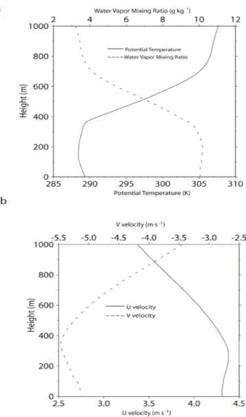
Fig. 1.Vertical profiles of(a)initial potential temperature and water vapor mixing ratio and(b)initial horizontal wind (u, v) velocity for the CSRM run.
1366
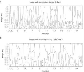
Fig. 2. Time-height cross section of (a) potential temperature large-scale forcing (K day−1) and(b)humidity large-scale forcing (g kg−1day−1) for the CSRM run. Contours start at 0 and the con-tour interval is 5.
5 Case descriptions and integration design of the CSRM
MBL stratocumulus clouds develop at (30◦N, 120◦W) off
the coast of the western Mexico from∼30 June to∼20 July in the GCM run. These clouds are selected for a comparison between the GCM and CSRM simulations.
For the CSRM simulation (referred to as the “CSRM run” henceforth), initial conditions, large-scale forcings of humid-ity and temperature, and surface fluxes are extracted from the GCM run from 16:00 LST (local solar time) on 30 June to 16:00 LST on 20 July at (30◦N, 120◦W). These extracted
environmental conditions are imposed on the CSRM run so that the CSRM run can be performed under the same envi-ronmental conditions as those in the GCM run. The large-scale forcings of humidity and temperature and surface fluxes are extracted every 3 h. The 3-hourly data are applied to the CSRM at every time step by interpolation. The time step of the CSRM run is 0.5 s. The horizontally averaged wind from the GCE model is nudged toward the interpolated wind field from the GCM run at every time step with a relaxation time of one hour, following Xu et al. (2002). The large-scale terms are approximated to be uniform over the model domain and they are defined to be functions of height and time only, following Krueger et al. (1999). This method of modeling cloud systems was used for a CSRM comparison study by Xu et al. (2002). The details of the procedure for applying large-scale forcings and surface fluxes are described in Don-ner et al. (1999) and are similar to the method proposed by Grabowski et al. (1996).
Fig. 3. Time series of surface sensible (SH) and latent (LH) heat fluxes (W m−2)(a)for the CSRM run and(b)time series of LH surface fluxes for the CSRM-LH run.
Vertical profiles of initial specific humidity, potential tem-perature, and horizontal wind velocity applied to the CSRM run are shown in Fig. 1 and large-scale forcings and surface fluxes imposed on the CSRM are depicted in Figs. 2 and 3a, respectively. The profiles of humidity and potential tempera-ture indicate that the initial inversion layer is formed around 400 m. Below the inversion layer,u(wind in the east-west di-rection) andv (wind in the north-south direction) velocities do not vary much as the humidity and the potential tempera-ture. The plus and minus indicate eastward (northward) and westward (southward) wind direction for theu (v) veloci-ties. The large-scale forcings show the diurnal variation. The sensible heat (SH) fluxes do not vary significantly, whereas the latent heat (LH) fluxes increase significantly after around 00:00 LST 13 July. Figure 3b depicts the latent heat fluxes used in a supplementary simulation which will be discussed in more detail in Sect. 6.3.
The CSRM run is performed in a 3-D framework. A uni-form grid length of 50 m is used in the horizontal domain and the vertical grid length is uniformly 20 m below 3 km and then stretches to 480 m near the model top. Periodic bound-ary conditions are set at the horizontal boundaries.
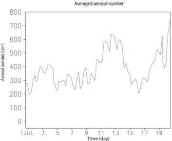
Fig. 4. Time series of background aerosol number concentration (cm−3) averaged over the MBL in the CSRM run.
we used 1000 parallel CPUs for such a computation. These CPU hours are∼2 times larger than total hours assigned to the entire set of climate groups in the National Energy Re-search Scientific Computing (NERSC) center (whose super-computer system is used for this study) in the year 2008. Also, it should be pointed out that the total wall-clock time needed for this simulation is∼7 years despite the use of 1000 CPUs. Hence, a compromise is needed by finding a domain size which is large enough to simulate the MBL clouds rea-sonably yet small enough to enable us to perform simulations within the given computer resources and within a reasonable well-clock time range.
Various field experiments performed in both clear and cloudy boundary layers have shown that generally a signifi-cant amount of variance in large-scale disturbances (whose spatial scale is comparable to the size of the GCM grid box) is present at the mesoscale spatial scale for quanti-ties such as moisture, temperature, or the horizontal wind components (e.g. Nicholls and LeMone, 1980; Rothermel and Agee, 1980; Nucciarone and Young, 1991; Davis et al., 1996; Jonker et al., 1997; Young, 1987; Durand et al., 2000). de Roode et al. (2004) reported that the spatial scale of mesoscale fluctuations was∼10–20 km in general. Based on this, the horizontal domain length is set to 12 km in both the east-west and north-south directions in this study to cap-ture the mesoscale struccap-tures whose properties can be as-sumed to represent those of the large-scale disturbances rea-sonably well. The vertical domain length is 20 km to cover troposphere and the lower stratosphere. To make a consis-tency in radiation between the CSRM and the GCM above 20 km (the GCM vertical domain extends to the pressure level of 3 hPa, corresponding to∼40 km), additional layers
representing atmospheric conditions above 20 km are applied only to radiation scheme in the CSRM run as described in Tao et al. (2003).
Xiping et al. (2007) compared a 20-day cloud simulation of a CSRM to observations by applying observed initial con-ditions, large-scale forcings, and surface fluxes to the CSRM. Similarly, this study compares the CSRM run to the GCM run by applying environmental data (produced by the GCM) to the CSRM adopted here. These GCM-produced data are 3 hourly (the same as the observed data in Xiping et al. (2007)) and collected with a similar vertical resolution to that in ob-served data in Xiping et al. (2007). This enables a similar comparison of the CSRM run to the GCM run to the com-parison of the CSRM simulation to observations in Xiping et al. (2007). The GCM run in this study is analogous to the observations in Xiping et al. (2007), since it provides the environmental conditions to the simulation by the CSRM here. However, in Xiping et al. (2007), observations acted as a benchmark to evaluate the performance of the CSRM, whereas, in this study, the CSRM run is intended to act as a benchmark to evaluate the GCM run by applying the higher resolution and advanced microphysics to the CSRM used here.
Background aerosol data for the CSRM run are provided by the coupled CAM-UMICH model from 16:00 LST on 30 June to 16:00 LST on 20 July at (30◦N, 120◦W). Hence,
the CSRM run is under the same background aerosol condi-tions as those in the GCM run. The predicted aerosol mass of each aerosol species by the GCM run is obtained every 6 h. These mass data are interpolated into every time step to up-date the background aerosols in the CSRM run. The aerosol mass is approximated to be uniform over the model horizon-tal domain and is defined to be a function of height and time only.
Aerosol number concentration is calculated from the mass profiles using parameters (mode radius, standard deviation, and partitioning of aerosol number among modes) described in Chuang et al. (1997) for sulfate aerosols and Liu et al. (2005) for non-sulfate aerosols (e.g. fossil fuel BC/OM, biomass BC/OM, sea salt, and dust) as in the GCM runs. Here, bi- or tri-modal log-normal size distribution is as-sumed for aerosols and the number of aerosols in each size bin of the distribution is determined using these parameters and assumed aerosol particle density for each species. In the MBL, background aerosol number is nearly constant and only varies vertically within 10% of its value at the surface. The time series of the vertically averaged total background aerosol number over the MBL in the CSRM run is shown in Fig. 4. Generally, the aerosol number varies between 200 and 700 cm−3, indicating that these aerosols correspond to typical clean continental aerosols (Whitby, 1978).
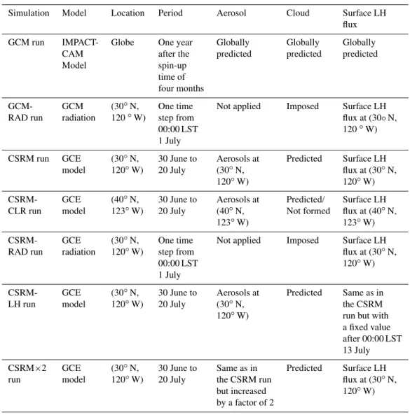
Table 1.Summary of simulations.
Simulation Model Location Period Aerosol Cloud Surface LH flux
GCM run IMPACT- Globe One year Globally Globally Globally
CAM after the predicted predicted predicted
Model spin-up
time of four months
GCM- GCM (30◦N, One time Not applied Imposed Surface LH
RAD run radiation 120◦W) step from flux at (30◦N,
00:00 LST 120◦W)
1 July
CSRM run GCE (30◦N, 30 June to Aerosols at Predicted Surface LH
model 120◦W) 20 July (30◦N, flux at (30◦N,
120◦W) 120◦W)
CSRM- GCE (40◦N, 30 June to Aerosols at Predicted/ Surface LH CLR run model 123◦W) 20 July (40◦N, Not formed flux at (40◦N,
123◦W) 123◦W)
CSRM- GCE (30◦N, One time Not applied Imposed Surface LH
RAD run radiation 120◦W) step from flux at (30◦N,
00:00 LST 120◦W)
1 July
CSRM- GCE (30◦N, 30 June to Aerosols at Predicted Same as in
LH run model 120◦W) 20 July (30◦N, the CSRM
120◦W) run but with
a fixed value after 00:00 LST 13 July
CSRM×2 GCE (30◦N, 30 June to Same as in Predicted Surface LH run model 120◦W) 20 July the CSRM run flux at (30◦N,
but increased 120◦W)
by a factor of 2
droplets (nucleation scavenging). Initially, the aerosol num-ber is set equal to its background value everywhere.
Table 1 summarizes simulations in this study. In addi-tion to the GCM run and the CSRM run, Table 1 shows that supplementary simulations are performed. They will be de-scribed in more detail in the following sections.
This study focuses on aerosol effects on the nucleation of cloud particles and thereby cloud microphysical and radiative properties and, thus, does not take into account aerosol direct effects on radiation. In other words, only aerosol impacts on cloud-particle properties after its activation are taken into account for both the GCM run and the CSRM run.
6 Results
6.1 Clear-sky case
1390
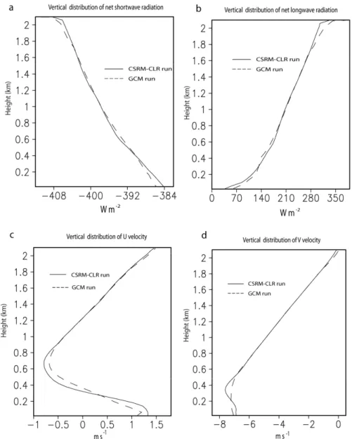
Fig. 5.Vertical distribution of the time- and area-averaged(a)net shortwave fluxes,(b)net longwave fluxes,(c)uwind velocity,(d)vwind velocity,(e)potential temperature,(f)pressure,(g)water-vapor mixing ratio, and(h)aerosol number concentration for the CSRM-CLR run and the GCM run at (40◦N, 123◦W). In (a) and (b), plus and minus indicate upward and downward fluxes, respectively.
To show this robustness, a CSRM simulation for a clear-sky case is simulated. Henceforth, this CSRM simulation is referred to as the CSRM-CLR run. A region at (40◦
N, 123◦
W) where no clouds are formed over a 20-day period (16:00 LST on 30 June to 16:00 LST on 20 July) in the GCM run is selected for the CLR run. The CSRM-CLR run is identical to the CSRM run but the initial con-ditions, the large-scale forcings, and the surface fluxes pro-duced by the GCM run at (40◦N, 123◦W) are used.
Com-paring the CSRM-CLR run to the GCM run in the absence of clouds enables a test of the robustness to the differences in schemes other than schemes for clouds, since those schemes for clouds are not activated in the clear-sky case.
Fig. 6.Time series of domain-averaged (over the lowest 2 km)(a)net shortwave fluxes,(b)net longwave fluxes,(c)uwind velocity,(d)v wind velocity,(e)potential temperature,(f) pressure,(g)water-vapor mixing ratio, and(h)aerosol number concentration for the CSRM-CLR run and the GCM run at (40◦N, 123◦W). In (a) and (b), minus and plus indicate downward and upward fluxes, respectively.
demonstrates that we are able to assume that the results of this study are not significantly sensitive to the schemes not associated with clouds. This in turn enables us to assume that differences in the results for a cloud case between the CSRM run and the GCM run are mostly attributable to differences in cloud schemes.
In the case of radiation schemes, the prescription of pa-rameters for the radiative properties of cloud particles is different between the CSRM and the GCM adopted here. Hence, it is necessary to show that radiation schemes do not show significant differences in the responses to identi-cal clouds, though radiation schemes do not show significant differences in the clear-sky case. If there are insignificant differences in the radiation for identical clouds, the different prescriptions of radiative parameters within clouds can be as-sumed to not contribute to differences between the CSRM run and the GCM run. In other words, it is the different cloud properties (e.g. LWC and effective size) due to dif-ferent cloud schemes (but not the difdif-ferent prescription of radiative parameters) that contribute to differences in radi-ation, if the radiation schemes respond similarly to identi-cal clouds. To test the responses of the radiation schemes to identical clouds, idealized simulations are carried out.
For these simulations, the radiation schemes are separated from the CSRM and the GCM and the initial meteorologi-cal conditions of the CSRM run and the GCM run at (30◦N,
120◦W) are fed into those radiation schemes. These
simula-tions are performed within a 1-D framework for just one time step, which is 0.5 s. The model domain has only the vertical domain whose depth is 20 km. For these radiation schemes, a cloud layer, with a homogeneous cloud-liquid-water mixing ratio and effective size throughout the cloud layer, between 200 m and 400 m is imposed. The vertical extent of cloud layer is based on stratocumulus clouds which are generally simulated in a layer between 200 m and 400 m in the CSRM run and GCM run at (30◦N, 120◦W); these simulated clouds
Table 2. Time- and area-averaged net shortwave radiation flux (SW) and longwave radiation flux (LW) at 20 km (TOA) and base (SFC) of the atmosphere for the CSRM-RAD run and the GCM-RAD run.
Shortwave flux (SW) and longwave flux (LW)
at 20 km (TOA) and base (SFC) of the model in the CSRM-RAD run and the GCM-RAD run (W m−2)
Effective Cloud-liquid- TOA SW TOA LW SFC SW SFC LW
radius (µm) water mixing ratio (g kg−1)
CSRM GCM CSRM GCM CSRM GCM CSRM GCM
radiation radiation radiation radiation radiation radiation radiation radiation
5 0.01 −707.7 −680.7 314.1 325.2 −582.9 −562.3 98.1 103.1
5 0.05 −641.7 −610.2 312.6 319.6 −513.0 −500.2 65.4 69.2
5 0.2 −492.6 −480.5 310.4 316.1 −354.2 −342.1 26.8 29.1
5 0.4 −396.6 −387.5 309.5 315.9 −251.2 −245.2 18.3 20.3
5 0.6 −344.4 −340.1 309.0 315.3 −194.8 −190.3 15.2 17.1
15 0.01 −711.7 −691.3 314.2 325.1 −585.9 −565.6 99.4 104.2
15 0.05 −657.8 −620.5 312.8 319.2 −525.0 −512.1 70.4 75.6
15 0.2 −526.3 −510.3 310.2 316.8 −378.4 −367.1 28.9 30.2
15 0.4 −434.2 −425.2 309.5 315.6 −275.9 −269.5 18.6 20.5
15 0.6 −382.2 −375.1 309.0 315.2 −216.5 −211.7 16.3 18.0
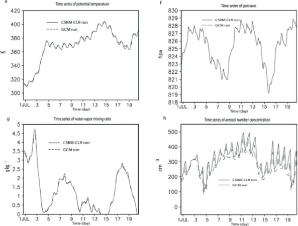
Fig. 7. Time-height cross section of cloud-liquid-water mixing ra-tio (g kg−1) for(a)the CSRM run,(b)the GCM run, and(c)the CSRM-LH run. Contours are at 0.01, 0.4, and 0.6 g kg−1.
Table 2. For each combination, a simulation is carried out with the CSRM radiation scheme (henceforth, referred to as the “CSRM-RAD run”) and the simulation is repeated with the GCM radiation scheme (henceforth, referred to as the “GCM-RAD run”). Table 2 shows the net shortwave and longwave radiation fluxes at 20 km (TOA) and the surface (SFC) for the CSRM-RAD run and the GCM-RAD run for each of the combinations of mixing ratios and effective radii. Those fluxes for the CSRM-RAD run are within ∼10% of those for the GCM-RAD run; this also holds for the individ-ual upward and downward fluxes (not shown). Hence, those radiation schemes can be considered to show nearly identical responses to identical clouds and this supports the assump-tion that differences in simulaassump-tions between the CSRM run and the GCM run are mostly caused by differences in cloud schemes.
6.2 Cloud properties and comparison with observation
Figures 7a and b show the time-height cross section of cloud-liquid-water mixing ratio for the CSRM run and the GCM run. Figure 8a shows the time series of the liquid-water paths (LWPs) for those runs, which are smoothed over 1 day (av-eraged over the period between 12 h before and after a time point), and those observed by the Moderate Resolution Imag-ing Spectroradiometer (MODIS) on the Terra satellite, which are provided as an averaged values over one-day period (for the 10:30 a. m. and 10:30 p. m. crossing times for July 2001 to 2008).
1414
Fig. 8.Time series of(a)LWP (g m−3) averaged over the horizon-tal domain and(b)effective radius (micron) conditionally averaged over the cloudy regions for the CSRM run, the GCM run, and the MODIS observation.
GCM run. The LWP in the GCM run generally shows much larger temporal fluctuations than the MODIS-observed LWP and the CSRM-run LWP.
Figure 8b shows the time series of effective radius of cloud liquid water, conditionally averaged over cloudy regions for the GCM run and the CSRM run, smoothed over 1 day. The MODIS observation of the one-day averaged effective radius is also plotted for comparison. In general, the CSRM-run effective size is closer to the MODIS-observed size than the GCM-run size. For the calculation of the conditional aver-age over the cloudy regions, one needs to determine the grid points within the cloud. Grid points are assumed to be in cloud if the number concentration and volume-mean size of droplets is typical for clouds and fogs (1 cm−3or more, 1µm or more; Pruppacher and Klett, 1997). The conditional aver-age over the grid points in cloud is obtained at each time step; the conditional average is the arithmetic mean of the variable over the collected grid points in cloud (grid points in clear air are excluded from the collection).
It should be noted that there is an uncertainty associated with the retrieval of the MODIS LWP and droplet size. Gen-erally, the retrieval errors are ∼10% for LWP and droplet
size according to Ju´arez et al. (2009). Hence, the qualita-tive nature of the differences in LWP and droplet size among the CSRM run, the GCM run, and the MODIS observation shown here is not likely to depend on the uncertainty.
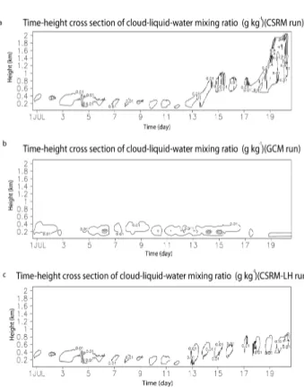
Fig. 9.Contours of cloud-liquid-water mixing ratio (g kg−1) at the time of the occurrence of maximum depth of the averaged cloud-liquid-water mixing ratio (03:00 LST 19 July) along the x (east-west) direction in the middle of the y (north-south) direction in the CSRM run. Contours are at 0.05, 0.2, 0.4, and 0.6 g kg−1.
Around 00:00 LST on 13 July, cloud depth and height start to increase in the CSRM run, whereas they do not show sig-nificant changes in the GCM run (Fig. 7a and b). Around 00:00 LST on 17 July, the depth of the domain-averaged cloud-liquid-water mixing ratio start to increase substantially and the cloud tops reach∼2 km around 03:00 LST on 19 July
Fig. 10. Time series of BIR averaged over the horizontal domain for the CSRM run.
is downward, at the TOA and the SFC) in the CSRM run after 00:00 LST on 17 July despite the generally larger droplet size in the CSRM run than in the GCM run after 00:00 LST on 17 July (Fig. 8b). The cloud fraction averaged over all the time steps and a layer between minimum cloud-base height and maximum cloud-top height in the CSRM (GCM) run af-ter 00:00 LST 17 July is 0.75 (0.55). At time steps when clouds are absent, the lifting condensation level (LCL) and the MBL top replace the minimum cloud-base height and maximum cloud-top height, respectively, for the calculation of the cloud fraction. Thus the larger cloud fraction asso-ciated with the transition to cumulus clouds contributes to larger upward shortwave radiation at the TOA in tandem with the LWP in the CSRM run after 00:00 LST 17 July. The area-averaged net shortwave radiation at the TOA and the SFC after 00:00 LST 17 July are−322.5 (−430.2) and
−202.8 (−320.2) W m−2 in the CSRM (GCM) run,
respec-tively. Note that a minus indicates the downward fluxes. Next, an analyses of the mechanisms that induce the tran-sition from the stratocumulus clouds to the cumulus clouds in the CSRM run is discussed.
6.3 Transition from stratocumulus to cumulus
Figure 10 shows the time series of the buoyancy integral ra-tio (BIR) of Bretherton and Wyant (1997) (hereafter BW97) (see Eq. (14) in BW97 for the details of the BIR) in the CSRM run. The BIR is defined as the ratio of the integral of the magnitude of buoyancy fluxes over the regions of neg-ative buoyancy below cloud base to the integral of the buoy-ancy fluxes over all other regions. For the calculation of the BIR, when clouds are absent, the LCL replaces the cloud base. Figure 7a shows cloud thinning or clearing due to the
Fig. 11. Vertical distribution of the time- and area-averaged buoyancy fluxes (K m s−1)(a)over 16:00 LST 30 June–00:00 LST 13 July,(b)over 00:00 LST 13 July–00:00 LST 17 July, and(c)over 00:00 LST 17 July–16:00 LST July.
decoupling between the cloud layer and the sub-cloud layer driven by shortwave heating during the daytime when the stratocumulus is a dominant cloud type prior to 00:00 LST on 17 July. After the sun sets, longwave cooling at the cloud top revitalizes convection with the reduction of the magni-tude of the decoupling.
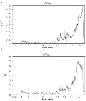
Fig. 12.Time series of averaged(a)1qtBL(g kg−1) and(b)1θ tBL (K) over the horizontal domain for the CSRM run.
as shown in Fig. 11 depicting the vertical distribution of the averaged buoyancy fluxes over three time periods (16:00 LST 30 June–00:00 LST 13 July, 00:00 LST 13 July–00:00 LST 17 July, and 00:00 LST 17 July–16:00 LST 20 July). The buoyancy fluxes are calculated in the same manner as those in Jiang et al. (2002). The negative buoyancy flux is not present in the first time period (when the stratocumulus clouds with low bases are dominant) in Fig. 11a, indicating that decou-pling is not active. A large increase in the negative buoyancy flux is shown in the second time period (when the cloud-bases of stratocumulus clouds start to increase) in Fig. 11b, indicating the occurrence of decoupling. The negative buoy-ancy flux reaches its maximum in the third time period (when cumulus clouds begin to develop and become a dominant cloud type), indicating the most active decoupling.
The degree of decoupling can also be assessed by sim-ply estimating the vertical stratification of the total water mixing ratio (qt; the sum of water-vapor mixing ratio and cloud-liquid-water mixing ratio) and the potential tempera-ture (θ) following BW97. Starting with the horizontal mean soundings (denoted by<qt>and<θ >), the vertical
aver-ages of each in a 75-m thick layer at the surface and in a 75-m thick layer just below the inversion, we define “1qtBL” and “1θBL” as the differences in <qt>and<θ >, respectively,
between the surface and the boundary-layer (BL) top:
1qtBL≡<qt>surface−<qt>BLtop (4)
Fig. 13. Time series of averaged (over the horizontal domain) net radiative flux divergence (W m−2) over the cloud layer (solid line) and over the sub-cloud layer (dashed line) for the CSRM run. When clouds are not present, the cloud layer is defined as the layer be-tween the LCL and the MBL top.
1θtBL≡<θ >surface−<θ >BLtop (5) Increasing “1qtBL” or “1θtBL” indicates more decoupling and internal BL stratification. Figure 12 shows both “1qtBL” and “1θtBL” remain small and relatively constant up to 00:00 LST on 13 July. This indicates that a well-mixed boundary layer is maintained up to 00:00 LST on 13 July (associated with the development of stratocumulus clouds with low bases as shown in Fig. 7a). But, they increase rapidly around 00:00 LST on 13 July when the cloud-base height starts to increase and more rapidly around 00:00 LST on 17 July when cumulus clouds begin to develop, indicating strong decoupling. BW97 pointed out that decoupling (lead-ing to cumulus formation) is mainly due to the increas(lead-ing latent heat fluxes at the surface.
Figures 3a and 13 depict the time series of the surface fluxes and the radiative flux divergence (one of the diabatic forcings) for the CSRM run, respectively. The most obvi-ous trend is that the LH flux starts to increase with time around 00:00 LST on 13 July when the cloud-base height and BIR start to increase substantially; prior to 00:00 LST on 13 July, the LH flux does not either increase or decrease significantly. The net radiative flux divergence across the cloud layer of the combined longwave and shortwave radi-ation is 1FR=FR+−FR(zb). Here, FR is the net radiation
flux where plus and zb denote the cloud top and base,
Fig. 14.Time series of area-averaged precipitation rate (mm day−1) at cloud base (or at the LCL when clouds are absent) (solid line) and at the surface (dashed line) for the CSRM run.
of the radiative flux divergence does not vary significantly prior to 00:00 LST on 13 July when the decoupling starts to occur. The divergence across the sub-cloud layer, which is
1FR=FR(zb)−FR(0)(where 0 denotes the surface) , is less
than∼2 W m−2prior to 00:00 LST on 13 July (Fig. 13). This indicates a slight radiative warming of the subcloud layer. The diurnal cycle of precipitation at cloud base (or at the LCL when clouds are absent) also does not vary significantly, indicating that the latent heating in the cloud layer due to the formation of precipitation does not vary much prior to 00:00 LST on 13 July (Fig. 4). All precipitation evaporates before reaching the surface, leading to no surface precipi-tation prior to 00:00 LST on 13 July (Fig. 14). Thus, the net latent heating of the MBL due to precipitation is zero prior to 00:00 LST on 13 July. The evaporation of precipita-tion substantially reduces the difference between the diabatic cooling in the cloud layer and that below, inhibiting the com-pletion of convection from the surface to the MBL top and promoting decoupling. However, the diabatic cooling (in the cloud and sub-cloud layers) does not change greatly during the coupled phase as shown in Figs. 13 and 14. This indi-cates that diabatic forcings do not explain the occurrence of decoupling. The large-scale temperature and humidity forc-ings also do not show substantial changes up to 00:00 LST on 13 July (Fig. 2). Figure 15 shows the area-averaged large-scale vertical velocity at the MBL top and it does decrease around 00:00 LST on 13 July, which is when the increase in subsidence occurs. This counters the increase in cloud-base and -top heights around 00:00 LST on 13 July.
The above analyses of the variables associated with the MBL energy budgets and the large-scale subsidence indicate that the surface LH flux is a primary candidate for strong
Fig. 15. Time series of area-averaged large-scale vertical velocity (w) (cm s−1) at the MBL top for the CSRM run.
Fig. 16.Time series of the cloud-layer averaged LH fluxes for the CSRM run. When clouds are not present, the cloud layer is defined as a layer between the LCL and the MBL top.
averaged latent heat flux. Here, when clouds are not present, the cloud layer is defined as a layer between the LCL and the MBL top as in the calculation of the radiative diver-gence. The averaged latent heat fluxes start to increase sub-stantially around 00:00 LST on 13 July when the surface LH fluxes start to increase, contributing to the increase in in-cloud buoyancy fluxes and thus the buoyancy jump around the cloud base and the decoupling as shown in Fig. 11b. This supports the leading role of the LH fluxes in the development of decoupling and cumulus clouds.
As reported in BW97 and shown in this study, upward latent heat fluxes in the boundary layer increase with an increase in the surface latent heat fluxes. This increases the buoyancy fluxes and turbulence levels within the cloud, creating more entrainment per unit of cloud radiative cool-ing. The increased entrainment leads to increasingly neg-ative buoyancy fluxes below cloud base associated with a downward flux of warm entrained air as shown in Fig. 11b. BW97 explained that this disrupted the mixed layer and cre-ated a weak stable layer below cloud base, leading to the de-velopment of conditionally unstable cloud layer. The stable layer acted as a valve that allowed only the most powerful subcloud-layer updrafts to penetrate up to the main stratocu-mulus cloud base, leading to the development of custratocu-mulus clouds. As the decoupling became more pronounced, the cu-mulus clouds developed more.
To confirm the major role of the latent heat fluxes in the development of strong decoupling and cumulus clouds, an additional simulation is performed. This simulation is iden-tical to the CSRM run except that a different surface latent heat flux is applied after 00:00 LST on 13 July. Figure 3b de-picts the latent heat flux applied to this additional simulation (henceforth, referred to as the “CSRM-LH” run). As seen in the comparison between Fig. 3a and b, the surface latent heat flux does not increase and is set to the same value as at 00:00 LST on 13 July for this additional simulation after 00:00 LST on 13 July when cloud-base and -top heights both start to increase in the CSRM run. As seen in Fig. 7c, cu-mulus clouds do not develop after 00:00 LST 17 July in this simulation, supporting the notion the increase in the surface latent heat flux is the impetus for the development of strong decoupling and cumulus clouds after 00:00 LST on 13 July. 6.4 Liquid-water budget of stratocumuls clouds in the
CSRM run
A smaller LWC and thus LWP is simulated in the CSRM run than that in the GCM run from 16:00 LST on 30 June to 00:00 LST on 17 July before the development of cumu-lus. The time- and domain-averaged LWP prior to 00:00 LST on 17 July is 24.3 and 10.3 g m−2for the GCM run and the CSRM run, respectively. This contributes to a smaller up-ward shortwave radiation at the TOA and thus a larger mag-nitude of the net shortwave radiation, which is downward, at TOA and SFC, respectively, despite the smaller droplet size
(Fig. 8b) and larger cloud fraction in the CSRM run than in the GCM run. The averaged cloud fraction is 0.61 (0.59) in the CSRM (GCM) run. The cloud fraction here is calculated in the same manner as explained in Sect. 6.2 except that the average is over the period between 16:00 LST on 30 June and 00:00 LST on 17 July. The time- and area-averaged net short-wave radiation flux at the TOA and the SFC over the period between 16:00 LST on 30 June and 00:00 LST on 17 July are
−423.6 (−324.3) and−351.2 (−193.5) W m−2in the CSRM (GCM) run, respectively.
The smaller LWC in the CSRM run than in the GCM run leads to a better agreement in the LWP between the CSRM run and the MODIS observation. The time-averaged LWP prior to 00:00 LST on 17 July is 12.3 g m−2for the MODIS observation.
The LWPs prior to 00:00 LST on 17 July are less than 50 g m−2. Hence, stratocumulus clouds here can be con-sidered thin according to the classification of Turner et al. (2007). As shown in Lee et al. (2009), condensation plays a critical role in the determination of the LWC and LWP in thin clouds. Other processes such as autoconversion, collec-tion, and sedimentation play a negligible role in the determi-nation of the LWC and LWP.
To elucidate the microphysical processes controlling the LWC and LWP of the stratocumulus clouds in the CSRM run before the development of cumulus clouds, domain-averaged cumulative sources (i.e. condensation) and sinks of cloud liq-uid water (the small-cloud-droplet mode + the large-cloud-droplet mode) were obtained. For this, the production equa-tion for cloud liquid water is integrated over the domain and over the period between 16:00 LST 30 June and 00:00 LST 17 July. Those integrations are denoted by< >:
<A>= 1
LxLy
RRR
ρaAdxdydzdt (6)
whereLxandLyare the domain length (12 km), in east-west and north-south directions, respectively. ρa is the air
den-sity andArepresents any of the variables in this study. The budget equation for cloud liquid water is as follows:
<∂qc
∂t >=<Qcond>−<Qevap>−<Qauto>−<Qaccr> (7)
0.033 0.34 0.30 0.00024 0.0071 mm
Here,qcis cloud-liquid-water mixing ratio. Qcond,Qevap,
Qauto, andQaccrrefer to the rates of condensation, evapora-tion, autoconversion of cloud liquid water to rain, and accre-tion of cloud liquid water by rain, respectively.
The budget numbers beneath Eq. (7) show that condensa-tion and evaporacondensa-tion are∼one to three orders of magnitude larger than autoconversion and accretion as also shown in Lee et al. (2009). This indicates that the conversion of cloud liquid water (produced by condensation) to rain is highly in-efficient.
is mainly controlled by the sedimentation of cloud parti-cles larger than the critical size for collisions around∼20–
∼40µm in radius (Pruppacher and Klett, 1997). Cloud mass here is the sum of the mass of all species associated with warm microphysics, i.e. the small-cloud-droplet mode, the large-cloud-droplet mode, and rain. Autoconversion and ac-cretion are processes that control the growth of cloud par-ticles after they reached around the critical size or larger (Rogers and Yau, 1989). Hence, the small contribution of autoconversion and accretion to the LWC implies that the role of sedimentation of cloud particles in the determination of the LWC is not as significant as that of condensation and evaporation.
Figure 17a and b show the time- and area-averaged verti-cal distribution of condensation and cloud-mass changes due to sedimentation over the period before the development of cumulus clouds for the CSRM run. The vertical coordinate is in the units of the height normalized with respect to the cloud-top height (zt) and the CSRM×2 run in Fig. 17b will
be discussed in the following section. Cloud mass here is the sum of the mass of all species associated with warm micro-physics, i.e. the small-cloud-droplet mode, the large-cloud-droplet mode, and rain. The magnitude of the condensation rate is substantially larger than that of the sedimentation-induced cloud-mass changes for the CSRM run (Fig. 17a and b). Hence, as implied by the budget analysis, the LWC and LWP are strongly controlled by condensation and the role of sedimentation in the LWC and LWP is negligible. Cloud liq-uid water formed by condensation eventually disappears via evaporation. Since very small portion of cloud liquid wa-ter (produced by condensation) converts to rain via autocon-version and accretion before its disappearance, condensation controls most of cloud liquid water as a source of evapora-tion. Hence, condensation induces much larger evaporation than autoconversion, accretion, and sedimentation (Eq. 7). 6.5 Effects of cloud-base instability and interactions
between CDNC and condensation on LWP in the CSRM run
The surface precipitation is absent in the CSRM run when stratocumulus is a dominant cloud type before the develop-ment of cumulus clouds (Figs. 7a and 14). When precipita-tion reaches the surface, cooling from rain evaporaprecipita-tion oc-curs from the cloud base to the surface. This tends to sta-bilize the entire layer below stratiform clouds (Paluch and Lenschow, 1991). However, when precipitation does not reach the surface, its evaporation and the associated cooling increase instability around the base of the stratiform clouds, leading to increases in updrafts and downdrafts in the cloud and sub-cloud layers (Feingold et al., 1996). As indicated by Jiang et al. (2002), when precipitating particles evaporate completely before reaching the surface, even the slightly in-creased evaporation of precipitation around the cloud base can cause the increased instability concentrated around the
cloud base (leading to increased updrafts and condensation) in stratiform clouds. To examine this instability effect, a sup-plementary simulation was carried out. This supsup-plementary simulation is referred to as the “CSRM×2 run” henceforth. The CSRM×2 run is identical to the CSRM run except that
aerosols are increased by a factor 2, hence, the CSRM×2
is expected to have different in-cloud rain formation and its cloud-base evaporation (leading to a different cloud-base in-stability) as compared to those in the CSRM run. Those two runs are compared over the period between 16:00 LST on 30 June and 00:00 LST on 17 July when the stratocumulus cloud is the dominant cloud type.
Figure 18 is the time series of cumulative condensation averaged over the horizontal domain for the CSRM run and the CSRM×2 run. Before around 00:00 LST on 6 July, con-densation is smaller in the CSRM run than in the CSRM×2 run, leading to the larger LWC and thus LWP (12.3 g m−2) in the CSRM×2 run, which is 10% larger than that in the CSRM run. However, due to rapidly increasing condensa-tion around 00:00 LST on 5 July, cumulative condensacondensa-tion becomes larger around 00:00 LST 6 July in the CSRM run than in the CSRM×2 run. This leads to the larger
time-and domain-averaged LWC time-and thus LWP (9.8 g m−2) in the CSRM run over the period between 16:00 LST on 30 June and 00:00 LST on 17 July, which is 15% larger than those in the CSRM×2 run.
Figure 17b and c depict the domain-averaged sedimentation-induced cloud mass change and rain evaporation in the CSRM run and the CSRM×2 run. They confirm that precipitation do not reach the surface and that rain evaporates mostly around cloud base (at z/zt∼0.4 to 0.5) in both the CSRM run and the CSRM×2
Fig. 18. Time series of cumulative condensation (mm) averaged over the horizontal domain for the CSRM run and the CSRM×2 run prior to 00:00 LST 17 July.
Fig. 17c. Figure 17e, depicting the area-averaged profile of lapse rate dθdz over 16:00 LST on 30 June–00:00 LST on 5 July, shows that the increase in evaporation below cloud base leads to larger instability in the CSRM run prior to 00:00 LST 5 July (dθdz is smaller in the CSRM run below cloud base). Here, θ is potential temperature. Figure 17f shows the domain-averaged profile of potential temperature over 00:00 LST on 5 July–00:00 LST on 6 July. Smaller dθdz below cloud base leads to lower potential temperature in the CSRM run around cloud base. This larger instability drives a larger variance of vertical air motion (w′w′) (associated with
the larger updrafts and downdrafts) in the CSRM run than in the CSRM×2 run in the MBL over 00:00 LST on 5 July– 00:00 LST on 6 July as shown in Fig. 17g which depicts the averaged w′w′ over 00:00 LST on 5 July–00:00 LST
on 6 July. Stronger vertical motion leads to the rapidly increasing condensation around 00:00 LST on 5 July and then to larger cumulative condensation around 00:00 LST on 6 July (leading to a larger LWP) in the CSRM run than in the CSRM×2 run (Fig. 18).
Among the variables associated with the condensational growth of droplets, differences in the supersaturation and the CDNC contribute most to the differences in condensa-tion between the CSRM run and the CSRM×2 run. Per-centage differences in the other variables in the growth equa-tion of droplets (see Eq. 2) are found to be approximately two orders of magnitude smaller than those in supersatu-ration and CDNC throughout the simulations. Figure 19a shows the time series of CDNC and Fig. 19b the time series of supersaturation, conditionally averaged over areas where the condensation rate>0, for the CSRM and the CSRM×2 run, respectively. Here, the conditional average is the arith-metic mean of the variable over collected grid points with the
Fig. 19. Time series of conditionally averaged(a)CDNC (cm−3) and (b) supersaturation (%) over areas where the condensation rate>0 for the CSRM run and the CSRM×2 run.
condensation rate>0 (grid points with the zero condensation rate are excluded from the collection). Figure 19b indicates that supersaturation is generally larger in the CSRM run than in the CSRM×2 run. However, the condensation rate (in-dicated by the slope of cumulative condensation) is gener-ally higher, leading to larger cumulative condensation in the CSRM×2 run than in the CSRM run (Fig. 18) prior to around 00:00 LST 6 July. As found by Lee et al. (2009), this is as-cribed to the larger CDNC (as shown in Fig. 19a) providing a larger surface area of droplets for water-vapor condensa-tion in the CSRM×2 run as compared to that in the CSRM run. With increasing aerosols, the effects of the CDNC in-crease on the surface area of droplets and thus on conden-sation compete with the effects of the supersaturation de-crease on condensation with increasing aerosols. This leads to a smaller condensation difference than the CDNC and su-persaturation differences. The effects of the increased sur-face area on condensation outweigh those of the decreased supersaturation, leading to the increase in the condensation in the CSRM×2 run than in the CSRM run prior to around 00:00 LST on 6 July. However, the larger cloud-base insta-bility outweigh the weaker interactions among CDNC, su-persaturation, and condensation in the CSRM run than in the CSRM×2 run, leading to the larger condensation and LWP after around 00:00 LST 6 July.
this difference without taking into account the interactions among varying CDNC, supersaturation, and cloud-base in-stability with varying aerosols to explain the difference in LWC, the difference in LWC between the CSRM run and the CSRM×2 run is∼2.5 times larger than that simulated here.
This indicates that simply relying on changes in particle size without considering these interactions can overestimate the effects of aerosols on LWC and thus LWP.
The comparison between the CSRM run and the CSRM×2 run demonstrates that rain evaporation affects the cloud-base instability which in turn affects the dynamics and thus con-densation and the LWP in the CSRM run. The sensitivity of variables other than the CDNC and the supersaturation in the growth equation of droplets (Eq. 2) to the different microphysical and cloud-scale meteorological conditions be-tween the CSRM run and the CSRM×2 run is negligible as compared to that of the CDNC and the supersaturaion. This demonstrates that the condensation is controlled by the in-teractions between the varying CDNC (representing the spa-tiotemporal variation of a microphysical factor for condensa-tion) and the varying supersaturation (representing the spa-tiotemporal variation of meteorological factors for conden-sation) in the CSRM run. This interacts with the feedbacks between the rain evaporation and the cloud-base instability for the determination of the LWP in the CSRM run.
6.6 Cloud liquid water in the GCM run
The CSRM run and the GCM run are under the identical environmental conditions which are characterized by initial conditions, large-scale forcings, and surface fluxes. Also, the radiative divergence and precipitation (not shown) do not change significantly up to 00:00 LST on 13 July in the GCM run as they do not in the CSRM run; the minimum and maximum values of diurnal variations of the divergence and precipitation do not vary substantially. This indicates that the GCM-simulated clouds have similar energy budget conditions to those in the CSRM-simulated clouds. How-ever, deepening-warming decoupling leading to the develop-ment of cumulus clouds is not simulated in the GCM run; note that this leads to much smaller LWP in the GCM run as compared to the MODIS observation and the CSRM run, while the CSRM-run LWP shows a good agreement with the MODIS-observed LWP after 00:00 LST on 17 July. This is because the GCM used here is not able to resolve cloud-scale turbulent motions, which in turn makes it impossible to sim-ulate interactions among latent heat fluxes, buoyancy fluxes, and entrainments in the GCM run.
The autoconversion and collection parameterizations us-ing a fixed threshold and the a constant collection ciency in the GCM run lead to a larger conversion effi-ciency (i.e. the ratio of the conversion of cloud liquid wa-ter to rain to condensation) as compared to the CSRM run using a size-dependent collection efficiency. Note that the double-moment microphysics scheme in the CSRM run uses
Fig. 20. Vertical distribution of the time- and area-averaged (a) condensation and (b) conversion of cloud liquid water to rain (g m−3day−1) over 16:00 LST 30 June–00:00 LST 17 July for the GCM run.
the full stochastic collection solutions with realistic collec-tion kernels described in Saleeby and Cotton (2004); when drops grow above 20 micron and 40 micron in radius through collection they are re-classified as large cloud droplets and raindrops in the CSRM run. Figure 20 shows the vertical distribution of the time- and area-averaged condensation and the conversion of cloud liquid water to rain (i.e. autocon-version + collection of cloud liquid water by rain) over the time period from 16:00 LST on 30 June to 00:00 LST on 17 July when stratocumulus clouds are the dominant cloud type for both the runs. Figure 20 indicates that condensation is∼4 times larger in the GCM run as compared to
2003). Hence, to separate condensation from evaporation, it is assumed that evaporation does not occur when the vertical velocity>0 and, thus, condensation is calculated only when the vertical velocity>0 in the GCM run. Figure 20 also indi-cates that the conversion efficiency is∼30%, which is∼one
order of magnitude larger than that simulated in the CSRM run prior to 00:00 LST on 17 July. The larger condensa-tion and conversion efficiency result in substantially larger LWP (which is less close to the observed LWP than that in the CSRM run) and the presence of precipitation prior to 00:00 LST on 17 July when cumulus clouds start to develop in the CSRM run. The time- and area-averaged precipitation rate is 1.1 mm day−1in the GCM run prior to 00:00 LST on 17 July. The increased condensation is large enough to result in a larger LWP despite the higher conversion efficiency in the GCM run than in the CSRM run prior to 00:00 LST on 17 July. Here, sub-cloud relative humidity does not play an important role in the presence and absence of precipitation in the GCM run and the CSRM run, respectively, since the time series of the relative humidity averaged over the sub-cloud layer in the CSRM run is similar to that in the GCM run; in general, the CSRM-run relative humidity is within 10% of the GCM-run relative humidity.
The presence of the surface precipitation in the GCM run throughout the entire simulation period stabilizes the whole sub-cloud layer as simulated in Lee et al. (2009), Jiang et al. (2002), and Feingold et al. (1996). The presence of sur-face precipitation in the GCM run implies that the effect of rain evaporation on the cloud-base instability would not be simulated even though the GCM adopted a resolution as high as that in the CSRM run. Lee et al. (2009) and Jiang et al. (2002) showed that when the precipitation reaches the surface, the instability effect was not active due to the sta-bilization of the whole sub-cloud layer. In other words, in-teractions between the supersaturation and CDNC play the most important role in the determination of the LWP in thin clouds in the case where precipitation reaches the surface as shown in Lee et al. (2009).
7 Summary and conclusion
A 20-day long-term simulation is performed using a CSRM coupled with a double-moment microphysics for a case of thin stratocumulus clouds located at (30◦N, 120◦W) off the
coast of the western Mexico. Initial conditions, large-scale forcings, and surface fluxes produced by a GCM simula-tion (the GCM run) at (30◦N, 120◦W) are imposed on the
CSRM simulation (the CSRM run), enabling a comparison of the simulated stratocumulus clouds by the CSRM to those by the GCM at (30◦N, 120◦W). This comparison is used
to examine how differently the CSRM with high resolutions and detailed representation of cloud microphysics simulates warm, thin marine stratiform clouds as compared to the GCM
with its low resolution and heavily parameterized cloud mi-crophysics.
Two cloud regimes are simulated in the CSRM run: stra-tocumulus (16:00 LST on 30 June–00:00 LST on 17 July) and cumulus (00:00 LST on 17 July–16:00 LST on 20 July) regimes. However, only stratocumulus clouds are simulated throughout the entire simulation period in the GCM run.
In the stratocumulus regime, the efficiency of the conver-sion of cloud liquid water to rain is very low in the CSRM run, leading to a negligible role of the conversion of cloud liquid water to rain and thus sedimentation as compared to condensation in the determination of the LWP in the CSRM run. The LWP is higher due to larger condensation in the GCM run than in the CSRM run for stratocumulus clouds. Also, it should be pointed out that the conversion of cloud liquid water to rain plays as important a role as condensation in the determination of the LWP in the GCM run. The lower condensation and conversion efficiency in the stratocumulus regime in the CSRM run leads to no precipitation reaching the surface. This prevents the stabilization of the whole sub-cloud layer and induces a local instability induced by rain evaporation around cloud base, which plays an important role in the determination of condensation and thus the LWP. In contrast, the high efficiency of the conversion of cloud liquid water to rain contributes to the presence of the surface precip-itation in the GCM run. This stabilizes the whole sub-cloud layer and thus prevents the development of a local instability around cloud base. Also, the low resolution is not able to re-solve interactions between the local instability around cloud base and the LWP in the GCM run. However, even though a resolution as high as that in the CSRM run were applied to the GCM run, the presence of surface precipitation implies that the local interactions between the instability and rain evaporation around cloud base would not be simulated in the GCM run. To confirm this, the CSRM run was repeated by adopting the microphysics parameterization from the GCM with no changes in the resolutions. We found, in this re-peated simulation, precipitation reached the surface, which stabilized the entire sub-cloud layer and thus prevented the interactions between rain evaporation and cloud-base insta-bility. Also, the CSRM run was repeated for each of Saleeby and Cotton’s (2004) scheme and the microphysics scheme from the GCM with resolutions in the MBL as low as in the GCM. Comparisons in the results between these two CSRM runs showed that the CSRM with the GCM scheme produced the surface precipitation whereas the CSRM with Saleeby and Cotton’s (2004) scheme produced no surface tion. This indicates that the presence of the surface precipita-tion is controlled by the choice of the microphysics scheme but not by the choice of resolutions.