Comparison of a global-climate model to a cloud-system resolving model for the long-term response of thin stratocumulus clouds to preindustrial and present-day aerosol conditions

(1)

ACPD

9, 21317–21369, 2009

Global-climate model – cloud-system resolving model

S. S. Lee and J. E. Penner

Title Page

Abstract Introduction

Conclusions References

Tables Figures

◭ ◮

Back Close

Full Screen / Esc

Printer-friendly Version

Interactive Discussion Atmos. Chem. Phys. Discuss., 9, 21317–21369, 2009

www.atmos-chem-phys-discuss.net/9/21317/2009/ © Author(s) 2009. This work is distributed under the Creative Commons Attribution 3.0 License.

Atmospheric Chemistry and Physics Discussions

This discussion paper is/has been under review for the journalAtmospheric Chemistry and Physics (ACP). Please refer to the corresponding final paper inACPif available.

Comparison of a global-climate model to

a cloud-system resolving model for the

long-term response of thin stratocumulus

clouds to preindustrial and present-day

aerosol conditions

S. S. Lee and J. E. Penner

Department of Atmospheric, Oceanic, and Space Science, University of Michigan, Ann Arbor, MI, USA

Received: 23 August 2009 – Accepted: 21 September 2009 – Published: 9 October 2009

Correspondence to: S. S. Lee (seoungl@umich.edu)

(2)

ACPD

9, 21317–21369, 2009

Title Page

Tables Figures

◭ ◮

Back Close

Full Screen / Esc

Interactive Discussion

Abstract

The response of a case of thin, warm marine-boundary-layer (MBL) clouds to prein-dustrial (PI) and present-day (PD) conditions is simulated by a cloud-system resolving model (CSRM). Here, both the aerosol conditions and environmental conditions match those of a general circulation model (GCM). The environmental conditions are

charac-5

terized by the initial condition and the large-scale forcings of humidity and temperature, as well as the surface fluxes. The response of the CSRM is compared to that simulated by GCM.

The percentage increase of liquid-water path (LWP) due to a change from the PI to PD conditions is∼3 times larger in the CSRM than that in the GCM due to the formation

10

of cumulus clouds. The formation of cumulus clouds is controlled by a larger increase in the surface latent-heat (LH) flux in the PD environment than in the PI environment rather than by the change in aerosols. However, the aerosol increase from the PI to PD level determines the LWP response in the stratocumulus clouds, while the impacts of changes in environmental conditions are negligible for stratocumulus clouds. The

15

conversion of cloud liquid to rain through autoconversion and accretion plays a negli-gible role in the CSRM in the response to aerosols, whereas it plays a role that is as important as condensation in the GCM.

Supplementary simulations show that increasing aerosols increase the sensitivity of the cloud responses to the PI and PD environmental conditions and that aerosol e_ffects

20

on clouds depend on the cloud type; the liquid water path (LWP) of warm cumulus clouds is more sensitive to aerosols than the LWP of stratocumulus clouds.

1 Introduction

Thin, warm stratocumulus clouds (with LWP<∼50 g m−2) trapped within the MBL and aerosol-cloud interactions in these clouds may have a substantial impact on climate

25

(3)

cli-ACPD

9, 21317–21369, 2009

Title Page

Tables Figures

◭ ◮

Back Close

Full Screen / Esc

Interactive Discussion mate change) associated with the aerosol indirect effect (AIE). This is because thin

clouds cover 28% of the globe as shown by the International Satellite Cloud Climatol-ogy Project (ISCCP). Also, Turner et al. (2007) show that the surface and the top of the atmosphere (TOA) longwave and shortwave radiative fluxes are very sensitive to small changes in the cloud LWP when the LWP is less than∼50 g m−2(see Fig. SB1 in

5

Turner et al., 2007). This strong sensitivity was simulated in both summer and winter atmospheres for representative particle sizes of both continental and maritime clouds. This indicates that the strong sensitivity of the radiative fluxes at low LWP was fairly robust to environmental conditions and to the size of particles. Aerosols are known to change cloud properties including the LWP (Albrecht, 1989; Ackerman et al., 2004;

10

Guo et al., 2007). This suggests that global radiation budgets are more susceptible to aerosol-induced changes in LWP in thin clouds than changes in LWP in compara-tively thick clouds. Hence, the parameterization of these thin clouds in climate models, generally referred to as a general-circulation model (GCM), is critical to the correct evaluation of climate change. It is important to gain a preliminary understanding of the

15

uncertainties in simulations of thin, warm clouds in climate models in order to improve the parameterization of these clouds.

Lee et al. (2009a) compared a GCM simulation to a CSRM simulation for a thin stratocumulus cloud case and examined the uncertainties in the cloud simulation in the climate models using the CSRM simulation as a benchmark. They performed

long-20

term simulations over∼20 days only for PD meteorological conditions (also referred to as environmental conditions in this study) and aerosol conditions.

In general, the AIE refers to changes in cloud properties due to the increase of aerosols from the PI to the PD. The AIE is uncertain, since it accompanies changes in cloud microphysics; uncertainties in the radiative forcing associated with the AIE

25

(4)

ACPD

9, 21317–21369, 2009

Title Page

Tables Figures

◭ ◮

Back Close

Full Screen / Esc

Interactive Discussion an important role) among the GCMs (Zhang et al., 2003; Cubasch et al., 2001). Hence,

it is important to examine how cloud parameterizations and coarse resolutions lead to uncertainties in the simulation of thin, warm MBL clouds associated with the AIE in GCMs. This study extends the study of Lee et al. (2009a) to the comparison of a CSRM and a GCM between simulations with PD and PI aerosols. The comparison between

5

the change in the properties of thin, warm clouds from the PI-aerosol conditions to the PD-aerosol conditions simulated in the CSRM and that simulated in the GCM will identify why the CSRM clouds respond differently to the changing aerosol conditions as compared to the GCM clouds. This enables us to assess uncertainties (in GCMs) and associated mechanisms in the prediction of changes in cloud properties and thus

10

in climate since industrialization.

It is well known that the development of clouds is controlled by environmental fac-tors such as the humidity and the temperature (Bluestein, 1993; Weisman and Klemp, 1982). To isolate the e_ffects of changing environmental conditions from those of aerosols, the effects of the change in meteorology from the PI condition to the PD

15

condition on clouds for both the PI aerosol and the PD aerosol are examined. This examination will also enable us to examine the sensitivity of e_ffects of environment on clouds to aerosols. So far, most studies have focused on the effects of environmental conditions on the aerosol-cloud interactions. However, it is also likely that the effects of environmental conditions on clouds depend on aerosol levels, since it is expected

20

that different nucleation due to different aerosols will induce different interactions be-tween cloud-scale motions and environment; the different nucleation results in different droplet number and mass, which are likely to lead to the di_fferent responses of con-densation and evaporation of cloud particles and thus of microphysics and dynamics to the changing environment.

25

(5)

ACPD

9, 21317–21369, 2009

Title Page

Tables Figures

◭ ◮

Back Close

Full Screen / Esc

Interactive Discussion this study.

2 CSRM

This study uses the Goddard Cumulus Ensemble (GCE) model (Tao et al., 2003) as the CSRM, which is a three-dimensional nonhydrostatic compressible model. The detailed equations of the dynamical core of the GCE model are described by Tao and Simpson

5

(1993) and Simpson and Tao (1993).

The GCE model adopts the double-moment bulk representation of Saleeby and Cot-ton (2004) to rerpresent microphysical processes. Full stochastic collection solutions for self-collection among cloud droplets and for rain drop collection of cloud droplets based on Feingold et al. (1988) are obtained. The drop sedimentation as well as

10

collection adopts the philosophy of a bin representation. The cloud droplet nucle-ation parameteriznucle-ation of Abdul-Razzak and Ghan (2000, 2002), which is based on the K ¨ohler theory, is used. The change in mass of droplets from the vapor diffusion (i.e., condensation and evaporation) is calculated by taking into account the predicted supersaturation and CDNC.

15

A detailed description of the model used here can be found in Lee et al. (2009a, b).

3 GCM

The GCM used here is the NCAR Community Atmospheric Model (CAM3) coupled with Integrated Massively Parallel Atmospheric Chemical Transport (IMPACT) aerosol model (CAM-UMICH) (Wang et al., 2009). The IMPACT aerosol model solves

prog-20

nostic equations for sulfur and related species: aerosols from biomass burning black carbon (BC) and natural organic matter (OM), fossil fuel BC and OM, natural OM, air-craft BC (soot), mineral dust, and sea salt are also included (Liu et al., 2009).

The physical parameterizations used in the standard NCAR CAM3 are documented and evaluated by Boville et al. (2006) and Collins et al. (2006). Shallow stratiform

(6)

ACPD

9, 21317–21369, 2009

Title Page

Tables Figures

◭ ◮

Back Close

Full Screen / Esc

Interactive Discussion clouds, which are the cloud type of interest to us here, are parameterized following

Rasch and Kristj ´ansson (1998) as modified by Zhang et al. (2003). In this parame-terization, the net stratiform condensation of cloud liquid (condensation minus evap-oration) is diagnosed based on environmental conditions such as temperature, water vapor, cloud liquid mixing ratio, and cloud fraction. This is di_fferent from the

conden-5

sation scheme used in the CSRM (described in Sect. 2 and in Lee et al. (2009a, b) in more detail) where the rate of condensation is explicitly calculated based on the pre-dicted supersaturation and CDNC. The conversion of cloud liquid to rain (through auto-conversion and collection processes between cloud liquid and rain) follows Boucher et al. (1995) and Tripoli and Cotton (1980), using a threshold mixing ratio and a constant

10

collection e_fficiency with no consideration of the spectral hydrometeor information. Droplet nucleation is parameterized based on K ¨ohler theory (Abdul-Razzak and Ghan, 2000, 2002), which is the same treatment as that used in the CSRM. The droplet self-collection is based on the treatment of Beheng (1994).

The coupled system is run with 26 vertical levels and a 2◦×2.5◦horizontal resolution

15

and its detailed description can be found in Lee et al. (2009a).

4 Integration design of the CAM-UMICH model

A pair of simulations was carried out using the coupled CAM-UMICH model. The first experiment uses PD aerosol emissions and the second uses the PI emissions. Henceforth, the first and second simulations are referred to as the “GCM-PD run” and

20

the “GCM-PI run”, respectively; the GCM-PD run used here is identical to the GCM run in Lee et al. (2009a). These GCM runs were integrated for 1 year after an initial spin-up of four months. The time step for CAM3 was 30 min, and that for advection in IMPACT was 1 h.

Anthropogenic sulfur emissions were from Smith et al. (2001, 2004), and those for

25

(7)

carbona-ACPD

9, 21317–21369, 2009

Title Page

Tables Figures

◭ ◮

Back Close

Full Screen / Esc

Interactive Discussion ceous aerosols were from Ito and Penner (2005) but adjusted as discussed in Wang

and Penner (2009). The year 2000 PD emissions included fossil fuel BC and OM, and biomass burning BC and OM. PI emissions were those for the year 1870. Natural emissions were the same for the PD and PI simulations and included volcanic SO2from

Andres and Kasgnoc (1998), marine dimethylsulfide (DMS) from Kettle and Andreae

5

(2000), OM from vegetation from Penner et al. (2001), and mineral dust provided by P. Ginoux (private communication, 2004) for the year 1998 based on the algorithm of Ginoux et al. (2001). Sea salt emissions were calculated online in the coupled IMPACT-UMICH model using the method defined in Gong et al. (1997).

5 Case descriptions and integration design of the CSRM 10

MBL stratocumulus clouds develop at (30◦N, 120◦W) o_ffthe coast of the western Mex-ico from∼30 June to∼20 July in the GCM-PD run and the GCM-PI run. These clouds are selected for the comparison between the PI and PD simulations.

A pair of the CSRM simulations was performed. Background aerosol data for the first (second) CSRM simulation was provided by the GCM-PD (-PI) run from 16:00 LST

15

(local solar time) on 30 June to 16:00 LST on 20 July at (30◦N, 120◦W). Henceforth, the first and second simulations are referred to as the “CSRM-PD run” and the “CSRM-PI run”, respectively; note that the CSRM-PD run is identical to the CSRM run in Lee et al. (2009a). Hence, the CSRM-PD (-PI) run has the same background aerosol conditions as in the GCM-PD (-PI) run. The predicted aerosol mass of each aerosol

20

species by the GCM runs is obtained every 6 h. These mass data are interpolated at each time step to update the background aerosols in the CSRM runs. The aerosol mass is approximated to be uniform over the model horizontal domain and is defined to be a function of height and time only.

Initial conditions, large-scale forcings of humidity and temperature, and surface

25

(8)

ACPD

9, 21317–21369, 2009

Title Page

Tables Figures

◭ ◮

Back Close

Full Screen / Esc

Interactive Discussion are imposed on the CSRM runs in the same manner as in Lee et al. (2009a) allowing

the CSRM-PD run and the CSRM-PI run to be performed under the same environ-mental conditions as those in the GCM-PD and PI runs, respectively. The GCM run and CSRM run under the identical background aerosol and environmental conditions enables a comparison between the GCM run and the CSRM run (see Sect. 5 in Lee et

5

al. (2009a) for more details). The time step of the CSRM runs is 0.5 s.

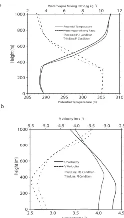
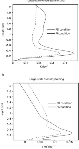
Vertical profiles of the initial specific humidity, potential temperature, and horizontal wind velocity used in the CSRM-PD and the CSRM-PI runs can be seen in Fig. 1. The vertical distribution of the time- and area-averaged large-scale forcing of temperature and humidity and the time series of surface fluxes imposed in the CSRM-PD and the

10

CSRM-PI runs are depicted in Figs. 2 and 3. The profiles of humidity and potential temperature indicate that the initial inversion layer is formed around 400 m for both the CSRM-PD run and the CSRM-PI run, respectively. Below the inversion layer,u(wind in the east-west direction) andv (wind in the north-south direction) velocities do not vary much. The plus and minus indicate eastward (northward) and westward (southward)

15

wind in theu(v) velocities. The maximum large-scale forcings are near 0.4 km for both the CSRM-PD and the CSRM-PI runs but these forcings are generally larger in the CSRM-PD than in the CSRM-PI run in the lower atmosphere below∼1 km (Fig. 2). The surface LH fluxes increase significantly in the CSRM-PD run after around 00:00 LST on 13 July while the increase is much smaller in the CSRM-PI run (Fig. 3). However,

20

the surface SH fluxes do not vary significantly throughout the simulation period for both the CSRM-PD run and the CSRM-PI run (Fig. 3).

The CSRM runs were performed in a 3-D framework. A uniform grid length of 50 m was used in the horizontal domain while the vertical grid length is uniformly 20 m below 3 km and then stretches to 480 m near the model top. Periodic boundary conditions

25

(9)

ACPD

9, 21317–21369, 2009

Title Page

Tables Figures

◭ ◮

Back Close

Full Screen / Esc

Interactive Discussion between the domain size for the CSRM runs and the size of a grid box of the GCM

runs at (30◦N, 120◦W) (whose horizontal domain length is∼100 km) is given in Sect. 5 in Lee et al. (2009a).

Aerosol number concentrations are calculated from the mass profiles using the size distributions (mode radius, standard deviation, and partitioning of mass among modes)

5

described in Chuang et al. (1997) for sulfate aerosols and Liu et al. (2005) for non-sulfate aerosols in the GCM runs. In the MBL, the background aerosol number is nearly constant and only varies vertically within 10% of its value at the surface. The time series of the vertically averaged total background aerosol number concentration in the MBL in the CSRM-PD and CSRM-PI runs is shown in Fig. 4. Generally, the aerosol

10

number varies between 200 (100) and 700 (500) cm−3for the CSRM-PD (-PI) run and is larger in the CSRM-PD run than that in the CSRM-PI run.

The treatment of aerosols within cloud follows those adopted in Lee et al. (2009a) (see Sect. 5 in Lee et al. (2009a) for details).

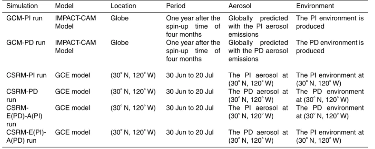
Table 1 summarizes the simulations in this study. In addition to the GCM-PD and -PI

15

runs and the CSRM-PD and -PI runs, two supplementary simulations are performed. They will be described in more detail in the following sections.

6 Results

6.1 Clear-sky case

There are differences in the parameterizations other than those used in cloud schemes

20

between the CSRM run and the GCM run (see Collins et al., 2006a; Liu et al., 2005; and Tao et al., 2003, for those differences). Hence, differences in results between the CSRM run and the GCM run may be caused not only by differences in cloud schemes but also by those in the parameterizations used for other physical and dynamical pro-cesses. Hence, comparisons between the CSRM run and the GCM run for the selected

25

(10)

ACPD

9, 21317–21369, 2009

Title Page

Tables Figures

◭ ◮

Back Close

Full Screen / Esc

Interactive Discussion Since this study focuses on the effects of different cloud parameterizations in the CSRM

run and the GCM run, it is necessary to show that the results from the comparison here are robust to different schemes other than those for cloud processes.

To show this robustness, a CSRM simulation for a clear-sky case was simulated by Lee et al. (2009a). Lee et al. (2009a) showed that the differences in the simulated

5

fields between the CSRM run and the GCM run are negligibly small for the clear-sky case. They also showed that the different radiative properties of cloud particles in the radiation schemes for the CSRM and the GCM had nearly identical responses to identical clouds. This demonstrated that differences in simulations between the CSRM run and the GCM run are mostly caused by differences in the cloud schemes. The

10

detailed description of the background philosophy used here can be found in Lee et al. (2009a).

6.2 Cloud properties and comparison with observation

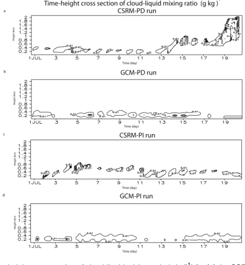
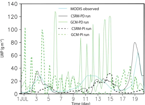
Figure 5 shows a time-height cross section of cloud-liquid mixing ratio for the GCM-PD run and -PI runs, and the CSRM-PD and -PI runs. Figure 6 shows the time series

15

of LWPs for the GCM-PD and -PI runs, and the CSRM-PD and -PI runs, smoothed over 1 day (averaged over the period between 12 h before and after a time point), and those observed by the Moderate Resolution Imaging Spectroradiometer (MODIS) on the Terra satellite, which are provided as averaged values for each day (for the 10:30 a.m. and 10:30 p.m. crossing times for July 2001 to 2008).

20

The temporal evolution of LWP in the CSRM-PD run is much closer to that observed by the MODIS than that in the GCM-PD run. LWP in the GCM-PD run generally shows much larger temporal fluctuations than the MODIS-observed LWP and the CSRM-PD-run LWP.

Figure 7 shows a time series of the effective radius of cloud liquid, conditionally

25

(11)

ACPD

9, 21317–21369, 2009

Title Page

Tables Figures

◭ ◮

Back Close

Full Screen / Esc

Interactive Discussion MODIS-observed size than the GCM-PD-run size. For the calculation of the conditional

average over cloudy regions, it is necessary to determine which grid points are in cloud. Grid points are assumed to be in cloud if the number concentration and volume-mean size of droplets is typical for clouds and fogs (1 cm−3 or more, 1 µm or more; Pruppacher and Klett, 1997). The conditional average over the grid points in cloud

5

is obtained at each time step; the conditional average is the arithmetic mean of the variable over all in-cloud grid points (grid points in clear air are excluded from the average).

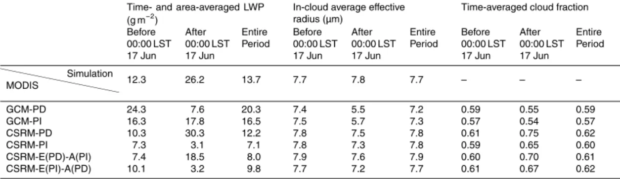
Table 2 shows the time- and domain-averaged LWP. Both the GCM and the CSRM have the larger LWPs in the PD runs than in the PI runs (over the entire simulation

10

period). However, the di_fferences in the LWP between the PD run and the PI run in the GCM differ from those in the CSRM. There is a 71% increase in LWP in the CSRM runs in the PD case compared to the PI case, while there is only a 23% increase in the LWP in the GCM runs also as shown in Fig. 8c; see the diagonal arrows for the GCM and CSRM runs in Fig. 8c, providing the diagrammatic depiction of the percentage

15

variations of LWP with simultaneously varying environment and aerosol conditions for the entire simulation period (the detailed description of Fig. 8 is given in the figure caption). Also, LWP is significantly different between the GCM-PI (-PD) run and the CSRM-PI (-PD) run; in the PD (PI) condition, the GCM has a 66 (132)% larger LWP than the CSRM.

20

Table 2 also shows the in-cloud average effective radius of droplets and the average cloud fraction. Conditional averages (over cloudy regions) at every time step were obtained for the in-cloud average e_ffective radius; only those time steps with a non-zero effective radius were included. The cloud fraction, however, was averaged over all time steps and the layer between minimum base height and maximum

cloud-25

(12)

ACPD

9, 21317–21369, 2009

Title Page

Tables Figures

◭ ◮

Back Close

Full Screen / Esc

Interactive Discussion and clouds fractions between the GCM-PI (-PD) runs and the CSRM-PI (-PD) runs

are smaller than ∼5%. Hence, the change in the cloud radiative properties is mainly controlled by the change in the LWP in the simulations. The larger LWP reflects more incident shortwave radiation, leading to smaller time- and area-averaged net downward shortwave radiation in the GCM-PI (-PD) run than in the CSRM-PI (-PD) run at the top

5

of the atmosphere; the net downward shortwave radiation is 357.5 (340.2) and 451.8 (408.4) W m−2 for the GCM-PI (-PD) run and the CSRM-PI (-PD) run, respectively. Thus, we can also see that a 2 times larger percentage variation in the change in the net downward radiation in the PD and PI runs due to the larger variation in the LWP in the CSRM runs than in the GCM runs.

10

6.3 Transition from stratocumulus to cumulus

6.3.1 LH-flux induced formation of cumulus clouds

Around 00:00 LST on 13 July, cloud depth and height start to increase in the CSRM-PD run, whereas they do not show significant changes in the CSRM-PD run, the GCM-PI run, or the CSRM-GCM-PI run (Fig. 5). The depth of the domain-averaged cloud-liquid

15

mixing ratio starts to increase substantially around 00:00 LST on 17 July and the cloud top reach∼2 km around 03:00 LST on 19 July in the CSRM-PD run (Fig. 5a). This is due to the transition of the cloud type from the stratocumulus clouds to the cumulus clouds, caused by the increase in the surface LH fluxes starting around 00:00 LST on 13 July (Fig. 3) (see Sect. 6.3 in Lee et al. (2009a) for details on the role of the surface

20

LH fluxes in the transition to cumulus clouds). This transition leads to a substantial increase in LWP in the CSRM-PD run, making LWP in the CSRM-PD run much larger than that in the CSRM-PI run after 00:00 LST on 17 July (Fig. 6 and Table 2); this is also shown in the diagonal arrow for the CSRM run in Fig. 8b, depicting the percentage variations of LWP with the simultaneously varying environment and aerosol conditions

25

(13)

ACPD

9, 21317–21369, 2009

Title Page

Tables Figures

◭ ◮

Back Close

Full Screen / Esc

Interactive Discussion diagonal arrow for the GCM run in Fig. 8b and Table 2). This is partly due to the lack of

any development of cumulus clouds in the set of GCM runs after around 00:00 LST on 17 July (Fig. 5). The development of cumulus clouds contributes to the larger increase in the time- and domain-averaged LWP over the entire simulation period in the PD run compared to that in the PI run in the CSRM than the increase in the GCM. The diagonal

5

arrows in Fig. 8a, showing the percentage variations of LWP with the simultaneously varying environment and aerosol conditions for the period before 00:00 LST on 17 July diagrammatically, indicates a smaller increase in LWP in the CSRM run than in the GCM run. However, the diagonal arrows in Fig. 8c for the entire period show a larger increase in LWP in the CSRM run due to the larger increase in LWP in the CSRM run

10

after 00:00 LST on 17 July.

The absence of cumulus clouds in the GCM-PD run is due to no explicit interac-tions between the surface LH fluxes and in-cloud buoyancy fluxes. As reported in Bretherton and Wyant (1997) and shown in Lee et al. (2009a), upward LH fluxes in the boundary layer increase with an increase in the surface LH fluxes. This increases

15

the buoyancy fluxes and turbulence levels within the cloud, creating more entrainment per unit of cloud radiative cooling. The increased entrainment leads to increasingly negative buoyancy fluxes below cloud base associated with a downward flux of warm entrained air as shown in Fig. 11b in Lee et al. (2009a). Bretherton and Wyant (1997) explained that this disrupted the mixed layer and created a weak stable layer below

20

cloud base, leading to the development of conditionally unstable cloud layer. The sta-ble layer acted as a valve that allowed only the most powerful subcloud-layer updrafts to penetrate up to the main stratocumulus cloud base, leading to the development of cumulus clouds. As the decoupling became more pronounced, the cumulus clouds developed more. Hence, the development of the conditional instability is necessary for

25

(14)

ACPD

9, 21317–21369, 2009

Title Page

Tables Figures

◭ ◮

Back Close

Full Screen / Esc

Interactive Discussion can be triggered when the large-scale moist instability (controlled by large-scale

forc-ings) exists. However, in the region of interest here (in the MBL), there is no large-scale instability developing throughout the simulation period. Hence, Hack’s scheme is not activated and thus cumulus clouds are not formed in the GCM.

6.3.2 Role of aerosols in the formation and development of cumulus clouds 5

In this section, the role of aerosols in the formation and development of cumulus clouds is examined and compared to that of the surface LH fluxes. Since aerosols are known to change the LH distribution, precipitation, and thus instability in MBL (Stevens et al., 1998), they can play a role in the transition to cumulus clouds. Two additional sim-ulations were performed for this examination. The first (second) adopts the PD (PI)

10

environment with the PI (PD) aerosol. Henceforth, the first and the second simula-tions are referred to as the CSRM-E(PD)-A(PI) run and the CSRM-E(PI)-A(PD) run, respectively (Table 1).

Due to the increase in the surface LH flux around 00:00 LST on 13 July in the PD environment, cumulus clouds start to develop in the CSRM-E(PD)-A(PI) run as in the

15

CSRM-PD run around 00:00 LST on 17 July, leading to a large increase in the averaged LWP after 00:00 LST on 17 July as shown in Table 2. However, no cumulus clouds are simulated in the CSRM-E(PI)-A(PD) run where the LH flux increase is not as signifi-cant as in the CSRM-E(PD)-A(PI) run. Since both the CSRM-E(PD)-A(PI) run and the CSRM-PD run show the formation of cumulus clouds and cumulus clouds are absent

20

in the CSRM-E(PI)-A(PD) run, we infer that the dependence of the cumulus formation on the aerosol level is very weak and the magnitude of the increase in the surface LH flux controls this formation.

Also, it is needed to be pointed out that the averaged LWP in the CSRM-E(PD)-A(PI) over the period after 00:00 LST on 17 July is∼40% smaller than that in the CSRM-PD

25

(15)

ACPD

9, 21317–21369, 2009

Title Page

Tables Figures

◭ ◮

Back Close

Full Screen / Esc

Interactive Discussion basically determined by how large the LH flux increases, the mass of cumulus clouds

is controlled by the aerosol level. Figure 11b shows that the variance of the vertical ve-locity is larger in the CSRM-PD run than in the CSRM-E(PD)-A(PI) run (after 00:00 LST on 17 July), leading to larger condensation and cloud mass after 00:00 LST on 17 July. This indicates that the interactions among the LH flux, the buoyancy flux, and

dynam-5

ics in cumulus clouds become stronger with increasing aerosols. This leads to a larger increase in the averaged LWP over the entire simulation period in the CSRM-PD run relative to the CSRM-E(PI)-A(PD) run than in the CSRM-E(PD)-A(PI) run relative to the CSRM-PI run as shown in Table 2; this is also shown in the comparison between the two vertical arrows, depicting the increasing LWP with the PI-to-PD change in the

10

environment at the PI (the left arrow) and the PD (the right arrow) aerosols, in Fig. 8c. In other words, the sensitivity of the response of the formation and development of cumulus clouds and thus the averaged LWP over the entire period to the changes in the environment (more specifically, changes in the surface LH fluxes) increases with increasing aerosols.

15

6.4 Liquid-water budget of stratocumulus clouds

A smaller time- and domain-averaged LWP is simulated in the CSRM run than in the GCM run for both the PD and the PI conditions over the entire simulation period mostly due to the smaller averaged LWP when stratocumulus clouds are a dominant cloud type in all of the GCM runs and CSRM runs before 00:00 LST on 17 July (Table 2).

20

The percentage increase in the LWP from the PI simulation to the PD simulation is also smaller in the CSRM runs than in the GCM runs in stratocumulus clouds (before 00:00 LST on 17 July); see the diagonal arrows in Fig. 8a and Table 2. Next, the analyses of the liquid-water budget terms of the CSRM runs and the GCM runs are performed to identify mechanisms which lead to different LWPs and their variation with

25

(16)

ACPD

9, 21317–21369, 2009

Title Page

Tables Figures

◭ ◮

Back Close

Full Screen / Esc

6.4.1 CSRM runs

The averaged LWPs over the period before 00:00 LST on 17 July are less than 50 g m−2 for the CSRM runs (Table 2). Hence, stratocumulus clouds here can be considered thin according to the classification of Turner et al. (2007).

To elucidate the microphysical processes controlling the LWC and thus LWP of the

5

stratocumulus clouds in the CSRM-PD run and the CSRM-PI run, the domain-averaged cumulative source (i.e., condensation) and sinks of cloud liquid were obtained. For this, the production equation for cloud liquid was integrated over the domain and over the period before 00:00 LST on 17 June for both the CSRM-PD and -PI runs. These integrations are denoted byh i:

10

hAi= 1 LxLy

Z Z Z

ρaAdxd yd zd t (1)

where Lx and Ly are the domain length (12 km), in the east-west and north-south directions, respectively. ρ_a is the air density andA represents any of the variables in this study. The budget equation for cloud liquid is as follows:

_∂q

c

∂t

=hQcondi − hQevapi − hQautoi − hQaccri (2)

15

Here,qcis the cloud-liquid mixing ratio. Qcond,Qevap,Qauto, andQaccrrefer to the rates

of condensation, evaporation, autoconversion of cloud liquid to rain, and accretion of cloud liquid by rain, respectively.

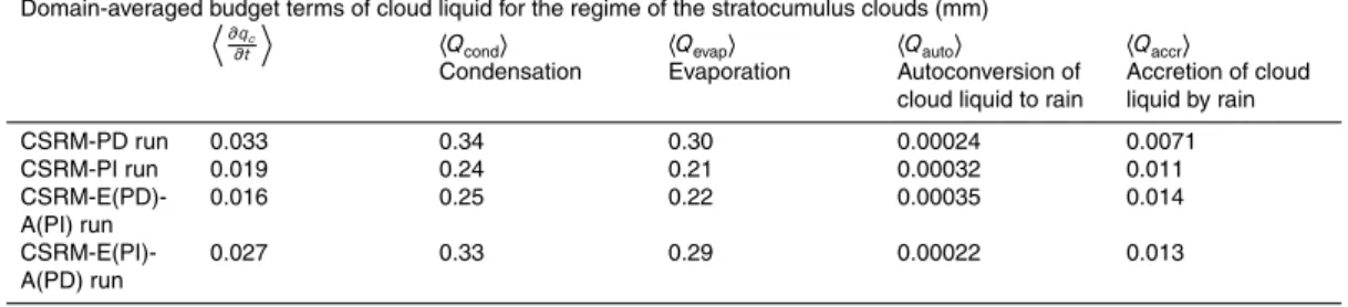
Table 3 shows the budget from Eq. (2) for the CSRM-PD run and the CSRM-PI run. The other runs in Table 3 will be discussed in the following sections. The budget results

20

(17)

ACPD

9, 21317–21369, 2009

Title Page

Tables Figures

◭ ◮

Back Close

Full Screen / Esc

Interactive Discussion The terminal fall velocity of cloud particles to which the sedimentation rate is

pro-portional increases with their increasing size. Also, the sedimentation of cloud mass is mainly controlled by the sedimentation of cloud particles larger than the critical size for collection around∼20–∼40 µm in radius (Pruppacher and Klett, 1997). Autoconversion and accretion are processes that control the growth of cloud particles after they reach

5

this critical size or larger (Rogers and Yau, 1989). Hence, the small contribution of au-toconversion and accretion to the LWC implies that the role of sedimentation of cloud particles in the determination of LWC is not as significant as that of condensation and evaporation.

Also, there are much larger differences in condensation and evaporation as

com-10

pared to those in autoconversion and accretion between the CSRM-PD run and the CSRM-PI run (Table 3). This implies that the variation of sedimentation (associated with that of autoconversion and accretion) is much smaller than that of condensation and evaporation due to the change from the PI condition to the PD condition.

Figure 9a and b shows the time- and domain-averaged vertical distribution of

con-15

densation and cloud-mass changes due to sedimentation for the CSRM-PD run and the CSRM-PI run during the time period when stratocumulus clouds dominate. Cloud mass here is the sum of the mass of all species associated with warm microphysics, i.e., cloud liquid and rain. The magnitude of the condensation rate is substantially larger than that of the sedimentation-induced cloud-mass changes for both of the CSRM-PD

20

run and the CSRM-PI run. Also, the magnitude of difference in the condensation rate between the CSRM-PD run and the CSRM-PI run is substantially larger than that in sedimentation-induced mass changes. Hence, as implied by the budget analysis, LWC and LWP and their responses to the change from PI to PD conditions are strongly controlled by condensation while the role of sedimentation in their determination is

25

negligible.

(18)

ACPD

9, 21317–21369, 2009

Title Page

Tables Figures

◭ ◮

Back Close

Full Screen / Esc

6.4.2 Interactions among CDNC, condensation, and dynamics

The equation for the change in mass of droplets from vapor diffusion as used in this study, integrated over the size distribution, is:

d m

d t =Nd4πψFReSρvsh (3)

where N_d is the CDNC, ψ the vapor diffusivity, and ρvsh the saturation water vapor

5

mixing ratio. S is the supersaturation, given by ρva ρ_vsh−1

where ρva is water vapor

mixing ratio. FRe is the integrated product of the ventilation coefficient and droplet

diameter which is given by

FRe =

∞

Z

0

DfRefgam(D)d D (4)

where D is the diameter of the droplets, fRe the ventilation coefficient, and fgam(D)

10

the size distribution function, given by _Γ1₍_υ₎_DD

n

ν−1

1

D_n exp

−_DD

n

. fRe is given by

1.0+0.229vtD

Vk

0.5

ηwherev_tis the terminal velocity andV_k the kinematic viscosity

of air andηthe shape parameter (Cotton et al., 1982).

Among the variables associated with the condensational growth of droplets in Eq. (3), differences in the supersaturation and CDNC contribute most to the differences in

con-15

densation between the CSRM-PD run and the CSRM-PI run. Percentage differences in the other variables are found to be∼two orders of magnitude smaller than those in su-persaturation and CDNC throughout the simulations. Figure 10a shows the time series of CDNC and Fig. 10b shows the time series of supersaturation when the stratocu-mulus clouds dominate in both of the simulations, conditionally averaged over areas

20

(19)

ACPD

9, 21317–21369, 2009

Title Page

Tables Figures

◭ ◮

Back Close

Full Screen / Esc

Interactive Discussion condensation rate>0 (grid points with no condensation are excluded from the average).

Figure 10a and b indicates that supersaturation is generally larger in the CSRM-PI run than in the CSRM-PD run. However, the condensation rate is generally higher, leading to larger cumulative condensation in the CSRM-PD run than in the CSRM-PI run during the time when stratocumulus clouds dominate (Table 3). This is ascribed to the larger

5

CDNC (as shown in Fig. 10a) (mainly due to the increased aerosols in the CSRM-PD run) providing a larger surface area for water-vapor condensation in the CSRM-PD run compared to that in the CSRM-PI run. The e_ffects of the CDNC increase on the surface area of droplets and thus on condensation compete with the effects of the su-persaturation decrease on the condensation. The effects of the increased surface area

10

for condensation outweigh the e_ffects of decreased supersaturation, leading to an in-crease in the condensation in the CSRM-PD run. This leads to the larger averaged LWP over the period prior to 00:00 LST on 17 June in the CSRM-PD run compared to that in the CSRM-PI run.

Increased condensation provides more condensational heating, and, thereby,

inten-15

sifies updrafts as shown in Fig. 11a which depicts the vertical distribution of the time-and domain-averaged variance of the vertical velocity for the CSRM-PD run time-and the CSRM-PI run prior to 00:00 LST on 17 June; the variance of the other experiments in Fig. 11a will be discussed in the following sections. The increased updrafts in turn increase condensation, establishing a positive feedback between updrafts and

con-20

densation, and playing a crucial role in the increased LWP in the CSRM-PD run. Note that increased condensation not only increases evaporation, and thus, entrainment, but also increases LWC. The effects of condensation on LWC outweigh those of evap-oration and entrainment, leading to the increased LWP in the PD run. Hence, the interactions among CDNC, condensation, and dynamics (i.e., updrafts) mostly

deter-25

(20)

ACPD

9, 21317–21369, 2009

Title Page

Tables Figures

◭ ◮

Back Close

Full Screen / Esc

6.4.3 Effects of cloud-base instability on LWP

The surface precipitation is absent in the CSRM runs before 00:00 LST on 17 July dur-ing the time when stratocumulus clouds dominate as indicated by Fig. 9b. As shown by Jiang et al. (2002) and Lee et al. (2009a, b), when precipitating particles evapo-rate completely before reaching the surface, even the slightly increased evaporation

5

of precipitation around the cloud base can cause increased instability concentrated around the cloud base (which leads to increased updrafts and condensation) in strati-form clouds.

Figure 12a depicts the domain-averaged rain evaporation in the CSRM-PD run and the CSRM-PI run; the results of CSRM-E(PD)-A(PI) experiment in Fig. 12 will be

de-10

scribed in the following sections. The figure confirms that the precipitation does not reach the surface and that rain evaporates mostly around cloud base (atz/z_t∼0.4 to 0.5 wherezt is cloud-top height) in both the CSRM-PD run and the CSRM-PI run. As shown in Fig. 12b, which depicts the vertical profile of the time- and area-averaged rate of conversion of cloud liquid to rain, more droplets are converted to rain in the CSRM-PI

15

run. Hence, more rain falls to around the cloud base in the CSRM-PI run than in the CSRM-PD run. This in turn leads to a larger evaporation of rain just below the cloud base as shown in Fig. 12a. Figure 12c, which depicts area-averaged profile of lapse rate d θ_{d z} over 16:00 LST on 30 June–00:00 LST on 17 July, shows that the increase in evaporation below cloud base leads to a larger instability in the CSRM-PI run (d θ_{d z} is

20

smaller in the CSRM-PI run below cloud base). Here,θis potential temperature. Fig-ure 12d shows the domain-averaged profile of potential temperatFig-ure over 16:00 LST on 30 June–00:00 LST on 17 July. Smaller d θ_{d z} below cloud base leads to lower potential temperature in the CSRM-PI run around cloud base.

The increased cloud-base instability tends to increase condensation in the CSRM-PI

25

(21)

ACPD

9, 21317–21369, 2009

Title Page

Tables Figures

◭ ◮

Back Close

Full Screen / Esc

Interactive Discussion the larger time- and domain-averaged updrafts, condensation and thus LWP in the

CSRM-PD run during the time when stratocumulus clouds dominate.

6.4.4 Effects of environmental conditions on LWP

There are differences in both the background aerosols and environmental conditions (characterized by the initial condition, large-scale forcings, and surface fluxes) imposed

5

on the CSRM between the CSRM-PD run and the CSRM-PI run. It is well known that environmental conditions affect aerosol-cloud interactions (Jiang et al., 2002; Acker-man et al., 2004; Guo et al., 2007). Hence, it is needed to examine the relative role of changes in aerosols in determining the LWP response to the PI-to-PD change in thin stratocumulus clouds (explained in the previous section) to that of changes in

environ-10

mental conditions.

The budget equation for cloud liquid water mass (Eq. 2) for the time period dur-ing which stratocumulus clouds dominate for both the PD run and the CSRM-E(PD)-A(PI) run before 00:00 LST on 17 July, is shown in Table 3. As was the case in the comparison between the CSRM-PD run and the CSRM-PI run, condensation

con-15

trols the variation of the liquid-water budget between the PD run and the CSRM-E(PD)-A(PI) run, while the role of the conversion of liquid water to precipitation (i.e., autoconversion₊accretion) in the variation is negligible. As shown in Fig. 12c, a larger cloud-base instability develops in the CSRM-E(PD)-A(PI) run than in the CSRM-PD run; no surface precipitation is simulated during the time period when stratocumulus

20

clouds dominate in the CSRM-E(PD)-A(PI). The lower aerosol concentration leads to more conversion of cloud liquid to rain and thus more cloud-base rain evaporation to induce a larger cloud-base instability in the E(PD)-A(PI) run than in the CSRM-PD run (Fig. 12). However, the larger instability does not lead to the larger updrafts, condensation, and LWP in the CSRM-E(PD)-A(PI) run than in the CSRM-PD run when

25

(22)

ACPD

9, 21317–21369, 2009

Title Page

Tables Figures

◭ ◮

Back Close

Full Screen / Esc

Interactive Discussion the increased aerosols on CDNC and thus condensation outweigh the effects of the

increased cloud-base instability as also shown in the comparison between the CSRM-PD run and the CSRM-PI run. Hence, the mechanisms elaborated in the previous sections leading to larger LWP in the CSRM-PD run (when stratocumulus clouds are dominant) are operative with the change in aerosols regardless of whether the change

5

in the environmental conditions occurs. This is supported by the comparison between the CSRM-PI run and the CSRM-E(PI)-A(PD) run for the period before 00:00 LST on 17 July. The CSRM-E(PI)-A(PD) run with higher aerosols than those in the CSRM-PI run has higher condensation (controlling the cloud-mass and thus LWP responses to aerosols), leading to larger updrafts, LWC, and thus LWP in the CSRM-E(PI)-A(PD) run

10

(Fig. 11a, Tables 2 and 3); this can also be seen in lower horizontal arrow, depicting increasing LWP with the PI-to-PD change in aerosols at the PI environment, in Fig. 8a. Although Fig. 11a shows updrafts averaged over 16:00 LST on 30 June–00:00 LST on 17 July, the larger averaged updrafts in the E(PI)-A(PD) run than in the CSRM-PI run also holds over the entire simulation period. This is despite the lower cloud-base

15

instability in the CSRM-E(PI)-A(PD) run than that in the CSRM-PI run; due to the in-creased surface areas of droplets, condensation increases in the CSRM-E(PI)-A(PD).

The LWP variations due to the change from the PI environmental condition to the PD environmental condition for both the PI aerosol and the PD aerosol is one to two orders of magnitude smaller than the LWP variation shown between the CSRM-PD

20

run and the CSRM-PI run before 00:00 LST on 17 June (Table 2). This can be seen in the LWPs in Table 2 for the CSRM-PI (the CSRM-PD) run and the CSRM-E(PD)-A(PI) (the CSRM-E(PI)-A(PD)) run compared to that between the CSRM-PI run and the CSRM-PD run for the PI (PD) aerosol. This can also be seen in the comparison of a diagonal arrow to a vertical arrow either at the PD aerosol (the right vertical arrow)

25

(23)

ACPD

9, 21317–21369, 2009

Title Page

Tables Figures

◭ ◮

Back Close

Full Screen / Esc

Interactive Discussion This can be seen in the LWP variation in Table 2 between the PI (the

CSRM-PD) run and the CSRM-E(PI)-A(CSRM-PD) (the CSRM-E(CSRM-PD)-A(PI)) run compared to that between the CSRM-PI run and the CSRM-PD run for the PI (PD) environment. This can also be seen in the comparison of a diagonal arrow to a horizontal arrow either at the PD environment (the upper horizontal arrow) or at the PI environment (the lower

5

horizontal arrow) for the CSRM runs in Fig. 8a. This indicates that the aerosol changes play a much more important role in the LWP changes (associated with the PI-to-PD transition) than the changes in the environment for stratocumulus clouds.

Also, it should be pointed out that there is an increase in condensation and thus LWP due to the change from the PI environmental condition to the PD environmental

10

condition for each of the PI and the PD aerosols when stratocumulus clouds domi-nate, though the increase is negligibly small (Tables 2 and 3); also, see a vertical arrow showing increasing LWP with the PI-to-PD change in the environment either at the PD aerosol (the right arrow) or at the PI aerosol (the left arrow) for the CSRM run in Fig. 8a. This is associated with the surface LH flux before the development of the

15

cumulus clouds which is generally larger in the PD environment than in the PI envi-ronment (Fig. 3). As Guo et al. (2007) showed, the increase in the surface LH flux leads to increases in the LWP of stratocumulus clouds. The larger surface LH fluxes induce larger buoyancy fluxes. This in turn induces a larger intensity of vertical ve-locity, leading to larger condensation and LWP in thin stratocumulus clouds in the PD

20

environment compared to the PI environment for the given aerosols (Figs. 11a and 8a and Tables 2 and 3). Also, as can be seen in Fig. 2, showing the vertical distribution of the time- and area-averaged large-scale forcings of the temperature and humidity in the PD environment and the PI environment, there is a larger large-scale advection of humidity and temperature in the PD environment in the MBL (generally below∼1 km

25

(24)

ACPD

9, 21317–21369, 2009

Title Page

Tables Figures

◭ ◮

Back Close

Full Screen / Esc

6.4.5 GCM runs

The CSRM is able to simulate the condensation variation not only from the large-scale environment but also from cloud-scale motions by resolving the cloud-scale interac-tions among aerosols, CDNC, supersaturation, and updrafts. However, the saturation adjustment in the GCM with no consideration of the effect of varying surface area of

5

droplets on condensation is strongly controlled by the large-scale environment which is resolvable in the GCM. The variation of large-scale environment is not substantial, leading to ∼1.5 times smaller percentage increase of condensation in the GCM-PD run than in the CSRM-PD run with the PI-to-PD change as seen in Fig. 9a and c. As shown in the previous section, even in the CSRM runs, when the e_ffect of aerosols on

10

condensation is excluded and only that of environment is included, the LWP variation with the PI-to-PD change decreases substantially as compared to when both effects are included.

Figure 9c and d shows that the variation in the conversion of cloud liquid to rain (i.e., autoconversion+collection) between the PI and PD conditions accounts for ∼50% of

15

the variation of condensation between the GCM-PD run and the GCM-PI run, while the variation in this conversion accounts for only∼0.0001% of the variation of condensation between the CSRM-PD run and the CSRM-PI run. Due to this larger decrease in conversion, the GCM-PD run shows a larger percentage increase (49%) in the LWP than that in the CSRM-PD run (41%) (see the diagonal arrows in Fig. 8a) despite the

20

smaller increase in condensation between the PI run and the PD run before 00:00 LST on 17 June when stratocumulus clouds dominate for the GCM-PD, -PI, CSRM-PD, and -PI runs.

Also, similar to the LWP change between the GCM-PD run and the GCM-PI run, for both the GCM-PD and GCM-PI runs, the conversion of cloud liquid to rain plays just as

25

(25)

ACPD

9, 21317–21369, 2009

Title Page

Tables Figures

◭ ◮

Back Close

Full Screen / Esc

Interactive Discussion CSRM than the diagnosed supersaturation in the GCM in each of the PI run and the

PD run. This leads to increased condensation in the GCM-PD (-PI) run as compared to that in the CSRM-PD (-PI) run. This increased condensation is large enough to re-sult in a larger LWP despite the higher conversion efficiency (i.e., the ratio between the conversion of cloud liquid to rain and condensation) in the GCM-PD (-PI) run than in

5

the CSRM-PD (-PI) run during the time when stratocumulus clouds dominate.

Small cloud droplets grow to a critical size for (active) collection not only by the tur-bulent collisions among them but also by condensation; for particles smaller than the critical size, condensational growth is as important as the growth through the turbulent collisions and particles grow via positive feedbacks between the condensational growth

10

and the growth through these turbulent collisions, though, above the critical size, the growth through collection is dominant (Rogers and Yau, 1991). Thus, it is likely that, as clouds get thinner, these feedbacks get weaker and thus the conversion efficiency gets lower, since condensation in thinner clouds with lower LWP is likely to be lower. Hence, for the thin stratocumulus clouds simulated here, the conversion of droplets to

15

rain (here, defined as particles whose radius is larger than 40 µm) is inactive enough to result in nearly inactive sedimentation as compared to condensation. Also, Khairoutdi-nov and Kogan (2000) indicated that the sensitivity of the conversion of cloud liquid to rain to varying CDNC was weaker at low LWC than at high LWC based on results from a bin model taking into account the feedbacks between condensation and collisions.

20

This implies that the sensitivity of sedimentation to aerosol changes (leading to CDNC changes) is also weaker at low LWC. The variation of the conversion of cloud droplets to rain with varying aerosols (as shown in the comparison between the CSRM-PD run and the CSRM-E(PD)-A(PI) run and between the CSRM-PI run and the CSRM-E(PI)-A(PD) run) is not large enough to make a significant difference in the sedimentation of

25

(26)

ACPD

9, 21317–21369, 2009

Title Page

Tables Figures

◭ ◮

Back Close

Full Screen / Esc

Interactive Discussion by predicting supersaturation and CDNC and considering the spectral information in

the collection processes. Hence, they are able to produce results fairly consistent with the implications of the theoretical consideration about the role of the conversion and sedimentation in the LWP determination in thin clouds and the previous study about the dependence of the response of the role to aerosols on LWP. However, the

satura-5

tion adjustment scheme and the autoconversion and collection parameterizations with a fixed threshold and a constant collection efficiency in the GCM runs are not able to take into account the feedbacks explicitly. The results here demonstrate that the ab-sence of the feedbacks leads to much more efficient conversion of cloud liquid to rain and much more important role of the conversion in the cloud response to aerosols.

10

6.5 Dependence of the LWP responses to aerosols on cloud type

It is notable that there are larger increases in the averaged LWP over the period involv-ing cumulus clouds with the change from the PI aerosols to the PD aerosols than in the period when stratocumulus clouds are dominant (i.e., comparing the CSRM-PD run and the CSRM-E(PD)-A(PI) run). This is shown in the comparison between the upper

15

horizontal arrows in Fig. 8a and b. The upper horizontal arrow in Fig. 8b, representing the LWP change with the PI-to-PD change in aerosols at the PD environment for the period when cumulus clouds form, shows larger LWP variation than that in Fig. 8a, representing the same as the upper horizontal arrow in Fig. 8b but for the period when stratocumulus clouds dominate. These increases in the period with cumulus clouds

20

are also larger than those between the CSRM-PI run and the CSRM-E(PI)-A(PD) run for the simulation period when stratocumulus clouds dominate either before or after 00:00 LST on 17 July (see Table 2); note that stratiform clouds dominate for the entire simulation period with the PI environment. This can also be seen in the comparison of the lower horizontal arrow in each of Fig. 8a and b to the upper arrow in Fig. 8b;

25

(27)

ACPD

9, 21317–21369, 2009

Title Page

Tables Figures

◭ ◮

Back Close

Full Screen / Esc

Interactive Discussion cloud type and aerosol effects on cumulus clouds induce larger changes in cloud mass

than those on stratiform clouds.

7 Summary and conclusion

A 20-day simulation was performed using a CSRM coupled with a double-moment microphysics for a case of thin stratocumulus clouds located at (30◦N, 120◦W) offthe

5

coast of the western Mexico for each of the PD condition (the CSRM-PD run) and PI condition (the CSRM-PI run). Initial conditions, large-scale forcings, surface fluxes, and aerosols produced by a GCM simulation with the PD (PI) conditions (the GCM-PD (PI) run) at (30◦N, 120◦W) were imposed on the CSRM-PD (PI) run. This enabled a comparison of the responses of thin clouds to the transition from the PI condition to

10

the PD condition simulated in a GCM to those in the CSRM. The much higher resolution and more detailed representation of cloud microphysics were used for the CSRM as compared to those in the GCM, enabling the CSRM to act as a benchmark to assess these responses simulated by the GCM.

Zhang et al. (2003) stated that two lines of complication arose in the parameterization

15

of clouds in GCMs. The first is from the spatial and temporal subgrid-scale variability of the dynamic, thermodynamic, and hydrological variables within a GCM grid box. Most GCMs (including the GCM used here) have relied on highly simplified parameteriza-tions of subgrid-scale variables due to the use of coarse resoluparameteriza-tions. The second is from microphysical processes associated with aerosols (acting as cloud condensation

20

nuclei (CCN) or ice nuclei (IN)) and hydrometeors.

This study indicates that the first line of complication (discussed in Zhang et al., 2003), which is the reliance on the parameterization of subgrid-scale variables with no explicit simulation of these variables, can lead to substantial errors in the evaluation of the changing cloud properties since industrialization; the subgrid-scale interactions

25

(28)

ex-ACPD

9, 21317–21369, 2009

Title Page

Tables Figures

◭ ◮

Back Close

Full Screen / Esc

Interactive Discussion plicit simulation of these interactions prevented the formation of cumulus clouds in the

GCM. The development of cumulus clouds in the CSRM led to substantial di_fferences between the GCM and CSRM in the response of the LWP and thus radiation to the change from PI to PD conditions.

Also, the coarse spatial resolution (a main cause of the first line of complication

5

discussed in Zhang et al., 2003) employed in climate models is not able to resolve the effect of aerosols on interactions among supersaturation, the surface area of cloud particles (associated with CDNC), condensation, and updrafts in the cloud layer and the instability around cloud base, which play important roles in aerosol effects on LWP in the thin stratocumulus clouds simulated by the CSRM here. So far, in general,

10

parameterizations for the representation of the LWP variation with aerosols have simply relied on changes in the autoconversion of cloud liquid and the change in sedimentation of cloud liquid and rain with varying aerosols in climate models including the GCM used in this study. They do not take into account feedbacks among microphysics, dynamics, and the instability which are affected by aerosols.

15

In addition, this study indicates the second line of complication discussed in Zhang et al. (2003) can also cause a high uncertainty in the simulation of changing cloud prop-erties since industrialization. Most of GCMs (including the GCM used here) and some of CSRMs have adopted saturation adjustment schemes which are not able to predict supersaturation and thereby to consider the effects of interactions between

supersatu-20

ration and the surface area of cloud particles (varying with aerosols) on condensation. This implies that although the first line of complication were removed by using high resolutions, the effect of aerosols on these interactions would not be simulated when the saturation adjustment is used in climate models. When the stratocumulus clouds dominate, the increase in the LWP between the PD and PI runs was controlled by the

25

(29)

ACPD

9, 21317–21369, 2009

Title Page

Tables Figures

◭ ◮

Back Close

Full Screen / Esc

Interactive Discussion the spectral information, the decrease in the conversion of cloud liquid to rain played

a role that was as important as that of the increase in condensation with the PI to PD change. This contributed to the large differences in the response of the LWP to the change from the PI condition to the PD condition between the GCM and the CSRM simulations here.

5

The first and second lines of complications also led to substantial discrepancies be-tween the CSRM and the GCM for both PI and PD conditions. In both the CSRM-PD run and the CSRM-PI run, the interactions between CDNC and supersaturation play an important role in the determination of condensation and LWP, in addition to the in-teractions around the cloud base. Supersaturation produced by updrafts is consumed

10

by the condensation of water vapor onto droplets and increasing (decreasing) CDNC provides increasing (decreasing) surface areas of droplets for condensation, leading to decreasing (increasing) equilibrium supersaturation, for a given background aerosol level. These interactions are explicitly simulated in the CSRM runs due to the use of the high resolution and the prediction of supersaturation while condensation is

di-15

agnosed based on environmental conditions in the GCM runs. It is found that the explicit simulation of these interactions (between CDNC and supersaturation and be-tween rain evaporation and cloud-base instability) tends to produce less condensation in the CSRM run as compared to the saturation adjustment scheme in the GCM run in the stratocumulus regime in both the PD and the PI runs. Also, these interactions lead

20

to the smaller LWP being closer to the MODIS-observed LWP in the CSRM-run than in the GCM-run in the stratocumulus regime. Hence, for these aerosol and environmen-tal conditions, climate models with the simplified conversion schemes and saturation adjustment are likely to overestimate the mass of stratocumulus clouds.

This study demonstrates a large uncertainty (from the first and second lines of

com-25

(30)

ACPD

9, 21317–21369, 2009

Title Page

Tables Figures

◭ ◮

Back Close

Full Screen / Esc

Interactive Discussion Turner et al., 2007; McFarlane and Evans, 2004; Shupe and Interieri, 2004; Marchand

et al., 2003). Therefore, microphysics parameterizations, able to predict particle mass and number, and thereby, surface area, coupled with a prediction of supersaturation, need to be implemented into climate models for a correct assessment of the effects of aerosols on thin clouds. These parameterizations should also be able to take into

5

account the interactions between rain evaporation and the cloud-base instability. The transition of the cloud type from stratocumulus to cumulus due to the increasing magnitude of the LH-flux increase implies that the climate change associated with the increasing greenhouse gases and thus the surface temperature can act in favor of creasing the frequency of the stratocumulus-to-cumulus transition. This is because

in-10

creases in temperature near the Earth’s surface due to increases in greenhouse gases can increase the surface LH fluxes as indicated by Bretherton and Wyant (1997) who showed that the surface LH fluxes increase with the increasing sea surface temper-atures. This may have impacts on the transition of stratocumulus clouds to cumulus clouds and thus on the mass of warm clouds, in turn affecting the effects of warm clouds

15

on the global radiation budget. It should be pointed out that supplementary simulations indicated that the increase of aerosols since industrialization can increase the sensitiv-ity of the stratocumulus-to-cumulus transition and the associated changes in the mass of warm clouds to increasing LH fluxes (associated with the greenhouse gases). Also, supplementary simulations demonstrated that aerosol e_ffects on clouds depend on the

20

cloud type; the mass of water in cumulus clouds is more sensitive to aerosols than the mass of water in stratocumulus clouds. Hence, the more frequent development of warm cumulus clouds due to increasing LH fluxes associated with the increasing greenhouse gases is likely to increase the sensitivity of the mass of warm clouds to aerosols. As shown in this study, the GCM is not able to simulate this

deepening-25