www.ann-geophys.net/25/1025/2007/
© European Geosciences Union 2007
Geophysicae
Global and local disturbances in the magnetotail during
reconnection
T. V. Laitinen1, R. Nakamura2, A. Runov2, H. Rème3, and E. A. Lucek4
1Finnish Meteorological Institute, Space Research, PL 503, 00101 Helsinki, Finland 2Space Research Institute, Austrian Academy of Sciences, 8042 Graz, Austria 3Centre d’Etude Spatiale des Rayonnements, Toulouse, France
4The Blackett Laboratory, Imperial College, London, UK
Received: 11 December 2006 – Revised: 13 March 2007 – Accepted: 13 April 2007 – Published: 8 May 2007
Abstract. We examine Cluster observations of a reconnec-tion event atxGSM=−15.7REin the magnetotail on 11 Oc-tober 2001, when Cluster recorded the current sheet for an extended period including the entire duration of the recon-nection event. The onset of reconrecon-nection is associated with a sudden orientation change of the ambient magnetic field, which is also observed simultaneously by Goes-8 at geosta-tionary orbit. Current sheet oscillations are observed both before reconnection and during it. The speed of the flapping motions is found to increase when the current sheet under-goes the transition from quiet to active state, as suggested by an earlier statistical result and now confirmed within one sin-gle event. Within the diffusion region both the tailward and earthward parts of the quadrupolar magnetic Hall structure are recorded as an x-line passes Cluster. We report the first observations of the Hall structure conforming to the kinks in the current sheet. This results in relatively strong fluctuations inBz, which are shown to be the Hall signature tilted in the yzplane with the current sheet.
Keywords. Magnetospheric physics (Magnetospheric con-figuration and dynamics; Magnetotail) – Space plasma physics (Magnetic reconnection)
1 Introduction
The magnetotail is a natural laboratory for magnetic recon-nection. The antiparallel lobe fields set up the stage for the simplest possible reconnection geometry; however, the re-connection process need not choose the most simple form of a large-scale two-dimensional x-line, and many observations indicate that it indeed does not. To name some examples, there are reports on off-centre and bifurcated current sheet profiles (Hoshino et al., 1996; Asano et al., 2003; Runov
Correspondence to:T. V. Laitinen
et al., 2005; Thompson et al., 2006), current sheet flapping motion (Lui et al., 1978; Sergeev et al., 2003, 2004), mul-tiple x-lines (Deng et al., 2004; Eastwood et al., 2005), and bursty bulk flows (Baumjohann et al., 1990) that can be inter-preted as signs of localized reconnection events (Shay et al., 2003) or transient reconnection events (Sergeev et al., 1987). From the global point of view reconnection is an impor-tant piece in the puzzle of magnetospheric dynamics. Tail reconnection is recognized as the main energy source of sub-storms (Baker et al., 1996): The substorm sequence com-mences with a growth phase, during which magnetic flux is added to the tail and the near-Earth current sheet grows thinner. At substorm onset a neutral line forms in the tail, most frequently at a radial distance of 20–30RE but some-times also closer to the Earth (Nagai, 2006, and references therein). Global MHD simulations support the view that the reconnection site acts as a centre of Poynting flux focussing, where the incoming electromagnetic energy is partly con-verted to kinetic and thermal energy of the plasma and where some of it is diverted earthward (Laitinen et al., 2005). How-ever, debate continues on whether tail reconnection should be regarded more as a “primus motor" or as a mediator and whether the energy it releases comes from the energy storage of the tail or as non-delayed Poynting flux from the magne-topause (Pulkkinen et al., 2006).
x
y
Cluster
Goes-8
10.5
2.3
-6.2
-15.7
−1000 0 1000 −1000
0 1000
1 2
3 4
∆ X (km)
∆
Y (km)
−1000 0 1000 1 2
3 4
∆ X (km)
∆
Z (km)
−1000 0 1000
1 2
3 4
∆ Y (km)
∆
Z (km)
(b)
Fig. 1. (a) Cluster and Goes-8 satellites in the magnetosphere
at 03:30 UT on 11 October 2001. In GSM coordinates their
locations were: Cluster at [−15.7,10.5,2.5]RE and Goes-8 at
[−6.2,2.3,−0.7]RE. The magnetopause drawn is a sketch only.
Earth and the satellites are not to scale. (b)The relative locations
of the four Cluster spacecraft. Cluster 1 is black, C2 red, C3 green and C4 blue. The figures are centered at the barycentre of the tetra-hedron.
In this article we examine Cluster observations of an event which on the first glimpse appears as a classic example of a tailward-retreating x-line, but on closer examination shows several intriguing features: In Sect. 2 we introduce the event and show that a large-scale orientation change of the ambi-ent magnetic field takes place when the reconnection starts. In the Discussion (Sect. 5) we suggest that this may reflect a global change in the magnetotail geometry. In Sect. 3 we find an x-line from the tailward edge of the diffusion region; some possible explanations to this asymmetry are also given in the Discussion. The event also includes strong flapping motion of the current sheet and rapid fluctuations in the y-and z-components of the magnetic field. Cluster was fortu-nate enough to record the current sheet for a long period in-cluding the whole duration of the reconnection event, which allows us to compare the flapping motions at the same place
during quiet and active times. This is described in Sect. 4; in addition, we show that the Hall fields conform to the kinks in the current sheet, which explains at least some of the largest reversals inBzwithin the diffusion region.
2 Large-scale features
2.1 An overview of the event
We examine the interval 03:00–04:00 UT on 11 October 2001, when Cluster observed a flow reversal and several cur-rent sheet crossings in the duskside flank of the magneto-sphere. Several other ground-based and geostationary in-struments recorded signatures of moderate activity. We will show that the reconnection onset occurred approximately at 03:25 UT; at that time the Cluster tetrahedron was located at[x, y, z]=[−15.7,10.5,2.5]REin GSM coordinates. The positions of the spacecraft are shown in Fig. 1. Data from the Cluster magnetic field instrument FGM (Balogh et al., 2001) and ion spectrometer CIS (Rème et al., 2001) are used in this study.
Panels (a–d) in Fig. 2 show the solar wind conditions dur-ing the event period and durdur-ing the preceddur-ing hour. The data are from the ACE spacecraft at the L1 libration point, but they have been time-shifted by 65 min. The plots thus show the time evolution of the parameters at Earth assuming that the solar wind propagated unchanged from L1 at a speed of 380 km/s. This approximation is reasonable because the so-lar wind was quite steady during the period (panels b and c). The moderate velocity and density combine to a relatively small dynamic pressure of about 1 nPa (panel d). The mag-netic field (panel a) had an almost constant magnitude of 5 nT during the entire period and was directed duskward most of the time. Its z-component fluctuated around zero. Therefore the reconnection event was not preceded by enhanced energy loading into the magnetosphere. This is confirmed by the ground magnetometer (panel e) and geostationary energetic electron (f) data, which do not show any sign of a substorm growth phase preceding the reconnection onset time.
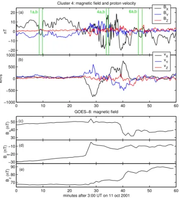
Figure 3 shows the magnetic field and proton velocity components measured by Cluster 4 from 03:00 to 04:00 UT. An eye-catching signature of reconnection are the two fast plasma flows, first tailward at 03:25–03:31 and then earth-ward at 03:36–03:43. Proton distribution functions (not shown) confirm that during the periods of fastest flow (03:28–03:30 and 03:39–03:41, when|v|exceeds 700 km/s), the velocity moments reflect well collimated bulk flows. The flow reversal suggests that this is a classic example of an x-line that moves tailward past the spacecraft.
−5 0 5 nT Bx By Bz −50 0 50 km/s vy vz −400 −350 km/s 0.5 1 1.5 nPa −300 −200 −100 0 ∆ BX [nT] PBQ GILL FCHU
2 2:15 2:30 2:45 3 3:15 3:30 3:45 4 102
104 106
differential flux
Hours on 11 October 2001 Solar wind data is time−shifted
vx
sw dynamic pressure
(a)
(b)
(c)
(d)
(e)
(f)
Fig. 2. (a–d)Solar wind conditions at 02:00–04:00 UT on 11 October 2001: components of the interplanetary magnetic field and solar wind velocity in GSM coordinates, and solar wind
dy-namic pressure. (e) Change in the northward (X) component
of the magnetic field at three Canadian magnetometer stations: Poste de la Baleine (PBQ), Gillam (GILL) and Fort Churchill
(FCHU). (f) LANL geosynchronous electron data: differential
flux (cm−2s−1sr−1keV−1) of electrons recorded by the
geosyn-chronous satellite 1990-095, which passed midnight meridian at 02:20 UT. The energy ranges of the curves are, from top to bottom: 50–75 keV, 75–105 keV, 105–150 keV, 150–225 keV, 225–315 keV and 315–500 keV.
Similar time-ordering unfortunately cannot be used in the present event. There is no distinguished majorBz reversal, and the time-ordering of flow reversal at different satellites cannot be established, most likely because the spatial scale of the flow reversal region is much larger than the separation of the spacecraft. However, considering the lack of observa-tion of other outflow jets than the two even though Cluster stays in the current sheet, and the clear Hall signature at the observed flow reversal (discussed in Sect. 3), the scenario of a tailward moving x-line is best consistent with the observa-tions.
From theBxcomponent it is seen that Cluster reached the centre of the current sheet already before the start of the re-connection event, experienced several crossings during the
−20 −10 0 10 20 nT
Cluster 4: magnetic field and proton velocity
BX BY BZ
0 10 20 30 40 50 60
−1000 −500 0 500 1000 km/s vX vY v Z 30 40 50 Bx (nT)
GOES−8: magnetic field
−30 −20 −10
By
(nT)
0 10 20 30 40 50 60
70 80 90
Bz
(nT)
minutes after 3:00 UT on 11 oct 2001
1a,b 4a,b 6a,b
(a)
(b)
(c)
(d)
(e)
Fig. 3.Upper part: the components of magnetic field and proton ve-locity measured by Cluster 4, 03:00–04:00 UT on 11 October 2001, in GSM coordinates; magnetic field from FGM and proton veloc-ity from CIS-CODIF. Lower part: the magnetic field components measured by Goes-8 during the same interval.
event and remained within the current sheet even after it. The start of the tailward flow and the end of the earthward flow can be therefore interpreted as the start and end of reconnec-tion – in this sector of the tail – and not just the satellites moving into or away from the current sheet. Thus, the obser-vation suggests that the duration of the reconnection event was about 18 min. In addition, there are some current sheet crossings both before and after the reconnection event. Bz is weak but positive before the event, which probably means that the reconnection started on closed field lines.
The current sheet profiles during some of the crossings of this event were reconstructed by Runov et al. (2005). The profiles were single-peaked and in one case off-centered; cur-rent sheet bifurcation was not detected.
0 10 20 30 40 50 60 −10
0 10 20 30 40
Minutes after 3:00 UT on 11 Oct 2001
angle (degrees)
α
β
Radial direction for α
Tsyganenko 01 prediction for α
Sun−Earth direction
(b)
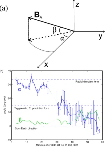
Fig. 4.The orientation of the ambient magnetic field at the Cluster
site. (a)Definition of the anglesαandβ. The axes represent the
GSM coordinate system. (b)The orientation of the ambient
mag-netic field as a function of time, obtained from minimum/maximum variance analysis. The lines are the averages of the results from the four spacecraft and the error bars show their standard
devia-tion. Those data points where the standard deviation exceeds 20◦
are omitted.
This suggests that there was an intensification of reconnec-tion about 12 min after its first onset.
2.2 Ambient field direction
Figure 3 shows a very clear anticorrelation betweenBx and By until about 03:25. Similarly the x and y components of proton velocity exhibit a clear anticorrelation during the out-flows. After the event the correlation is not so clear.
Figure 4 examines more closely how the orientation of the ambient magnetic field changes. The two anglesαandβthat describe the orientation are illustrated in the upper panel: β is the angle between the ambient field and thexyplane, and αis the angle between the x-axis and the projection of am-bient field in thexyplane. In the lower panel the angles are calculated as a function of time using maximum/minimum
variance analysis (MVA). For each data point, a five minutes long data interval was used to calculate the MVA eigenvec-tors. The angles were calculated from the eigenvector having the smallest angle with the x-axis; in most cases this was the maximum variance eigenvector. The result is consistent with the average direction of the field itself during intervals when Cluster stays away from the central current sheet. However, long enough such intervals only occur before the start of re-connection and therefore MVA is needed to follow the time evolution of the ambient field direction.
The curves in Fig. 4b show the average of the results from the four spacecraft, and the error bars in theαcurve repre-sent their standard deviation. The bars are omitted from the β curve for clarity, but they would be similar in magnitude as those forα. The deviations reflect short-timescale vari-ations in the magnetic field direction near the current sheet centre, due to tilted orientations of the current sheet during oscillations. However, the purpose of Fig. 4b is not to bring out all these variations but rather to assess the slow change in the background field on as global a scale as possible. Five minutes long data intervals were used in order to average out the effects of individual flappings.
Until 03:24 the four spacecraft give well consistent re-sults: The α angle is rather large, about 30 degrees, and stays roughly constant with some minor variations.βis very small, which means that the ambient field is quite accurately in thexy plane. Between 03:24–03:29 the results from the four spacecraft are wildly varying and inconsistent with each other. This is because Cluster stayed in the central current sheet and did not see the ambient lobe field. After 03:29 the analysis produces again meaningful results, but the differ-ences between the different spacecraft are now considerably larger reflecting the sub-Cluster-scale variations in the mag-netic field. Despite the resulting inaccuracy one can see that αis now smaller and still decreases during the event.
One more caveat must be mentioned regarding the inter-pretation of αbetween 03:31–03:36. During this time the Hall fields may affect the analysis: earthward of the x-line they tend to makeαsmaller, and they persisted in that sense for most of the period. However, overall one can conclude that before the onset of reconnection the ambient magnetic field was oriented approximately radially, but became almost aligned with the x-axis during the event.
they are causally connected. This question will be discussed further in Sect. 5.1.
2.3 Choosing the natural coordinate system
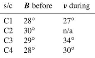
The preceding analysis indicates that the GSM coordinate system is not very good for studying the event: a more natu-ral coordinate systemx′y′z′would be one in which the out-flows and ambient lobe fields are aligned with thex′ axis. As the ambient magnetic field direction changes during the event, the choice is ambiguous. To get another hint, we ex-amine the proton bulk velocity. We find the smallest coor-dinate rotation angleαthat removes thevx-vycorrelation in the time period 03:25–03:43, which is the shortest time in-terval including both the observed outflows. The results are given in the right column of Table 1. The result stays the same even if the period 03:31–03:35, when the velocity mo-ments are not relevant, is removed from the data. The table also gives angles of no correlation based on magnetic fields measurements. These have been calculated using the pre-reconnection interval 03:00–03:25.
It is interesting that although the orientation of the ambi-ent lobe fields changes considerably during the reconnection event, the direction of both outflows is quite accurately that of the original ambient fields. This suggests that the local reconnection geometry may stay in the original orientation while global field orientation is already changing towards the x-direction. We thus choose to align our basic coordinate system with the pre-reconnection ambient field, and rotate the GSM system 29 degrees clockwise around the z-axis to accomplish that. Because the ambient field is very close to thexyplane, we leave thez′axis to be the same as the z-axis.
3 X-line
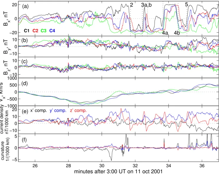
Figure 5 gives an expanded view of the early and middle phases of the reconnection event. The bottom panel shows the components of the magnetic curvature vector. Its x-component is negative, that is, the curvature is tailward un-til about 03:31:20, when strong earthward curvature is sud-denly observed. After this initial spike the calculated curva-ture stays around zero for several minutes; this is because the entire Cluster constellation stays mostly on one or the other side of the current sheet centre, as evidenced by theBx com-ponents in panel (a). Each time when Cluster crosses the cur-rent sheet a “spike” of earthward curvature is observed. Our interpretation is that these spikes reflect a constant earthward curvature at the centre of the thin current sheet. Qualitatively the curvature data indicate that an x-line passed Cluster at 03:31:20.
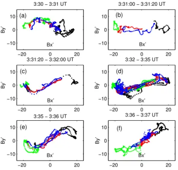
Corroborative evidence is provided by the Hall fields. Fig-ure 6 illustrates the point by comparing statisticallyBy′ ver-susBx′. Until 03:30 UT no Hall signature is visible. Between 03:30 and 03:31 the data show a clear quadrupolar variation
Table 1.The angle of coordinate rotation in thexyGSMplane that
removes the correlation betweenBx′ andBy′ before the event,
in-terval 03:00–03:25 UT, or betweenvx′ and vy′ during the event,
interval 03:25–03:43 UT.
s/c Bbefore vduring
C1 28◦ 27◦
C2 30◦ n/a
C3 29◦ 34◦
C4 28◦ 30◦
inBy′ (panel a). The sense of the variation is such that near the current sheet centreBy′andBx′anticorrelate, which cor-responds to the tailward side of x-line of the Hall structure. Then at 03:31:00 the Hall signature disappears for about 20 s (panel b). At 03:31:20 a clear Hall signature appears again (panel c), but its sense has been reversed and corresponds now to the earthward side of reconnection line.
During the next three minutes (panel d in Fig. 6) the statis-tical picture is somewhat cluttered because the current sheet undergoes flapping motions with strongly tilted orientations. It will be shown in the next subsection that the Hall structure is tilted with the current sheet during many of the crossings. At those instants the Hall signature is found mainly inBz′, and is thus not revealed by Fig. 6. Also, some of the correla-tion visible in panel (d) may be due to the orientacorrela-tion change of the lobe fields as discussed in the previous section. How-ever, to the extent that any Hall signature is observable, it retains its earthward of x-line -sense during this period.
At 03:35–03:36 a clear and strong quadrupolar Hall sig-nature is again observed (Fig. 6e). This coincides with the first rapid earthward acceleration of protons (Fig. 5d). Af-ter 03:36 a strong correlation betweenBx′ andBy′ remains and persists also after the time interval shown, but it is due to the ambient field orientation change discussed in Sect. 2.2. We thus interpret the interval 03:30–03:36 as the time that Cluster spent in the diffusion region, because during this in-terval it was between the outflow jets and recorded Hall sig-natures. Only one x-line passing was observed at about 3:31, but the possibility of multiple x-lines cannot be completely ruled out.
4 Current sheet crossings
4.1 Before, during and after reconnection
−20 0 20
B
x, nT
−10 0 10
B
y, nT
−10 0 10
B
z, nT
−1000 −500 0 500 1000
v
x, km/s
−10 0 10 20
current density nT/1000 km
26 28 30 32 34 36
−5 0 5
curvature 1/(1000 km)
minutes after 3:00 UT on 11 oct 2001
2 3a,b
4a 4b
5
(
a
)
(
b
)
(
c
)
(
d
)
(
e
)
(
f
)
C1 C2 C3 C4
x’ comp. y’ comp. z’ comp.
Fig. 5.Observed and calculated quantities during the event, given in thex′y′z′coordinate system defined in Sect. 2.4.(a–c)Magnetic field
components. Data from Cluster 1 in black, C2 in red, C3 in green and C4 in blue. (d)x component of proton flow velocity, colours as in
(a–c). Proton data from C2 is missing because its CIS instrument group is broken.(e)Current density and(f)curvature vector at the Cluster
barycentre.x′component in black,y′in blue andz′in red.
On three occasions an oscillation passes all the four Clus-ter spacecraft so that the orientation and normal velocity of the moving current sheet can be determined by multi-point timing analysis. The crossing pairs are marked in Fig. 3, pair 4 also in Fig. 5. Table 2 shows the timing results. The validity of the current sheet normal directions was checked by MVA and by comparing them to the current density vec-tors given by the curlometer method (Dunlop et al., 2002).
The normal velocities are remarkably similar within each pair of crossings. Around 03:09 when the current sheet is in a relatively quiet state, it passes Cluster first upward and later downward with a velocity of about 60 km/s. The next double crossing (number 4) occurs during reconnection, in the thin current sheet of the diffusion region, and has speeds
−20 0 20 −10
0 10
Bx’
By’
3:30 − 3:31 UT
−20 0 20
−10 0 10
Bx’
By’
3:31:00 − 3:31:20 UT
−20 0 20
−10 0 10
Bx’
By’
3:31:20 − 3:32:00 UT
−20 0 20
−10 0 10
Bx’
By’
3:32 − 3:35 UT
−20 0 20
−10 0 10
Bx’
By’
3:35 − 3:36 UT
−20 0 20
−10 0 10
Bx’
By’
3:36 − 3:37 UT
(a) (b)
(c) (d)
(e) (f)
Fig. 6. By′ versusBx′ in six consecutive time intervals during the
reconnection event, illustrating the Hall effect. The colours refer to different spacecraft: data from Cluster 1 is in black, C2 in red, C3 in green and C4 in blue.
Table 2. The normal vector and the normal velocity of the cur-rent sheet in three pairs of crossings, marked in Fig. 3. The
nor-mal vector components are given in GSM ([x, y, z]) and rotated
([x′, y′, z′]) coordinates. The results have been obtained by timing
analysis.
[nx, ny, nz] [nx′, ny′, nz′] vn(km/s)
1a [.22,−.02, .97] [.20,−.09, .97] 56
1b [.09, .86,−.50] [−.33, .80,−.50] 60
4a [.32, .94, .10] [−.18, .98, .10] 177
4b [.49, .67, .56] [.10, .82, .56] 157
6a [.05, .32, .95] [−.11, .30, .95] 118
6b [−.24, .97, .01] [−.68, .73, .01] 117
these oscillations about 10 s after the other three spacecraft, and as Cluster 2 is located about 1000 km duskward of the other satellites (Fig. 1b), this indicates that the oscillations are travelling duskward with an order-of-magnitude velocity of 100 km/s. Together with the observed period this leads to the order-of-magnitude estimate of 1RE for the wavelength of the oscillations.
4.2 Bz′variations from tilted Hall fields
They′andz′components of the magnetic field show rather strong small-scale fluctuations during the entire event. Many
15 20 25 30 35 40 45 50 55 60
−20 −10 0 10 20
Bx’ = Bl
Crossing 4b, time−shifted
−10 0 10
By’
Base coordinates
15 20 25 30 35 40 45 50 55 60
−10 0 10
Bz’
−10 0 10
Bm
Coordinates adapted to the crossing
15 20 25 30 35 40 45 50 55 60
−10 0 10
Bn
seconds after 3.34 UT on 11 October 2001
Fig. 7.The magnetic field components measured by Cluster during the crossing 4b in Fig. 5. The data have been time-shifted so that the
Bx′=Blsign changes coincide; the time axis gives real time for C1.
In the two lowermost panels the coordinates have been rotated to
show the Hall effect inBm. Colouring of the lines as in Figs. 5a–c
and 6.
of the strongest fluctuations in Bz′ coincide with Bx′ sign changes and consist of a negative peak followed immediately by a positive one. Figure 7 examines in detail one such cross-ing, 4b in Table 2 and Fig. 5. The data from Cluster 2, 3 and 4 are time-shifted so that theBx′sign changes coincide.
The first three panels show the magnetic field components during the crossing in the coordinates x′y′z′, same as in Fig. 5. Bipolar variation is seen in bothBy′ andBz′. Then another rotation of 43◦, in a left-handed sense around the
Table 3. The unit base vectors of the two specialised coordinate
systemsx′y′z′andlmn, given in GSM coordinates.
xGSM yGSM zGSM
ˆ
x′ 0.875 –0.485 0
ˆ
y′ 0.485 0.875 0
ˆ
z′ 0 0 1
ˆ
l 0.875 –0.485 0
ˆ
m 0.355 0.640 –0.682
ˆ
n 0.331 0.596 0.731
In the new coordinate system there is almost no variation inBn until 03:34:35, which confirms that the chosen coor-dinate system is well fitted to the crossing. The Hall signa-ture was recognizable already inBy′, but inBmit is stronger and clearer. Note especially the data of Cluster 3 (green) after crossing the current sheet centre: |Bm| increases di-rectly proportionally to|Bl|untilBl reaches about−10 nT. When Cluster 3 travels farther into the southern lobe,|Bm| decreases and vanishes whenBlreaches about−20 nT. The other three satellites stay closer to the current sheet centre, and consequently their measured Bm values stay negative considerably longer after the crossing.
We searched for Hall effects also from all the other cross-ings 2–5 marked in Fig. 5. We used both correlation-minimizing rotations around thex′axis only and MVA coor-dinates. Clear Hall effects were found from all the crossings except 3a and 3b, in which the Hall fields were only barely recognizable. The double crossing 3 was more difficult to treat than the others, because three of the spacecraft crossed the current sheet only half-way and the return to the southern side was immediate (Cluster 3 did not cross at all).
In a majority of the crossings the coordinate transforma-tion that brought out the Hall fields in the second (m) com-ponent ofBalso made variation in the third (n) component ofB relatively small. This was the case in crossings 2, 3a, 4b and 5. In 3b and 4a there remain variations inBnthat are about as large as the Hall effect inBm. We thus conclude the following: during the reconnection event under examina-tion Cluster stays several minutes in the diffusion region and sees there strong wave-like oscillations of the current sheet, which propagate duskward. Hall fields can be recognized in connection with the crossings, and they are in an orienta-tion tilted along the current sheet. This explains most of the largest fluctuations inBz′, but in addition to flapping and Hall fields there is considerable irregular small-scale variation in the magnetic field.
Fig. 8.A schematic illustration of how the orientation of the mag-netic field in the tail may have changed due to the reconnection event. An x-line and outflows are also drawn. The figure shows a
view looking down on thexyplane.
5 Discussion and conclusions
5.1 A global configuration change in the tail due to recon-nection?
deflection thus signifies a large scale configuration change in the tail. At the time there were no other satellites that could provide magnetometer data from the magnetotail, so we do not know whether this configuration change was truly global and affected also the post-midnight part of the tail. Figure 8 that illustrates the configuration change has been drawn as-suming symmetry in the y-direction.
Solar wind data from the ACE and WIND satellites show that this change was not caused directly by the solar wind; in particular, the IMF y-component stays almost constant at +4...+5 nT during the entire event. The solar wind veloc-ity and the dynamic pressure also show only slight variations (see Fig. 2). IMF z-component changed from positive to neg-ative around 03:20 UT, but the change was gradual and too slow to be considered as the direct cause of the observed fast orientation change. The change was therefore most proba-bly associated with the reconnection that started at the same time.
Simultaneous ground signatures were also observed by three Canadian magnetometer stations. A southward deflec-tion of about 150 nT was recorded at Gillam and Poste de la Baleine at 03:27 UT – at the same time when Goes-8 ob-served the deflection inBy – and a couple of minutes later also at Fort Churchill (Fig. 2e). The magnetic signature was a clear indication of a westward electrojet. Gillam and Poste de la Baleine have the same magnetic latitude but are sep-arated by 25◦ in longitude, Gillam being the more western station, while Fort Churchill is 2.3◦to the north from Gillam. The disturbance was thus propagating northward but did not advance to the stations north of Fort Churchill. Nor was it observed on more eastern or western stations. According to the Tsyganenko 96 model Fort Churchill was near to the magnetic footpoint of Cluster and Poste de la Baleine near to that of Goes-8. The question is thus left open, whether this phenomenon was tail-wide or limited to the sector in which Cluster and Goes-8 were.
The Tsyganenko 2001 model predicts that the angle be-tween the magnetic field and x-axis at the Goes-8 location should be 22◦. This is consistent with the measured angle before the deflection at 03:27. At the Cluster location T01 predicts an ambient field angle of about 15◦, which is con-sistent with the MVA result at 03:30, immediately after the initial deflection but before the subsequent gradual change. Thus, before the onset of reconnection the tail widens at the Cluster site more than the model predicts, but during the re-connection event the field both at the Cluster and Goes-8 sites becomes more aligned with the x-axis than in the model.
What may have caused this tail configuration change? It was not compression by solar wind or penetration of IMF y-component. Dipolarization also occurs at Goes-8, but only about 12 min later, so this was something different. The onset of reconnection (timed from the start of the tailward flow at Cluster), the configuration change at Cluster and at Goes-8, and the commencement of a westward electrojet in the
ionosphere were all practically simultaneous: time-ordering cannot be established from the observations.
We hypothesize that a large-scale instability involving field-aligned currents coupling to the ionosphere is respon-sible for the onset of reconnection and the simultaneous con-figuration change. Either release of stress associated with the current disruption or the tailward motion of the x-line then led to the field rotation from radial to one aligned with the Sun–Earth line. Reconnection also caused flux to pile up in the earthward side causing the field dipolarization.
5.2 X-line at the edge of the diffusion region
In Sect. 3 we showed that Cluster was in the diffusion re-gion between the outflow jets during 03:30–03:36 and that an x-line passed Cluster at about 03:31, that is, much sooner than halfway in the diffusion region. There are at least four possible reasons to this:
1. The x-line was near the edge of the diffusion region. In that case the x-line ”leads” the tailward motion of the reconnection and ”drags” the diffusion region behind. Protons become demagnetized for a relatively long time in those regions through which the x-line has passed. 2. The diffusion region is symmetric but spreads out as the
reconnection site grows older. Cluster recorded the tail-ward half of the diffusion region soon after the onset of reconnection, but when it was in the earthward half the diffusion region grew so much wider that it took much longer before its earthward edge reached Cluster. 3. The reconnection region moves tailward at a changing
speed or stepwise. In this event, it moved first quickly but then just happened to stop for a few minutes when the x-line had passed Cluster. The reconnection region may have stopped another time at 03:36–03:39, which would explain the apparent two steps in the earthward acceleration (see Fig. 3).
4. The diffusion region had multiple x-lines, but only the most tailward one happened to be clearly observable in the magnetometer recordings. The other x-line(s) may have passed when Cluster was away from the current sheet centre.
Decisive discrimination between these hypotheses would re-quire observing the reconnection site at two or more different xvalues on its way tailward.
5.3 Hall fields conform to current sheet kinks
B
LobeB
Hally
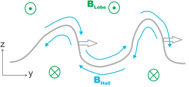
z
Fig. 9.A schematic illustration of duskward-propagating kinks in the current sheet. The ambient magnetic field direction is shown in green, while the Hall fields are in blue. The Hall fields stay adjacent to the current sheet and conform to its kinks.
when the current sheet turns from quiet to disturbed state: before reconnection onset the current sheet passes Cluster at a speed of about 60 km/s, during reconnection at 170 km/s and after reconnection at 120 km/s. The current sheet normal has a largey′component during most of these crossings, in-dicating that the current sheet is strongly tilted away from the xyplane.
There are many quite large-amplitude fluctuations inBz′ during this reconnection event, especially within the diffu-sion region (Fig. 5). That kind of fluctuations are often in-terpreted as signatures of plasmoids or flux ropes, or said to signify filamentation of the cross-tail current associated with current disruption model (see, e.g., Lui et al., 2005). How-ever, it was shown in Sect. 4.2 that in this event most of the largest fluctuations are caused by Hall fields. They appear as variations inBz′, instead of only inBy′, because in many crossings the current sheet is in a strongly tilted orientation. This also indicates that examination ofByis not always suffi-cient to establish the presence or absence of Hall fields. Fig-ure 9 illustrates how the quadrupolar Hall structFig-ure conforms to the waves propagating in the current sheet.
Acknowledgements. We thank H. Singer at NOAA SEC for the
GOES-8 magnetometer key parameter data, N. Ness at Bartol Re-search Institute for ACE magnetometer data, and D. J. McComas at Southwest Research Institute for ACE SWEPAM data. These satel-lite data were obtained through the CDAWeb. We also acknowledge D. Belian (PI) and G. D. Reeves for providing the LANL SOPA energetic electron data, Canadian Space Agency for the GILL and FCHU magnetometer data and Geological Survey of Canada for the PBQ magnetometer data.
T. V. Laitinen thanks N. Partamies for help with the ground mag-netometer data, T. I. Pulkkinen for reading and commenting the manuscript, N. Ganushkina for help with the Tsyganenko models, and K. Kauristie, M. Palmroth and H. Koskinen for inspiring
dis-cussions in Finnish. The work of T. V. Laitinen was supported by the Magnus Ehrnrooth foundation and his visit to the IWF by the Vilho, Yrjö and Kalle Väisälä foundation.
Topical Editor I. A. Daglis thanks L. Zelenyi and A. Vaivads for their help in evaluating this paper.
References
Asano, Y., Mukai, T., Hoshino, M., Saito, Y., Hayakawa, H., and Nagai, T.: Evolution of the thin current sheet in a sub-storm observed by Geotail, J. Geophys. Res., 108(A5), 1189, doi:10.1029/2002JA009785, 2003.
Baker, D. N., Pulkkinen, T. I., Angelopoulos, V., Baumjohann, W., and McPherron, R. L.: The neutral line model of substorms: Past results and present view, J. Geophys. Res., 101, 12 975–13 010, 1996.
Balogh, A., Carr, C. M., Acuña, M. H., et al.: The Cluster Magnetic Field Investigation: overview of in-flight performance and initial results, Ann. Geophys., 19, 1207–1217, 2001,
http://www.ann-geophys.net/19/1207/2001/.
Baumjohann, W., Paschmann, G., and Luhr, H.: Characteristics of high-speed ion flows in the plasma sheet, J. Geophys. Res., 95, 3801–3809, 1990.
Belehaki, A., McEntire, R. W., Kokubun, S., and Yamamoto, T.: Magnetotail response during a strong substorm as observed by GEOTAIL in the distant tail, Ann. Geophys. 16, 528–541, 1998. Deng, X. H., Matsumoto, H., Kojima, H., Mukai, T., Anderson, R. R., Baumjohann, W., and Nakamura, R.: Geotail encounter with reconnection diffusion region in the Earth’s magnetotail: Evi-dence of multiple X lines collisionless reconnection?, J. Geo-phys. Res., 109, A05206, doi:10.1029/2003JA010031, 2004. Dunlop, M. W., Balogh, A., Glassmeier, K.-H., and Robert,
Eastwood, J. P., Sibeck, D. G., Slavin, J. A., Goldstein, M. L., Lavraud, B., Sitnov, M., Imber, S., Balogh, A., Lucek, E. A., and Dandouras, I.: Observations of multiple X-line structure in the Earth’s magnetotail current sheet: A Cluster case study, Geo-phys. Res. Lett. 32, L11105, doi:10.1029/2005GL022509, 2005. Hones Jr., E. W., Birn, J., Baker, D. N., Bame, S. J., Feldman, W. C., McComas, D. J., Zwickl, R. D., Slavin, J. A., Smith, E. J., and Tsurutani, B. T.: Detailed examination of a plasmoid in the distant magnetotail with ISEE 3, Geophys. Res. Lett. 11, 1046– 1049, 1984.
Hoshino, M., Nishida, A., Mukai, T., Saito, Y., Yamamoto, T., and Kokubun, S.: Structure of plasma sheet in magnetotail: Double-peaked electric current sheet, J. Geophys. Res., 101, 24 775– 24 786, 1996.
Laitinen, T. V., Pulkkinen, T.I., Palmroth, M., Janhunen, P., and Koskinen, H. E. J.: The magnetotail reconnection region in a global MHD simulation, Ann. Geophys., 23, 3753–3764, 2005, http://www.ann-geophys.net/23/3753/2005/.
Lui, A. T. Y, Meng, C.-I., and Akasofu, S.-I.: Wavy nature of the magnetotail neutral sheet, Geophys. Res. Lett., 5, 279–282, 1978.
Lui, A. T. Y., Jacquey, C., Lakhina, G. S., Lundin, R., Nagai, T., Phan, T.-D., Pu, Z. Y., Roth, M., Song, Y., Treumann, R. A., Yamauchi, M., and Zelenyi, L. M.: Critical issues on magnetic reconnection in space plasmas, Space Sci. Rev., 116, 477–521, doi:10.1007/s11214-005-1987-6, 2005.
Nagai, T.: Location of magnetic reconnection in the magnetotail, Space Sci. Rev., 122, 39–54, doi:10.1007/s11214-006-6216-4, 2006.
Pulkkinen, T. I., Palmroth, M., Tanskanen, E. I., Janhunen, P., Kosk-inen, H. E. J., and LaitKosk-inen, T. V.: New interpretation of magne-tospheric energy circulation, Geophys. Res. Lett., 33, L07101, doi:10.1029/2005GL025457, 2006.
Rème, H., Aoustin, C., Bosqued, J. M., et al.: First multispacecraft ion measurements in and near the Earth’s magnetosphere with the identical Cluster ion spectrometry (CIS) experiment, Ann. Geophys., 19, 1303–1354, 2001,
http://www.ann-geophys.net/19/1303/2001/.
Runov, A., Sergeev, V.A., Nakamura, R., Baumjohann, W., Zhang, T.L., Asano, Y., Volwerk, M., Vörös, Z., Balogh, A., and Rème, H.: Reconstruction of the magnetotail current sheet structure us-ing multi-point Cluster measurements, Planet. Space Sci., 53, 237–243, 2005.
Sergeev, V. A., Semenov, V. S., and Sidneva, M. V.: Impulsive re-connection in the magnetotail during substorm expansion, Planet Space Sci. 35, 1199–1212, 1987.
Sergeev, V., Runov, A., Baumjohann, W., Nakamura, R., Zhang, T. L., Volwerk, M., Balogh, A., Rème, H., Sauvaud, J. A., André, M., and Klecker, B.: Current sheet flapping motion and struc-ture observed by Cluster, Geophys. Res. Lett. 30, 1327–1330, doi:10.1029/2002GL016500, 2003.
Sergeev, V., Runov, A., Baumjohann, W., Nakamura, R., Zhang, T. L., Balogh, A., Louarnd, P., Sauvaud, J.-A., and Rème, H.: Ori-entation and propagation of current sheet oscillations, Geophys. Res. Lett. 31, L05807, doi:10.1029/2003GL019346, 2004. Shay, M. A., Drake, J. F., Swisdak, M., Dorland, W., and Rogers,
B. N.: Inherently three dimensional magnetic reconnection: A mechanism for bursty bulk flows?, Geophys. Res. Lett., 30(6), 1345, doi:10.1029/2002GL016267, 2003.
Sonnerup, B. U. Ö.: Magnetic reconnection, in Solar System Plasma Physics, vol. 3, edited by: Lanzerotti, L. J., Kennel, C. F., and Parker, E. N., pp. 45–108, North-Holland, New York, 1979. Thompson, S. M., Kivelson, M. G., El-Alaoui, M., Balogh, A.,