in Complex Scenes
Gonzalo H. Otazu1,2*, Christian Leibold1,2
1Division of Neurobiology, Department Biology II, Ludwig-Maximilians-Universita¨t, Munich, Germany,2Bernstein Center for Computational Neuroscience, Munich, Germany
Abstract
The identification of the sound sources present in the environment is essential for the survival of many animals. However, these sounds are not presented in isolation, as natural scenes consist of a superposition of sounds originating from multiple sources. The identification of a source under these circumstances is a complex computational problem that is readily solved by most animals. We present a model of the thalamocortical circuit that performs level-invariant recognition of auditory objects in complex auditory scenes. The circuit identifies the objects present from a large dictionary of possible elements and operates reliably for real sound signals with multiple concurrently active sources. The key model assumption is that the activities of some cortical neurons encode the difference between the observed signal and an internal estimate. Reanalysis of awake auditory cortex recordings revealed neurons with patterns of activity corresponding to such an error signal.
Citation:Otazu GH, Leibold C (2011) A Corticothalamic Circuit Model for Sound Identification in Complex Scenes. PLoS ONE 6(9): e24270. doi:10.1371/ journal.pone.0024270
Editor:Olaf Sporns, Indiana University, United States of America
ReceivedMarch 29, 2011;AcceptedAugust 7, 2011;PublishedSeptember 13, 2011
Copyright:ß2011 Otazu, Leibold. This is an open-access article distributed under the terms of the Creative Commons Attribution License, which permits unrestricted use, distribution, and reproduction in any medium, provided the original author and source are credited.
Funding:This work was supported by the Bundesministerium fu¨r Bildung und Forschung (BMBF) under grant number 01GQ0440 (Bernstein Center for Computational Neuroscience, Munich). The funders had no role in study design, data collection and analysis, decision to publish, or preparation of the manuscript.
Competing Interests:The authors have declared that no competing interests exist. * E-mail: [email protected]
Introduction
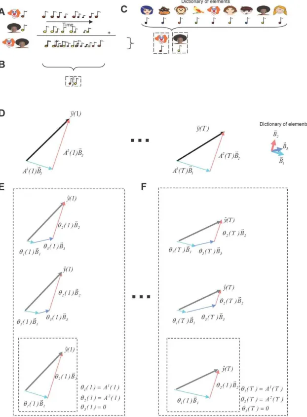
Auditory scenes are generally composed of sounds produced by multiple sources. The observed complex auditory signal is a superposition of these sources, making the identification of the individual sound elements a non-trivial problem (Fig. 1A). While humans generally perform better than machines do in recognizing auditory objects in complex scenes, it is not yet known how our nervous system performs this task in real time.
In one family of computer algorithms, the blind source separation algorithms (Fig. 1B), source elements are identified using only the information extracted from the observed signal. These approaches make no parametric assumptions about the superimposed signals in the auditory scene. Without such prior information, the amount of data necessary to identify the sources present in a scene is large, making them not compatible with the real time requirement for biological systems.
An alternative family of computer algorithms assumes that the elements that are present in a scene belong to a large, but finite, dictionary of known sounds (Fig. 1C) [1,2,3,4,5,6]. By making this assumption, the number of observations required to identify a source is substantially reduced, making them more suitable for biological systems. These algorithms assume that the observed auditory scene originated by a time-varying linear combination of just a few elements that belonged to the dictionary (Fig. 1D). Then, the dictionary elements are selected such that an appropriate linear combination would reconstruct the observed signal with the highest fidelity. As the elements present in an auditory scene have to be part of the dictionary, these algorithms require a very large number of dictionary elements. However, if the dictionary is large enough, there are
multiple combinations of elements that would reconstruct the observed signal with the same high fidelity (Fig. 1E–F). To enforce uniqueness of the solution, those algorithms require additional minimization of a secondary cost function. Since a typical auditory scene is composed of only few elements, this secondary objective is taken as the number of active dictionary elements. Due to this additional cost function the number of identified dictionary elements is small, and therefore these algorithms provide possible models for sparse codes in sensory brain regions [7].
A particular auditory scene activates only a few from the large number of neurons available in the auditory cortex [8,9,10,11,12], which matches the behavior of sparse coding algorithms. However, we do not know which of these algorithms the auditory system really implements, and what are the mechanisms the brain uses to select the dictionary elements that are present in a scene.
Figure 1. Identification of sources present in complex auditory scenes using large dictionaries.(A) Auditory scenes are composed of sounds generated by different sources. (B) Blind source separation methods estimate the sources present in a scene based only on the observed scene. (C) Other algorithms assume that the sources present in a scene are part of a very large dictionary of possible sources (represented by the collection of pictures and the associated sounds). (D) These algorithms also assume that the sources present are combined linearly, (vectors~BBkmultiplied by the time varying amplitudeAk(t)), to generate the time varying scene (time-varying vector~yy(t)). (E) Algorithms as inDcreate an estimate of the observed signal by combining elements of the dictionary, each one weighted by an time varying estimated parameterhk(t). For large dictionaries, there are multiple estimated parameters that create an estimate of the observation that matches equally well to the observed signal (represented by the different combinations of vectors inside the large square that generate the same well-matched estimate^yy(t)). A single solution is chosen by minimizing the number of active dictionary elements (vector combination inside the smaller square). (F) At each time step, a new set of parametershk(t)is estimated that reflect the contribution of the identified dictionary element to the current auditory sceneAk(t). The other estimated parametersh
Results
CPA works on superimposed sound sources
CPA uses similar assumptions as previous source identification algorithms (Fig. 1D), mainly that the stimulus originated from linear combination of the sources [1,2,3,4,5,6]. For illustrative purposes, we will assume an auditory scene where each sound source k has a characteristic frequency spectrum ~BBk, which is
stationary over time [13]. For non-stationary spectra the feature vectors ~BBk may also be generalized to the spectrotemporal
domain, or even to include higher order cues of complex signals like speech. The shape of the spectrum originating from each source is assumed to be stationary, but the amplitude Ak(t)
fluctuates in time (Text S1: Definition of auditory scene), that is at any instantt, the superposition of several of these sources creates the observed signal~yy(t).
~yy(t)~A1(t)B1~B zA2(t)~BB2zA3(t)~BB3z:::zAn(t)~BBn ð1Þ
We assume that each source generates its sounds independently of other sources. Therefore, the amplitude modulationsAk(t)of
the different objects are uncorrelated. We assume that the system has previously learned a large dictionary of n possible sound elements~BBi(n..f, wherefis the number of features of the signal ~yy(t), in this case,fwill be the number of frequency bands of the spectrum) that includes the sources~BBk that generated the signal ~yy(t). CPA receives as inputTsamples of the observed signal~yy(t)
and, based on temporal fluctuations of the contributing dictionary elements [14], outputs a unique set of parameters hi, i = 1..n
(Fig.2). The parametershiestimated by CPA will take the value of
one, if the corresponding dictionary element is part of the auditory scene, or zero, if it is not.
CPA finds a unique set of presence parameters by minimizing estimation error
Similar to previous algorithms [1,2,3,4,5,6], CPA creates an estimate^yy(t)about the current auditory scene and determines the parametershiby finding the set of parameters that minimize the
square error between the estimate ^yy(t) and the observed signal ~yy(t). Previous algorithms’ estimates^yy(t)had the same structure as the model of the auditory scene, mainly (cf.equation 1)
^ y
y(t)~h1(t)~BB1zh2(t)~BB2z:::hn(t)~BBn ð2Þ
There are two main differences of CPA with such previous algorithms. The first one is the way the estimate^yy(t)is generated. The CPA estimate is
^ y
y(t)~h1(~yy(t):~BB1)~BB1zh2(~yy(t):~BB2)~BB2z:::hn(~yy(t):~BBn)~BBn ð3Þ
Each dictionary element is additionally weighted with its similarity ~yy(t):~BBi; forming the time-varying projection of the
vector~yy(t)onto the vector~BBi(Fig. 2AandText S2: Corrected projections algorithm). The second difference is in the way that multiple observations are processed. In the standard algorithms, the estimated parameters hi(t) are generated at the
sampling rate of the input. In contrast, CPA estimates a single set of parameters hi for all T observed samples (Fig. 2B). CPA
estimated parameters do not indicate the instantaneous contri-bution of a dictionary element, but its presence or absence in an
auditory scene (Fig. 2C). Therefore, we called the CPA parametershipresence parameters.
The inclusion of the similarities~yy(t):~BBiin the estimate^yy(t)is the
key element that causes this minimization to yield a unique set of presence parameters hi, without requiring any additional
con-straints (Text S2: Corrected projections algorithm). This uniqueness property of CPA contrasts to other algorithms that require additional constraints to find unique solutions [1,2,3,4,5,6].
CPA presence parameters are binary variables that indicate the presence of known sound sources in a scene
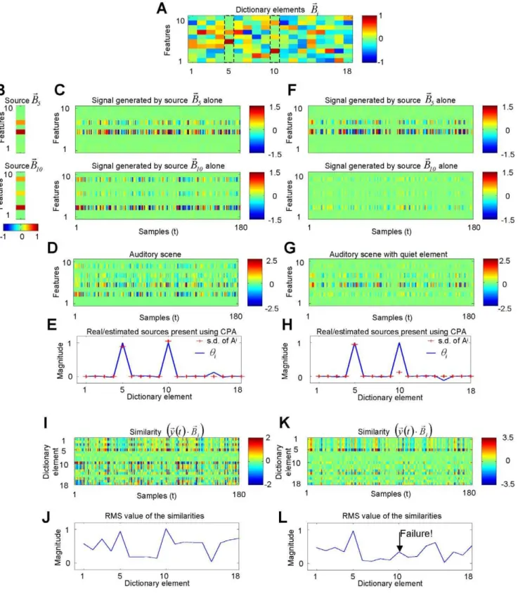
If signals that match the sources in the scene are part of the dictionary (Fig. 3A), and if the sources present~BBkare orthogonal,
minimizing the average error will identify sources present in a scene by finding the correct set of the presence parameters hi
(Fig. 3B–E). A correct identification consists of hk= 1for each
one of the few sources participating in the scene andhi= 0for the
large number of dictionary elements that are not part of the scene (Text S3: Proof that CPA detects the elements present in a mixture). This typical binary behavior of the presence parametershi makes apparent that CPA works as a recognition
algorithm, meaning it finds specific dictionary elements represent-ing identified sources. Although the orthogonality requirement seems restrictive, it applies only to the dictionary elements~BBkthat
are present in a particular scene and not to the whole dictionary, which would have limited the number of dictionary elements to the number of features of the dictionary elements. Moreover, CPA is robust to small deviations from orthogonality in the present sources ~BBk, which is the case for most pairs of vectors if the
number of featuresfof the input signal is large enough, potentially allowing the use of very large dictionaries (seeText S4: Effects of auditory scene complexity and dictionary size on CPA performanceand Fig. S1 for a case in which there is more overlap). If the sources in a scene can be represented by orthogonal elements, a common approach is to estimate them using Principal Component Analysis (PCA). However, PCA might require larger amounts of input data than CPA because PCA does not incorporate prior information from a dictionary (Fig. S2).
The presence parameters of CPA indicate the presence or absence of learned sound objects that are already part of the dictionary. An element that has not been encountered before will not be recognized, as there won’t be a single presence parameter with a value of 1 indicating its participation in the scene. Instead, it will appear as small values over multiple presence parameters (Fig. S3).
CPA estimated parameters are invariant to sound intensity
CPA still identifies the elements present (Fig. 3F–H), even if the contribution of one of the sources is quieter than the other sources. The presence parameters hi hence indicate the presence or
absence of a source~BBi, independent of the magnitudeAi(t)of the
source’s contribution to the auditory scene, for all observed T
samples. This is different from previous algorithms [1,2,3,4,6], which would have yielded a time-varying parameters hi(t) that
indicates the instantaneous contribution of the corresponding dictionary element ~BBi to the auditory scene at that moment in
time.
CPA solves problems that cannot be solved by template matching
of the scene is a superposition of multiple objects. A standard method for pattern recognition, template matching, identifies the sources present in a scene by calculating how similar the instantaneous spectrum~yy(t) is to each of the n possible sound sources and identifying the sources present as the most similar ones. When the contributions of the present sources to the signal ~yy(t)are equally large, we can recognize that the elements~BBiwith
the largest similarity~yy(t):~BBiare the elements that participated in
the mixture (Fig. 3I–J). However, the similarities give a more ambiguous picture of the elements present than the presence parameters of CPA (compareFig. 3EwithFig. 3J). In the case where one of the elements is quieter than the other (Fig. 3F–H), the similarities fail to identify the more quiet source (Fig. 3K–L), as the observed scene is more similar to other dictionary elements that were not present than to the more quiet element that participated in the scene.
Iterative implementation of CPA is computationally efficient
The original formulation of CPA is not a realistic model for the brain’s sensory system because it requires storing all the T
observations of an auditory scene. The original CPA also cannot handle dictionaries with large number n of elements because it requires the inversion of a square matrix ofndimensions, which is numerically ill- conditioned for large n (Text S2: Corrected
projections algorithm). However, the fact that in CPA the minimization of the difference between the observed signal~yy(t)
and the estimate of that signal^yy(t)yields a single solution forhi,
permits to use an efficient and numerically robust implementation, which is similar to a Kalman filter [15]. A similar implementation cannot be straight-forwardly generalized to previous algorithms [1,2,3,4,5,6] because the minimization of the estimation error does not yield a unique solution for the parametershi(t).
This efficient implementation of CPA, which we call iterative CPAoriCPA (Fig. 4), exploits the fact that sound samples~yy(t)
appear sequentially in time to reduce the memory requirements and computational complexity. Instead of storing all the observations of the incoming signal~yy(t)up to timeT-1, it stores an internal estimate of the n presence parameters h(T{1) based on the past T-1
samples. The previous parameters h(T{1) combined with the current projections(~yy(t):~BBi)~BBicreate a new estimate^yy(t), analogous
toFig. 2Bandequation 2. The presence parametersh(T{1)are updated proportionally to thef-dimensional difference between the incoming signal~yy(t)and its estimate^yy(t),
h(T)~h(T{1)zDh(T) ð4Þ
where
Dh(T)~K(T)(~yy(T){^yy(T)) ð5Þ Figure 2. The Corrected Projections Algorithm (CPA).(A) At each time step, CPA calculates the projections ~yy(t):~BBi
~BBiof the observed signal ~yy(t)onto all the dictionary elements~BBi. (B) CPA uses the linear combination of all projections ~yy(t):~BBi
~ B
Bi, each combined with a non-time varying presence parameterhi, to generate an estimate^yy(t)of the signal~yy(t). (C) The minimization of the minimal square error between all T observations ~yy(t)and the T estimates^yy(t)yields a single solution for the presence parametershi. The elements that are present in a scene are indicated by a value of one and absent elements are marked with a value of zero.
Figure 3. CPA identifies overlapping sources.(A) Two elements~BB5and~BB10were selected from a dictionary of 18 elements. (B–C–D) Each one of these elements were amplitude modulated and the amplitude modulated signals were added to create the auditory scene~yy(T). The signals were equally loud. (E) CPA is able to identify the two dictionary elements that generated the signal by a large magnitude in the respective presence parameters. (F–G) The elements from the dictionary were again used to generate an auditory scene, but with the amplitude of one of the elements reduced 10-fold. (H) CPA still correctly detected the presence of the quieter element. (I–J–K–L)CPA outperforms template matching. (I–J) For the case where the elements are equally loud (caseC–D), the two elements present could have been identified as the most similar ones to the observed signal and they could have been detected as the peak values in the RMS of the similarities. (K–L) This method failed in the case of a quiet element (F–G), as there were other elements with larger root-mean-square similarity than the quiet element.
is then-dimensional error signal of the presence parameters. If the parametersh(T{1)already generate an estimate^yy(t)that is similar to the signal~yy(t), the parameters will not be updated. The error in the presence parameter Dhalso depends on then by fsensitivity matrix K(T). K(T) represents the uncertainty about the stored presence parametersh(T{1). In case there is a large uncertainty about the presence parameters, K(T), which depends on the dictionary elements~BBiand the observed signal~yy(t), will have a large
value. In this case, the presence parameters will be updated by a large amount, even for a small estimation error(~yy(T){^yy(T)).
ICPA is mathematically equivalent to the non-iterative CPA. However, iCPA is numerically better conditioned, because it requires the inversion of a much smallerf byfmatrix (seeText S5: Recurrent implementation of CPA), where f is the number of features of the input signal. Therefore, iCPA can handle very large dictionaries (Fig. 5A), as it does not invert a very largenbynmatrix which is necessary for non-iterative CPA.
CPA performance degrades with larger dictionaries and number of simultaneously present sources
CPA and iCPA assume a single dictionary element to represent each individual source present in an auditory scene. Therefore, the number of dictionary elements necessary in CPA is very high in order to represent all the sources that the system expects to encounter. Large dictionaries cause a deviation of CPA from its ideal behavior because larger dictionaries have more dictionary elements that are not present in the auditory scene. CPA uses a tiny bit of these spurious elements to generate its estimate of the observed signal ~yy(t), thereby reducing the contribution of the presence parameters of the elements that are actually present in the scene. This effect of the spurious elements increases with the total number of dictionary elements (Fig. 5B). Although diminished, the presence parameters of the elements that are part of the auditory scene are still much larger than the elements not present, allowing for perfect recognition. ICPA performance degrades as the number of sources present in a given auditory scene increases (Fig. 5C), since the multiple sources generate higher levels of overlap. Higher levels of overlap causes the scene to be more similar to other non-present dictionary elements therefore also reducing the presence parameters for the actual elements present. In order to handle larger dictionaries and more complex scenes, the auditory objects require representations with larger number of features (Fig. 5D) because as the number of features of the dictionary elements increases, the dictionary elements will be closer to being orthogonal and iCPA presence parameters will be closer to the ideal estimate, i.e. ones and zeros (Fig. 5B). As shown inText S4: Effects of auditory scene complexity and dictionary size on CPA performance, the deviations from the ideal behavior for the presence parameters depends inversely on the square root of the numberfof features.
Iterative implementation of CPA is robust
The improved numerical robustness of iCPA permits the identification of real world sources, in which the description of a signal as a time varying spectrum is a good approximation (Fig. 6A–F). For the cases in which the spectrum is non-stationary, for example a source that consists of a frequency sweep, the simple feature space based on only the instantaneous spectrum would fail. ICPA is also robust to the presence of unknown dictionary elements in an auditory scene because an element that is not part of the dictionary and, hence, is not represented by a large activity of a single presence parameter, shows up as a low activity profile that is spread across multiple dictionary elements (Fig. S3). This
widespread low activity profile impairs the detection of the known elements if the new element is too loud (Fig. S4). The widespread low level activity profile could be used to indicate the presence of a new sound source that needs to be acquired [3].
Auditory cortex has the connectivity to implement iCPA The original formulation of CPA as an optimization problem is difficult to relate directly to a mechanistic model of brain processing. We therefore used iCPA to identify analogies to a dynamical model of a neuronal circuit. The operations necessary for iCPA can be implemented through synaptically connected networks of neurons. The iterative implementation of CPA (Fig. 4) receives as input thef variables of the signal~yyand expands the Figure 4. The architecture of the thalamocortical system matches an efficient iterative implementation of CPA. ICPA uses the previous estimate of the presence parametershi(T{1)(light blue circles; corresponding to each one of the dictionary elements ~BBi,i~1,2,3) to generate an estimateyy^(T)of the current stimulus~yy(T). The error in the estimate~yy(T){^yy(T)is converted into an error in the presence parametersDh(T)(black circles). This transformation requires a large populationDh(T)(displayed as the black circles) that tracks the error in the prediction for each dictionary element (i~1,2,3) and another populationK(T) (magenta circles) that represents the uncer-tainty of each of these elements, matching the expansion in number of cells seen in the cortex, compared to the number of inputs from the periphery. The population K(T) receives as input the projections ~QQ(T)i,i~1,2,3 into the dictionary elements, which can be calculated from the current stimulus~yy(T). The error in the parametersDh(T)is sent via the massive thalamocortical feedback connection (orange) to be integrated into an updated parameter.
variables into the much larger number of variables Dh and K associated with the number n of dictionary vectors ~BBk. The
variablesDhand Kdepend on the dictionary elements and they tend to be sparser than the input~yy(T).
ICPA also requires a massive feedback signal Dhki i = 1,..,n,
k = 1,..,fto estimate the presence parametershi. Both requirements
comply with the characteristics of the auditory cortex since a) it expands the number of neurons associated with auditory representations and shows increased sparseness [8,9,10,11,12] compared to more peripheral areas [16] and b) sends massive corticothalamic projections [17] that could provide the feedback necessary for CPA. We thus hypothesize the primary auditory cortex to be the first place where neural activity represents the errors Dh of the presence parameters as well as the associated uncertaintiesK. Therefore, we analyzed differential behavior ofK and Dh in order to understand how cortical neurons might represent these signals and to be able to identify such units from physiological recordings. The variables K and Dh were decom-posed into single components that could be mapped into cortical neuron activity. Although there are multiples ways to represent a matrix, we choose a representation that assigned to each of these ‘‘neurons’’ a preferred frequency, corresponding to the features of the vectors of the dictionary elements (see Identification of
elements in the model as cortical cell activity for more details).
The parameter errorDhbehaves differently from the uncertainty parameterK
The elements ofKshould have a large value if the input~yyis low for a period of time because, when there is not enough accumulated information about which sources are present, the algorithm should adjust the parametersh(T)by a large margin, as the estimated presence parameters are likely to be different from the actual presence parameters. As more samples of input~yyare collected, the estimated presence parameters h(T) will better match the real presence parameters, and they should not require much adjustment. This should be reflected in smaller values for the elements ofK. Therefore, the behavior ofKmatches the time course of the uncertainty about which sources are present; in the silence preceding a scene there is a large uncertainty about which sources are present. As the scene continues, there is more information and the uncertainty diminishes. We therefore labeled the elements ofKthe uncertainty associated elements.
The error in the presence parameterDhdepends not only onK but also on the estimation error~yy{^yy(equation 5), which causes a difference in behavior betweenDhandK. In order to illustrate Figure 5. ICPA is a robust estimator.(A) iCPA identifies two random non-orthogonal sources off= 400 features using a large dictionary of n= 68000 possible sources. (B–D)Dependence of iCPA on number of elements present, in a scene, size of the dictionary, and number of features.The values of the estimated presence parameters for the elements that generated the signal are shown in blue and for the elements that did not generate the signal are shown in red. The error bars indicate the full range of values. (B) iCPA can handle large number of dictionary elements. The figure was generated using 2 sources and a signal dimension off= 400. (C) ICPA fails if the number of simultaneously present sources increase. The figure was generated usingf= 100 andn= 3200 dictionary elements. (D) The performance of iCPA improves as the numberfof features increases. The figure was generated using 2 sources present and a dictionary ofn= 1600 elements.
this behavior, we have simulated the responses of a train of clicks (Fig. 7A), each click consisting of a single dictionary element. The train of pulses was preceded by a brief period of silence. During the silent period preceding the train, the estimated signal ^yy (Fig. 7B) is close to zero. Therefore, the estimation error~yy{^yyhas a very low value in the absence of input as both the input~yyand the estimate^yyare close to zero. The estimation error~yy{^yyis very high as the click train starts and again decreases as the estimate ^yy becomes a better match to the input signal ~yy (Fig. 7B). The estimation error ~yy{^yy decays as the correct single presence parameter is estimated (Fig. 7C).
The error in the presence parameter Dh is calculated by multiplying the uncertaintyKby the estimation error~yy{^yy. The low level of activity of~yy{^yy preceding the start of the stimulus makes the presence parametersDhless spontaneously active than the uncertaintyK. The effect of the decay of~yy{^yyalso causes the presence parametersDhto decay even more than uncertaintyK. These two effects are illustrated by the simulation results in Fig. 7D–F–H. In the absence of input, the elements of the uncertaintyK(Fig. 7D) have larger activity than the error in the presence parameterDh(Fig. 7F). The evoked activity decreases for both types of signals as the train of clicks continues, but with the error in the presence parameter Dhdecaying more strongly than the uncertaintyK. The estimation error~yy{^yyhence causes the parameter error elements Dh to have less activity than the uncertainty elementsKboth in the absence of input and while the auditory scene is not changing (Fig. 7H).
ICPA makes a prediction about the differential behavior of neurons representing the parameter errorDhand sensitivityKin the absence and presence of sensory information. We therefore asked if the auditory cortex would show cells with activity similar toDhthat depended on the error estimate~yy{^yy. The effect of the error estimate would cause these cells to show less response both in the absence of sound and during repetitive sounds than nearby cells that would represent the uncertainty associated variablesK. Although other models [4,18,19] as well state that the cortex represent error estimates~yy{^yy, iCPA furthermore predicts the existence of the two distinct response populations.
Auditory cortical response matches the behavior of the Dh(T)andK(T)
As a first step to test for the hypothesis that the thalamocortical circuit implements iCPA, we reanalyzed single units from the awake rat auditory cortex [10] in response to a train of clicks. In the absence of sensory stimulus, different cortical cells show different levels of spontaneous activity [9,20,21] and different levels of activity in response to a repetitive sound [22]. In agreement with the prediction of iCPA, cells with high spontaneous firing rates (Fig. 7E) adapted less than cells with lower spontaneous firing rates (Fig. 7GandFig. 7Jfor population data), indicative of the multiplicative effect of the error estimate ~yy{^yy. A simple model in which a cell’s spiking threshold determines both the spontaneous activity and the degree of adaptation would also produce a strong correlation between the evoked responses and adaptation. However, both the model (Fig. 7I) and the neural recordings (Fig. 7K) exhibit weaker correlations between the evoked responses and adaptation. ICPA provides a computational explanation for this correlation between
two seemingly unrelated features of activity in primary auditory cortex.
This data does not indicate if the elementsDhare represented by different populations of cells than the uncertainty associated elements K, or if there is a continuum in how strongly the estimation error modulates a cell’s activity. By recording from identified neural populations, it will be possible to test if the parameter error elementsDhand uncertainty associated elements Kare represented by distinct neural populations.
Discussion
We proposed a new algorithm, called CPA, which identifies the sources present in a complex auditory scene. CPA belongs to a family of algorithms that identify the few elements from a large dictionary of possible sources that are used to reconstruct the signal. CPA differs from similar algorithms in that the estimated parameters indicate only the presence or absence of the corresponding dictionary element in the mixture and are independent of the magnitude of the contribution of the dictionary elements to a particular scene. The parameters do not change on the fast time scale of sensory input fluctuations and match the psychophysics of auditory stream perception. We have shown that CPA can be implemented as an iterative estimator, in which the current estimate about which sources are present is corrected depending on the mismatch between a new sensory observation and an estimate on what the scene should be. The iterative CPA predicts that the expanded cortical representation should show responses that represent the error in the presence parameters and others that signal the uncertainty about the presence parameters. Cortical recordings of awake behaving rats included both response types predicted by the model.
Model limitations
CPA implies that a single auditory source is represented by a single dictionary element, which is in contrast to other sparse representation approaches where a single source can be repre-sented by more than one dictionary element [1,2,3,4,5,6]. Therefore, auditory scenes in CPA are represented extremely sparse (for an example see Fig. 5A, where 2 elements out of 68000 are active), which seems at odds with the lower levels of sparseness in auditory cortex, although high levels of sparseness have been reported [16]. Below (sectionSparse activity in the auditory cortex) we argue how this problem could be resolved.
In order to identify a source, CPA also requires that each single element that corresponds to a source should already be part of the dictionary. If such element is not yet part of the dictionary, CPA will, of course, fail to recognize this sound in that the source won’t be assigned a single presence parameter. However, an unknown source evokes small values over multiple presence parameters (Fig. S3) providing an indication that something unfamiliar is being presented which could be added to the dictionary. In order to create the dictionary, the animal should be continuously acquiring the sources that it is exposed to. Although there are multiple algorithms that are capable of learning these sparse overcomplete representations [3,5,23], it is not clear what algorithm is used by the brain to create the dictionary.
the conversion from a signal estimation error into a presence parameter error occurs. We base this hypothesis on the sparseness of the response and the massive corticothalamic feedback. Also, other implications of iCPA for activity signaling errors in the presence parameters seem to coincide with reported features of auditory cortex (see sectionsTwo types of neuronal respons-es in auditory cortexandCortical activity as estimation error), and these features have not been reported for other brain areas. However, this all is far from being a proof that the algorithm is implemented in the corticothalamic system. Specifically feedback is a quite general feature across different levels of the auditory system, including inferior colliculus [24]. Also, other non-primary areas have very selective responses to sounds [25].
Finally, the model cannot yet deal with non-stationary auditory scenes in which sources dynamically appear and disappear on a slow time scale. However, an extension to such a situation could be implemented rather easily by introducing a slow temporal decay of the presence parameters.
Sparse activity in auditory cortex
Although responses in auditory cortex are sparse [8,9,10,11,12], meaning that only a minority of cells respond to any particular stimulus, the levels of sparseness mostly observed in auditory cortical recordings are not as extreme as we would expect from a representation of CPA’s presence parameters. There are two reasons for this apparent discrep-ancy between the cortical recordings and the predictions from iCPA. The first one is that in iCPA the sparseness is maximal for the presence parametersh. However, the uncertainty of the parameters K and the error in the parameters Dh, which we hypothesize to be represented in cortex, are less sparse, because they are driven by the estimation error (~yy(T){^yy(T)) and the projections (T), which are non-sparse signals. Nevertheless, very particular subpopulations (L3) of neurons in auditory cortex do show very high levels of sparseness, compatible with representations of presence parameters(see Fig. 6 in [26]). Secondly, the particular level of sparseness measured on the response of a single neuron involved in the representation of presence parameters depends on the particular neural code that is used. If a particular presence parameters is represented by the activity of a subset of neurons, each single cell could be part of multiple of such subsets, with the activity of each neural ensemble representing a single presence parameter [27,28]. Simultaneous recordings of large a number of neurons would be needed to identify the particular neural population code used to represent the presence parameters [11,12]. CPA predicts that the presence parameter activity will be sparser for auditory sources recognized by the animal as opposed to new sources, because a new source is represented by multiple small presence parameters and not by a single large one (see Fig. S3, S4).
Cortical activity as estimation error
The iterative implementation of CPA, as well as other frameworks of cortical function [4,18,19] propose that cortical activity encodes the difference between the sensory signal and an estimate of that signal. This estimate is calculated using an internal model of the world. When this internal model approximates the external world well, the estimate will be a close match to the incoming signal. A system that is actively refining its internal model would show a paradoxical reduction of cortical activity, compared to a system where the internal model is not being refined. Consistent with this theoretical framework, the auditory cortex evoked activity is reduced during auditory discrimination tasks, where the animal might be improving its internal model, compared to passive hearing conditions where this improvement is not required [10,29,30]. Moreover, our model predicts that the reduction should be confined to the cells that represent the error in the parameters, as they receive as input the difference between the sensory signal and an estimate of that signal (Fig. 4). This contrasts with cells that represent the uncertainty that do not receive such input, and should not show such reduction. We postulate that the parameter error elements can be identified by their low spontaneous activity. In fact, suppression of evoked activity during behavior was confined to low spontaneously active cells, matching the prediction from iCPA (see Supplementary Figure S4 in [10]).
Two types of neuronal responses in auditory cortex ICPA makes a prediction about two types of behaviors in cortical cells, with one type encoding the error in the presence parameters and a second type encoding the associated uncertainty. We postulate that these two populations could be distinguished by their levels of spontaneous activity and we found that the spontaneous activity can be used to determine the level of adaption, which according to iCPA differs for the two cell populations. There are two pairs of known candidates. One pair consists of the fast spiking interneurons and the regular spiking neurons in which fast spiking interneurons have higher firing rates than regular spiking neurons [20]. The other pair are lower layer cells and upper layer cells in which lower layer cells have higher spontaneous firing rates than upper layer cells [9,21]. According to iCPA, the high spontaneous cells drive the behavior of the low spontaneous ones. Therefore, the high spontaneous population should have shorter sound evoked latencies than the low spontaneous ones. In fact, the fast spiking neurons have been reported to have shorter latencies than regular spiking neurons [31] and lower layer neurons also have shorter latencies than upper layer neurons [21]. Selective recordings of these populations of neurons during the performance of sound identification tasks in complex scenes might narrow down the possible populations that are involved in representing uncertainty and the error in the parameters.
Figure 7. ICPA behavior of uncertainty encoding elements and error encoding elements matches the behavior of cortical neurons. (A–C)Simulation of iCPA in response to a train of clicks.(A) The click was simulated by a single dictionary element that was presented periodically as indicated by the arrows. (B) The observed signal~yy(T)was initially different from the estimate^yy(T). When the train of clicks continued, the estimated signal approximates the observed signal. (C) A (single) correct dictionary element is identified. (D–F–H–I) (D) Example of an uncertainty encoding element ofK(T)showing its higher spontaneous activity and lesser adaptation in response to the click than (F) the example of an error encoding element ofDh(T). (H) Spontaneous activity (before click train) and adaptation in response to the click are correlated when theK(T) (magenta) and theDh(T)elements (black) are grouped together. (I) The correlation between the evoked activity (response to the first click) and the adaptation was weaker. (E–G–J–K) Activity recorded in the awake rat auditory cortex in response to a 5 click/sec train shows similar relationships between spontaneous activity and adaptation. Similar results occurred in response to a 20 click/sec train (Fig. S5) and after subtracting the spontaneous activity from the evoked responses (Fig. S6). The asterisk indicates a Spearman rank correlation with significance p,0.01.
Role of corticothalamic feedback
The proposed model provides a mechanism for how the corticothalamic system solves the source identification problem in agreement with the observed physiology of stream segregation in auditory cortex [32,33]. The model suggests that source identification in complex scenes combined with attention-modu-lated auditory cortical activity [34] allows to selectively attend to a source when multiple sources are simultaneously present, solving the cocktail party problem. Furthermore, we provide a computa-tional hypothesis for the massive feedback connections in the corticothalamic loop. This feedback is a fundamental property of the proposed circuit. Our model, in fact, predicts that blocking corticothalamic feedback would impair the capability to identify a source in complex auditory scenes. We propose that these connections convey error signals about which few out of the large number of dictionary elements are present. Therefore, this error signal should show fast adaptation, as the correct presence parameters are estimated. Other models consider that the corticothalamic feedback represents the estimate about the observed signal [3,4,19]. In those models, the feedback signal should show no adaptation.
Features used to characterize auditory sources
We have used the spectrogram to characterize the auditory sources [13] and showed that it was sufficient to identify some natural sounds. The spectral structure is a powerful feature for the segmentation of natural sounds [35]; large spectral overlap impairs the separation of sources in humans [36]. Cortical neurons show tuning to complex spectrotemporal features [37] which could be included as extra features for the dictionary element. Beyond spectral and spectrotemporal features, source separation is also supported by spatial cues [38], which we have not included in the present approach. This extra information can be incorporated into the current framework by generalizing a dictionary element into several positions [2].
Experimental evidence of new source acquisition In order to be able to identify sources in a complex auditory scene, CPA requires that all the sources present are already stored as dictionary elements. Therefore, the auditory system should be learning samples of all the sounds that it encounters to improve its performance of sound identification in complex scenes. Although we do not know how extended this learning of sound is, a recent study has shown that humans, without being aware, learn a random spectro-temporal modulations of noise [39] with only a few presentations and retain that information for several weeks. This is consistent with the idea that the auditory system is continuously acquiring new sounds and incorporating them to a dictionary. A prediction from the CPA algorithm is that masking by an unknown sound should be more effective than masking by known sounds.
Presence parameters as auditory streams?
We note that the presence parametersh(T)do not reflect the fluctuating contribution of a particular dictionary element to the auditory scene, but are calculated considering all previous observations. The presence parameters are updated after each new observation and the value corresponding to an element present starts growing at the onset of the auditory scene. The estimated presence parameters converge to a constant value although the amplitudes of the sources fluctuate in time. The presence parameters keep their values, even if their contributions temporarily fall to zero (Fig. 6). In this sense, the slow buildup and
continuity of the presence parameters matches the psychophysics of auditory streams [35], more than the quickly fluctuating parameters estimated by other algorithms (Fig. 1E–F) [1,2,3,4,6]. We thus may interpret the ‘‘active’’ presence parameters as auditory streams. Although it is possible to calculate a stable presence parameter based on the fluctuating parameters calculated by other algorithms (see equation 2), these derived quantities are not used by those algorithm. In the case of iCPA, the presence parameters are essential for the functioning of the algorithm and appear on the feedback loop. One prediction of iCPA is that the corticothalamic feedback elements’ responses should be amplitude invariant and reflect the psychophysics of auditory streams.
CPA for other modalities?
Analyzing scenes composed of amplitude modulated sources is a problem that also appears in other modalities, such as olfaction [14]. The olfactory bulb also receives a large feedback signal from the piriform cortex, another large, sparsely active structure [40], suggesting that a similar algorithm might be implemented already in paleocortex to perform olfactory source identification in natural scenes.
Materials and Methods
Corrected projections algorithm (CPA)
The estimation of the presence parameters in CPA was done by finding the set of presence parametershi,i = 1..nthat will minimize
the average minimal square error between the signal~yy(t),t = 1..T, and the estimate of that signal^yy(t). The estimate^yy(t)is given by the linear combination of all the projections of the signal~yy(t)onto each and all of the dictionary elements(~yy(t):~BBk)~BBk,k = 1,..,n,
^ y
y(t)~h1(~yy(t):~BB1)~BB1zh2(~yy(t):~BB2)~BB2z:::hn(~yy(t):~BBn)~BBn
The dictionary elements ~BBk, k = 1,..,n, are unit vectors. This
problem can be solved as linear least square minimization [41]. By arranging the observations and the projections as matrices, it is equivalent to an inversion ofn by nmatrix.
The auditory scene consisted of 180 samples of a 10 dimensional mixture signal generated by the linear combination of two vectors, given by:
~yy(t)~A5(t)B5~BzA10(t)~BB10
For visualization purposes, the elements of the two vectors~BB5and ~BB10 originated from a lognormal distribution of mean zero and variance 1. Afterwards, the vectors had their mean subtracted and were normalized to unit length. The temporal modulationsA5(t) and A10(t) were generated by independent normal variables of zero mean and unit variance.
The dictionary consisted of additional 16 vectors, whose elements were taken from a normal distribution of mean zero and variance one. All the 18 dictionary elements were normalized to have unit value and zero mean.
The dictionary of elements used was the same asFigure 3 A. The standard deviation of the temporal modulation A10(t) associated with element ~BB10 was reduced to 0.1, while the standard deviation ofA5(t)was kept at one.
Iterative Corrected projections algorithm (iCPA)
parameters and a new observation of the auditory scene, expressed as anf-dimensional column vector~yy(T). This observation~yy(T)is projected onto thendictionary elements, creating anf by nmatrix
(T)with elements
i,l(T)~(~yy(t):~BBi) ~BBi
l:
Each column of (T) is hence given by the projection of the observation onto each dictionary element. Then the estimate of the observed signal is computed as
^ y
y(T)~ (T)~HH(T{1): The new presence parameter is determined as
~ H
H(T)~HH~(T{1)zK(T)(~yy(T){^yy(T)):
Note that the update of the presence parameter depends on then by fmatrix
K(T)~P(T) tr(T)
in which the n by nmatrix P(T) is obtained from the iterative equation
P(T)~P(T{1)
{P(T{1) tr(T)(Iz (T)P(T{1) tr(T)){1 (T)
P(T{1): The matrix transpose is indicated by thetrsymbol.
As an initial value forP(T)we use a diagonal matrix, that is most of the elements of matrix are initially zero. The matrixP(T)
acts as memory of uncertainty about sources present in a scene. Figures 5,6, and7A–B–Cwere generated employing the above equations.
We evaluated iCPA with T = 10 observations of the auditory scene. There, the estimated presence parameters reached a steady state. The components of dictionary elements were taken from a uniform distribution between zero and one. Afterwards, each dictionary element had its mean subtracted and were normalized to unit length. The auditory scenes were generated by taking a few elements from the dictionary and modulating them using a normally distributed amplitude modulation with zero mean and variance 1. The matrixP(T)was initialized as the identity matrix. The sound produced by the cricket and the violin, playing a C4 were sampled at a frequency of 22050 Hz. In order to generate the spectrograms, a window of 10 ms was used, yielding 111 frequency bands. This would correspond to f = 111 features for the dictionary elements. The spectrograms were calculated using the Matlab function SPECGRAM with each window smoothed using a Hanning window.
The dictionary elements that represent the violin and the cricket were calculated by taking the average spectrum of the presentation of the cricket and the violin. These average spectra were incorporated as two of the 400 dictionary elements.
In order to generate the other 398 dictionary elements, a collection of music files were resampled to a frequency of 22050 Hz and the spectrograms were calculated using the same parameters as the violin and the cricket sound. Spectrograms were calculated for 30 seconds segments and the Principal Component that captured 95% of the variance of the spectrogram was incorporated into the dictionary, yielding a dictionary with
elements that matched the spectra of natural sounds. The matrix
P(T)was initialized to a diagonal matrix of value 5e-4.
We used a signal of f = 100features and a dictionary of 150 elements. Each element was a 100-dimensional column vector. The elements of dictionary elements were taken from a uniform distribution between zero and one. Afterwards, each dictionary element had its mean subtracted and it was normalized to unit length. The observed signal~yy(T) was a100-dimensional column vector and consisted of a train of 9 pulses. The pulses were generated by applying one of the elements of the dictionary with unit amplitude for one time step. The silence period between pulses was equal to 30 time steps. Constant additive Gaussian noise with zero mean and standard deviation of 0.002 was added to the pulse train. The simulation initial parameters ~HH(0) were random small values, with mean 0.012 and standard deviation 0.006. The initial value for theP(0)matrix was a diagonal matrix with the diagonal elements equal to 0.5.
Identification of elements in the model as cortical cell activity
We assumed the cortex to receive two types of inputs. The first one is the error in the estimationD~yy(T)~~yy(T){^yy(T) in which the estimate^yy(T)was calculated in the thalamus, by way of the massive corticothalamic feedback connections. The second input is the current observation~yy(T). This current observation can be converted through appropriate synaptic weights into the projec-tion onto all the dicprojec-tionary elements, expressed as (T).
The other elements required for the implementation of iCPA are the matrices P(T) and K(T), and the vector D~HH(T)~HH~(T){~HH(T{1)~K(T)(~yy(T){^yy(T)). In response to a single stimulus, only a few elements on the diagonal of the matrix
P(T)are active. Therefore, althoughP(T)has many elements, we do not expect that its activity would be reflected in responsive cortical cells.
Cortical cells have a preferred frequency [42]. Therefore, in order to be able to identify the cortical activity as the elements of
K(T)andD~HH(T), we decomposed them into frequency bands. In the case of thenbyfmatrixK(T), the simplest decomposition is to consider each of its elements to represent cortical activity, with each element having a best frequency corresponding to its column number, that is eachKh,i(T),h = 1..n, i = 1..fis considered as the
response of one particular neuron or group of neurons.
In the case of thendimensional parameter error signalsD~HH(T), the decomposition into elements associated with theffrequencies is not one-to-one. However, we can naturally decompose the error signal D~HH(T) vector into elements that have a frequency preference by using the matrix multiplication
D~HH~K(T)D~yy(T)
where
D~yy(T)~~yy(T){^yy(T)
This matrix multiplication represents the following equations:
DH1(T)~K1,1(T)D~yy1(T)zK1,2(T)D~yy2(T)z:::zK1,f(T)D~yyf(T) DH2(T)~K2,1(T)D~yy1(T)zK2,2(T)D~yy2(T)z:::zK2,fD~yyf(T) :::
We identified the terms in the sum Dhki(T)=Kk,i(T)D~yyi(T) as
being represented by cortical neurons because these terms have a preferred frequency. Although spiking activity can be only positive,Dhki(T)andKk,i(T)can have both positive and negative
values. To map these numbers to firing rates, we have taken their absolute value, which assumes different cell populations to encode for the positive and the negative values.
Both groups of elements, Dhhi(T) and Kh,i(T), h = 1:150, i = 1:100, were combined together to calculate the correlations. The Spearman correlation between the spontaneous activity and the normalized response of the last pulse was r = 0.51, p,1e-12, with the 95% confidence interval between 0.50 and 0.52. The correlation between the evoked activity and the normalized response of the last pulse was smaller, r = 0.34, p,1e-12, with the 95% confidence interval being between 0.33 and 0.35.
Auditory cortical recordings
We used previously published data of 32 awake rat auditory cortex neurons in response to trains of clicks. For more details, see [10]. We analyzed the responses to a train of 5 clicks per second, 1.8 seconds (9 clicks). Spontaneous activity was evaluated in a 20 ms window preceding the onset of the first click. Evoked activity in response to the clicks was evaluated in a 20 ms window between 6 and 26 ms from the onset of each click. To quantify the accommodation, the evoked responses to the train of clicks were normalized to the response to the first click and fitted to the decaying exponential:
R(k)~R?z(1-R?)exp
-k-1
t
,t§0
using the Matlab function LSQCURVEFIT. We used the estimated parameters to each cell to estimate the responses after 9 pulses of the 5 clicks per second train. Out of the 32 cells, 25 cells could be fitted with less than 10% error with the decaying exponential function.
The correlation coefficients were calculated using the Spear-man’s rank correlation coefficient. The correlation between the spontaneous activity and the normalized response of the last pulse was r = 0.74, p = 2.81e-5, with the 95% confidence interval of the correlation coefficient between 0.48 and 0.88. There was no significant correlation between the evoked response to the first click of the train and the normalized response of the last pulse (r = 0.30, p = 0.14, with the 95% confidence interval of the correlation coefficient between20.11 and 0.62).
Supporting Information
Figure S1 Sources that have some spectral overlap are still separable using CPA.(A) Two elements that show some degree of overlap are mixed. The figure has the same structure as Fig. 3A–F.
(TIF)
Figure S2 ICPA can identify sources present with less observations of the auditory scene than Principal Component Analysis.We would like to compare the capability of iCPA in identifying the sources that generated a signal with the capability of Principal Component Analysis (PCA) as a function of the number of observations of the auditory scene. We generated an auditory scene by using 10 vectors of f = 500 features, selected from a dictionary of n = 1000 possible elements, amplitude-modulating them and combining the amplitude modulated signals. The amplitude modulation of each source, at each time step, is
given by is a number, uncorrelated across the 10 sources and uncorrelated in time, taken from a lognormal distribution of log mean value of zero and log standard deviation of 2. At each time step, the combination of the 10 signals created the auditory scene. Besides, at each time step, a 500 dimensional uncorrelated noise, taken from a Gaussian distribution with zero mean and 0.5 standard deviation, was added to the auditory scene. We evaluated iCPA and the Principal Component based method by assessing its performance in identifying the sources present for different number of observations of the signal. The performance of iCPA was given by how many of the 10 largest hi identified
corresponded to the actual dictionary elements involved in generating the signal. Standard PCA, on the other hand, identifies the elements based only on the observed auditory scene and does not use the information that the elements that generated the signal are taken from the dictionary of 1000 possible elements. In order to be able to obtain a performance index for PCA similar to the one that we calculated for iCPA, we first calculated the principal components. We took the 10 largest principal components and for each principal component, we identified the element from the dictionary that was the better match to that identified principal component. The performance of PCA was given by how many of the 10 best matches corresponded to the actual dictionary elements that generated the signal. We repeated the procedure 30 times for each number of observations. The shadings indicate 6 the standard deviation calculated for the 30 repetitions. The figure shows that iCPA (in red) required 9 observations to reach a performance of 80%. IPCA (in blue) required 66 observations to reach similar performance.
(TIF)
Figure S3 Estimated parameters for a source that is not part of the dictionary is distributed across multiple dictionary elements. ICPA was presented with a source of f = 300 features that was not part of a dictionary of n = 1000 possible sources, with an amplitude of 1. The new element appears as low level activation on multiple presence parameters.
(TIF)
Figure S4 CPA can identify dictionary elements even in the presence of unknown elements.(A) ICPA identifies the two random non-orthogonal sources of f = 300 features using a dictionary of n = 1000 possible sources. The mean amplitude of these known dictionary elements was one. (B–D) Adding an extra source that is not part of the dictionary with increasing standard deviation amplitude of 0.25, 0.5 and 1 causes the larger level of background activation in the presence parame-ters. However, the iCPA is robust to the presence of this ‘‘non-dictionary’’ element.
(TIF)
Figure S5 There was a correlation between spontaneous activity and normalized response of the last click for a 20 click per second train. (A) There is a significant correlation between the spontaneous firing rate and the normalized response of the last click of a 20 click/sec (B) There was no significant correlation between the normalized response of the last pulse and the response evoked by the first click (seeText S6: Statistics).
(TIF)
(C) the 20 clicks/sec train. The responses to the clicks were calculated by subtracting the spontaneous activity from the evoked response. There was no significant correlation between the spontaneous subtracted normalized response of the last click and the evoked activity for neither the 5 clicks/sec train (B) nor for the 20 clicks/sec train (D). (SeeText S6: Statistics.)
(TIF)
Text S1 Definition of auditory scene. (DOC)
Text S2 Corrected projections algorithm. (DOC)
Text S3 Proof that CPA detects the elements present in a mixture.
(DOC)
Text S4 Effects of auditory scene complexity and dictionary size on CPA performance.
(DOC)
Text S5 Recurrent implementation of CPA. (DOC)
Text S6 Statistics. (DOC)
Audio S1 Cricket only. (WAV)
Audio S2 Violin only. (WAV)
Audio S3 Cricket+violin. (WAV)
Acknowledgments
We thank Benedikt Grothe, Alvaro Tejero, Ales Skorjanc, Jo¨rg Henninger, Alexander Mathis, Nick Lesica, and Philipp Rautenberg for comments on the manuscript, Hannes Lu¨ling for help with the simulations and Tony Zador for electrophysiological data.
Author Contributions
Conceived and designed the experiments: GO. Performed the experiments: GO CL. Analyzed the data: GO. Contributed reagents/materials/analysis tools: GO CL. Wrote the paper: GO CL.
References
1. Mallat SG, Zhang Z (1993) Matching pursuits with time-frequency dictionaries. IEEE Trans Signal Processing 41: 3397–3415.
2. Asari H, Pearlmutter BA, Zador AM (2006) Sparse Representations for the Cocktail Party Problem. J Neurosci 26: 7477–7490.
3. Jehee JF, Rothkopf C, Beck JM, Ballard DH (2006) Learning receptive fields using predictive feedback. J Physiol Paris 100: 125–132.
4. Jehee JF, Ballard DH (2009) Predictive feedback can account for biphasic responses in the lateral geniculate nucleus. PLoS Comput Biol 5: e1000373. 5. Smith EC, Lewicki MS (2006) Efficient auditory coding. Nature 439: 978–982. 6. Chen SS, Donoho DL, Saunders MA (2001) Atomic decomposition by basis
pursuit. SIAM review 43: 129–159.
7. Olshausen BA, Field DJ (1996) Emergence of simple-cell receptive field properties by learning a sparse code for natural images. Nature 381: 607–609. 8. Hromadka T, Deweese MR, Zador AM (2008) Sparse representation of sounds
in the unanesthetized auditory cortex. PLoS Biol 6: e16.
9. Sadagopan S, Wang X (2009) Nonlinear spectrotemporal interactions underlying selectivity for complex sounds in auditory cortex. J Neurosci 29: 11192–11202.
10. Otazu GH, Tai LH, Yang Y, Zador AM (2009) Engaging in an auditory task suppresses responses in auditory cortex. Nat Neurosci 12: 646–654. 11. Bandyopadhyay S, Shamma SA, Kanold PO (2010) Dichotomy of functional
organization in the mouse auditory cortex. Nat Neurosci 13: 361–368. 12. Rothschild G, Nelken I, Mizrahi A (2010) Functional organization and
population dynamics in the mouse primary auditory cortex. Nat Neurosci 13: 353–360.
13. Nelken I, Rotman Y, Bar Yosef O (1999) Responses of auditory-cortex neurons to structural features of natural sounds. Nature 397: 154–157.
14. Hopfield JJ (1991) Olfactory computation and object perception. Proc Natl Acad Sci U S A 88: 6462–6466.
15. Kalman RE (1960) A new approach to linear filtering and prediction problems. Journal of Basic Engineering 82: 35–45.
16. Chechik G, Anderson MJ, Bar-Yosef O, Young ED, Tishby N, et al. (2006) Reduction of information redundancy in the ascending auditory pathway. Neuron 51: 359–368.
17. Winer JA, Diehl JJ, Larue DT (2001) Projections of auditory cortex to the medial geniculate body of the cat. J Comp Neurol 430: 27–55.
18. Friston K (2005) A theory of cortical responses. Philos Trans R Soc Lond B Biol Sci 360: 815–836.
19. Rao RP, Ballard DH (1999) Predictive coding in the visual cortex: a functional interpretation of some extra-classical receptive-field effects. Nat Neurosci 2: 79–87.
20. Steriade M, Timofeev I, Grenier F (2001) Natural waking and sleep states: a view from inside neocortical neurons. J Neurophysiol 85: 1969–1985. 21. Sakata S, Harris KD (2009) Laminar structure of spontaneous and
sensory-evoked population activity in auditory cortex. Neuron 64: 404–418. 22. Anderson SE, Kilgard MP, Sloan AM, Rennaker RL (2006) Response to
broadband repetitive stimuli in auditory cortex of the unanesthetized rat. Hear Res 213: 107–117.
23. Lewicki MS, Sejnowski TJ (2000) Learning overcomplete representations. Neural Comput 12: 337–365.
24. Caicedo A, Herbert H (1993) Topography of descending projections from the inferior colliculus to auditory brainstem nuclei in the rat. The Journal of Comparative Neurology 328: 377–392.
25. Russ BE, Ackelson AL, Baker AE, Cohen YE (2008) Coding of auditory-stimulus identity in the auditory non-spatial processing stream. J Neurophysiol 99: 87–95. 26. Oviedo HV, Bureau I, Svoboda K, Zador AM (2010) The functional asymmetry of auditory cortex is reflected in the organization of local cortical circuits. Nat Neurosci 13: 1413–1420.
27. Jortner RA, Farivar SS, Laurent G (2007) A simple connectivity scheme for sparse coding in an olfactory system. J Neurosci 27: 1659–1669.
28. Willshaw DJ, Buneman OP, Longuet-Higgins HC (1969) Non-holographic associative memory. Nature 222: 960–962.
29. Atiani S, Elhilali M, David SV, Fritz JB, Shamma SA (2009) Task difficulty and performance induce diverse adaptive patterns in gain and shape of primary auditory cortical receptive fields. Neuron 61: 467–480.
30. Lee CC, Middlebrooks JC (2011) Auditory cortex spatial sensitivity sharpens during task performance. Nat Neurosci 14: 108–114.
31. Atencio CA, Schreiner CE (2008) Spectrotemporal processing differences between auditory cortical fast-spiking and regular-spiking neurons. J Neurosci 28: 3897–3910.
32. Micheyl C, Tian B, Carlyon RP, Rauschecker JP (2005) Perceptual organization of tone sequences in the auditory cortex of awake macaques. Neuron 48: 139–148.
33. Elhilali M, Ma L, Micheyl C, Oxenham AJ, Shamma SA (2009) Temporal coherence in the perceptual organization and cortical representation of auditory scenes. Neuron 61: 317–329.
34. Fritz J, Shamma S, Elhilali M, Klein D (2003) Rapid task-related plasticity of spectrotemporal receptive fields in primary auditory cortex. Nat Neurosci 6: 1216–1223.
35. Bregman AS (1990) Auditory scene analysis. MIT Press: Cambridge, MA. 36. Grimault N, Micheyl C, Carlyon RP, Arthaud P, Collet L (2000) Influence of
peripheral resolvability on the perceptual segregation of harmonic complex tones differing in fundamental frequency. J Acoust Soc Am 108: 263–271. 37. Wang X, Lu T, Snider RK, Liang L (2005) Sustained firing in auditory cortex
evoked by preferred stimuli. Nature 435: 341–346.
38. Carlyon RP (2004) How the brain separates sounds. Trends Cogn Sci 8: 465–471.
39. Agus TR, Thorpe SJ, Pressnitzer D (2010) Rapid formation of robust auditory memories: insights from noise. Neuron 66: 610–618.
40. Stettler DD, Axel R (2009) Representations of odor in the piriform cortex. Neuron 63: 854–864.
41. Astrom KJ, Wittenmark B (1995) Adaptive Control, Second Edition Prentice Hall.