R. F. Martini
and D. J. Schiozer
Departamento de Engenharia de Petróleo Faculdade de Engenharia Mecânica / UNICAMP Caixa Postal 6122 13083-970 Campinas, SP. Brazil [email protected] [email protected]L. Nakajima
PETROBRAS - ST/CER Av. Fernando Ferrari, 1000 -Ed Pedra da Cebola 29075-973 Vitória, ES. Brazil [email protected]Use of Quality Maps in Reservoir
Management
The definition and management of a production strategy for petroleum fields is one of the most important tasks in reservoir engineering. It is a complex process due to the high number of parameters, operational restrictions and objectives involved, and due to uncertainties in geological and economic scenarios. This work shows an important tool to improve the performance of such a process, called quality map. Quality map is a tool that indicates the production potential of each place of the reservoir, combining several parameters that influence oil recovery efficiency. It serves as a visualisation tool and as a quality index distribution allowing the automation of production strategy definition. The case studies presented in this work involve numerical simulation of horizontal wells in offshore reservoir models. It is observed that quality maps constitute a powerful tool that can be used (1) to locate wells and (2) to speed up the optimisation process by efficiently allowing the analysis and quantification of several parameters and their influence on the reservoir exploitation.
Keywords: Quality maps, production strategies, optimisation, horizontal wells, reservoir
simulation
Introduction
One of the main purposes of reservoir engineering is the efficient management of reservoirs by setting the best production strategy, taking into account physical, operating and economic restrictions. Defining production strategies however is a long and most often subjective process where reservoir engineers are usually faced with a set of possible options, instead of a unique solution. The complexity of efficiency analysis is basically due to the large number of variables involved, such as reservoir characteristics, number and type of wells coupled with their operating conditions and position in the reservoir, geological and economical uncertainties, to name a few.1
The technological development of the last few years has greatly helped in the constant search for cost reduction, productivity maximization and extension of the production lifetime of reservoirs. In particular, advances in perforation and completion techniques have made possible the use of horizontal wells, which present important advantages over the traditional vertical wells (Mascarenhas and Durlofsky, 2000). It is possible to quote, among these advantages, their higher productivity and capacity of increasing reserves, resultant of their greater length when compared to vertical wells (horizontal wells are not limited by the reservoir thickness). The larger area of contact with the producer layer also yields a more complex interaction between the reservoir and the well, thus parameters influencing horizontal wells performance present a higher level of uncertainty than those affecting vertical ones; for example, in reservoirs containing aquifers, an horizontal well crossing a region of high vertical permeability might present early water breakthrough in some sections (Raghuraman et al., 2003). As a result, using horizontal wells might increase either the potential of success or failure of the strategy; therefore, thorough studies of the several parameters affecting the behaviour of such wells are essential to achieve the goals set by the management team.
Another subject of great interest to reservoir engineers is the ability to identify which regions are more suitable for production and, therefore, where to allocate wells; this is no simple task, since there are numerous parameters governing fluid flow through reservoirs. It is not easy to predict the reservoir behaviour during production even when one can visualise all the parameters
Paper accepted July, 2005. Technical Editor: Atila P. Silva Freire.
separately, especially when dealing with heterogeneous reservoirs, due to the complex, non-linear interaction between these parameters (Cruz, 2000). For instance, given a reservoir, one must consider the presence (or absence) of gas cap and aquifer, besides their distance to the wells; reservoir pressure and net pay are also important parameters; large horizontal permeability values in the production layers are favourable to oil extraction, whereas smaller vertical permeability values may be desirable to reduce water production; in the case of heterogeneous reservoirs, the degree and type of heterogeneity in itself may strongly influence dynamic behaviour. Some other important variables describing reservoirs are the saturation (of oil, gas and/or water), the porosity and the relative permeability.
Another possible approach is to develop a methodology which allows the combination of the reservoir engineer’s experience and common sense with the great potential that visualisation techniques present for the solution of problems such as the one outlined previously. This alternative was presented by Cruz et al. (1999), who introduced the concept of quality maps applied to the study of petroleum reservoirs.
Nomenclature
a = length of drainage volume (m) b = width of drainage volume (m) A = drainage area (m2)
B = formation volume factor (reservoir m3/stock-tank m3) CH = geometric factor
Gp = cumulative gas production of each producer (stock-tank m3)
h = thickness of drainage volume (m) kx = permeability in x-direction (mD)
ky = permeability in y-direction (mD)
kz = permeability in z-direction (mD)
Mp =data from the Quality Map
NPV = Net Present Value of each producer well (US$)
Np = cumulative oil production of each producer (stock-tank m3)
pr = volumetric average pressure of reservoir (kPa)
pwf = flowing bottom hole pressure (kPa)
q = constant rate of production (stock-tank m3/d) Qo = average oil production rate (stock-tank m3/d) rw = wellbore radius (m)
SR = pseudo skin factor due to fractional penetration
Wp = cumulative water production of each producer (stock-tank m3)
x0 = position of well (m)
y0 = position of well (m)
z0 = position of well (m)
µ = viscosity (mPa⋅ s)
Quality Maps – Definition
Conventional 2D and 3D maps can show one property at a time, for instance oil saturation, or permeability in one direction; therefore, during the stages of production strategy definition, operation, optimisation of production strategies, i.e., during the commercial life span of a reservoir, engineers must analyse several maps in order to acquire a global view of the reservoir characteristics and probable performance. Quality maps represent an important tool for reservoir engineers since they can combine several parameters, e.g. oil saturation, cell porosity and relative permeability, in one graphical representation. This 2D representation brings the combined factor named “quality index” (or “quality factor”), which is a measure of the potential for production of that area in the reservoir and, since it aggregates static and dynamic parameters such as cell porosity and oil saturation, quality maps change during the production process as a reflection of the changes in those properties.
Quality maps can be used to compare different fields, classify realisations and include the reservoir uncertainties in the decision process of the recovery strategy plan. They are also very useful in helping determine the most suitable location for a well; such a characteristic is even more important when dealing with horizontal wells, due to the higher number of parameters to be analysed. Suggestions on how to modify existent wells can also be improved with the assistance of quality maps, which show the potential for production of the different reservoir regions.
Quality Maps – Generation
In order to generate a map, it is necessary to establish how to assess the “quality” of a reservoir or, more specifically, of each cell composing the reservoir grid. In this work, the “quality index” was defined as the productivity of wells, which can be expressed by the net present value of the well (NPV) or the cumulative oil production (Np), for example. This is a difficult task due to the number of parameters that can influence well performance and due to the necessity to assess the quality index taking into account the same conditions that will be used during the production phase. Three generation methods will be shown here: (1) numerical simulation, (2) analytical and (3) fuzzy logic methods. These methods were adequate to the examples tested in this work but further research is necessary to generalize the procedure.
Generation of Quality Maps by Numerical Simulation
Numerical simulation is an appropriate method to evaluate the productivity of a well, since it can take into account the several variables which it depends upon and the highly non-linear dependence between them. Quality maps can be generated either by using simulation of vertical or horizontal wells, however, there are several possibilities to generate the maps, some of which are presented here. In the present work, Np was chosen as the expression of the well productivity; the productivity of each well was divided by the highest value, thus yielding quality indexes in the range [0,1].
Single Vertical Well
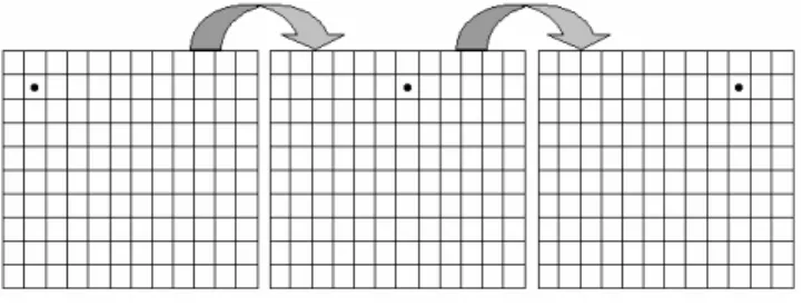
Cruz et al. (1999) proposed the simulation of a single well, which was positioned sequentially in each cell of the grid. Usually, the number of simulations would be very high to test every cell of the grid so selected positions can be evaluated as shown in Fig. 1. The other grid cells quality index can be interpolated. A higher number of block tests yields a better precision, especially for heterogeneous reservoirs.
Figure 1. Well position variation.
Groups of Vertical Wells
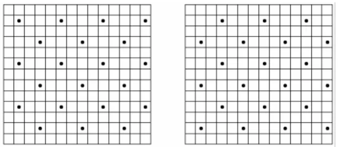
Figure 2. Distribution of vertical wells in 2 groups to build quality map.
All wells belonging to a group are opened at the same time, however, different groups are simulated separately; in both cases production time is set in order to drain as much oil as possible. When working with a single group, the reservoir pressure is reduced faster than with two or more groups, therefore the total simulation time is shorter. When simulating different groups, the results are combined to achieve a solution that is valid for the whole reservoir.
Generating quality maps by simulating horizontal wells is similar to the process using vertical ones, except for the fact that horizontal wells are drilled through single layers. Therefore, the steps described here must be repeated for each layer and then an average is calculated to acquire a final, 2D representation of the reservoir.
The case with a single, horizontal well was not tested since it presents basically the same problem of single, vertical wells, which is the large number of simulations required, this time multiplied by the number of reservoir layers.
Groups of Horizontal Wells
A procedure to generate quality maps using horizontal wells was tested in this work; the wells were placed evenly throughout one layer of the reservoir and simulation took place; the wells distribution can be seen in Fig. 3, for one layer.
Figure 3. Distribution of horizontal wells in 1 group to build quality map.
There are other possibilities to generate the quality map using numerical simulation. Basically, it can be observed the precision increases as the number of simulations increases because more tests are performed guaranteeing a better resolution of the map and a better definition of the influence of each well in the reservoir. The generation of quality maps using injectors are also possible but this technique was not used so far. In this work 2-dimensional maps are used; 3-dimensional maps can be generated using the same procedure but they would increase the computational time; this
could be necessary when working with reservoirs presenting great variations in the vertical permeability, that is, with a high degree of heterogeneity in the vertical direction, however, in several cases the generation of 3D quality maps would bring no significant improvements to the process compared to 2-dimensional ones.
Generation of Quality Maps by Analytical Methods
As an attempt to speedup the process, analytical methods can be used. However, this approach is not recommended for reservoirs with strong heterogeneities. The method studied here was based on the work of Babu and Odeh (1989), who considered a uniform flux solution. In this method, the “quality” was taken as the production rate of a well positioned in a specific location and was given by the following equation (Nakajima and Schiozer, 2003):
+ − + µ − × = − R H w wf r z x S C r A B p p k k b q 75 . 0 ) ln( / ln ) ( 10 08 . 7 2 1 3 (1) where
[
(1/3) ( / ) ( / )]
lnsin(
180 /)
0.5ln 1.088 28. 6 )
ln( 0 0 2 0 −
− − + − = x z o x z H k k h a h z a x a x k k h a
C (2)
Different well locations are set so that the entire reservoir can be analysed thus the map can be built. Some variables must be defined prior to the calculations, namely the horizontal area of drainage (typically, a box surrounding the well), the thickness of the drainage volume and the properties of the drainage volume. Both the thickness and the properties are averaged values considering all the layers and all the drainage cells.
Generation of Quality Maps by Fuzzy Logic
The previous methods are somewhat similar, considering that they basically integrate a series of variables affecting well productivity and provide a single output parameter, used as a “quality index”. This third method offers a different approach to the same problem; fuzzy logic systems do not require computational models or mathematical equations to establish a relationship between input and output parameters. Such a relationship is set via simple rules defined by a knowledge basis. Therefore, to generate a quality map it was necessary to build the fuzzy system, using some of the variables which influenced most the productivity of horizontal wells: porosity, net to gross ratio, oil saturation, vertical and horizontal permeability values, distances of well to aquifer and to gas cap; these variables were chosen based on sensitivity analysis and literature review. The classification applied to the parameters to build the fuzzy system is shown in Table 1.
Table 1. Input parameters for fuzzy system.
Porosity Net to gross ratio
0.2-1.0 High 0.6-1.0 High
0.1-0.2 Medium 0.3-0.6 Medium
0-0.1 Low 0-0.3 Low
Horizontal permeability (mD) Vertical permeability (mD)
1500+ High 300+ High
300-1500 Medium 100-300 Medium
0-300 Low 0-100 Low
Distance to aquifer (m) Distance to gas cap (m)
30+ High 30+ High
10-30 Medium 10-30 Medium
0-10 Low 0-10 Low
Oil saturation
A set of fuzzy rules was determined by simulating a reservoir with all the possible combinations of the values shown in Table 1. These simulations involved a 36x36x7 grid with a single well at the centre, used to determine the oil production. Once the fuzzy system is configured, new maps can be generated by providing the parameter values for each grid cell; the system will then return a value between 0 (zero) and 1 (one), which is the quality index.
Quality Maps – Application
The model studied was derived from a real reservoir, with some alterations made to its permeability: high horizontal permeability channels were added, as can be seen in Fig. 4.
Figure 4. Reservoir model with horizontal permeability channels.
Different methods for building quality maps will yield somewhat different maps; Table 2 shows a comparison of some methods (Nakajima and Schiozer, 2003; Nakajima, 2003); it can be seen that the best method (highest correlation factor) was the numerical simulation using a single well; it took many more simulations than the others, though, and this could be a restricting factor depending on the size of the reservoir. The fuzzy logic system, on the other hand, needs no simulation once the system is built because the fuzzy rules are set in a generalised form and it has presented a good correlation factor. Therefore, the fuzzy logic system was chosen in this work.
Table 2. Comparing methods for building quality maps.
Method Number of
simulation runs
Correlation factor (R2) Simulation of a group of horizontal
wells 1 0.1395
Simulation of a group of vertical wells 1 0.846
Simulation of 2 groups of vertical wells 2 0.8152
Simulation of 4 groups of vertical wells 4 0.7849
Simulation of a single vertical well 58 0.8963
Fuzzy logic system* --- 0.865
Analytical --- 0.7808
* previous simulations are necessary to generate the system
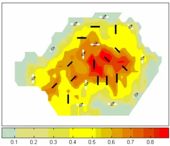
A comparison between two strategies of production for the reservoir depicted above was performed; both strategies involved the use of 14 producer wells and 12 injectors. In strategy number 1, they were allocated in a 5-spot configuration, whereas in strategy number 2, a quality map was used to allocate the producer wells, as shown in Fig. 5; the producers were located in areas of medium to high quality factors, while the injectors were distributed according to the producers distribution and the need to increase pressure in specific regions of the field (which is why some injectors can be seen in areas of high quality indexes).
Figure 5. Initial strategy. Producer wells are black, injectors are white.
As can be seen from Fig. 6, the strategy based on the quality map yielded better results, with higher values of net present value and cumulative oil production. This difference could be even bigger when larger reservoirs are considered, due to the high number of wells used in these fields.
Case VPL (MM US$) Np (MM m3) Wp (MM m3) Gp (MM m3)
Without Map 762 45 41 5349
Using Map 878 46 22 5598
Variation +15% +2% -46% +5%
Figure 6. Comparing Strategies 1 and 2.
Strategy Optimisation
Projects of reservoir recovery can be divided into two basic stages, when considering a new field: the first phase, also called “strategy choice”, where one defines important parameters associated to recovery strategies, e.g. well types and geometry; this and other evaluations can be undertaken either manually or as part of an automatic methodology, as proposed by Mezzomo and Schiozer (2003). The second phase, named “strategy definition”, consists of optimising the choices made in the first stage, which involves the minimization (or maximization) of an objective function, e.g., the net present value, oil, water and gas cumulative production, or even a combination of these parameters. This phase is where the work presented here is situated.
Three optimisation processes were analysed, in order to evaluate the usefulness of quality maps:
Process 1: the quality map was not used; initial strategy based on a 5-spot wells configuration.
Process 2: the quality map was used only to define the initial strategy; for such a task, the map was built at the initial time (i.e., using the properties at the beginning of the simulation) and it was used to define the initial location of the wells; for the remaining of the optimisation, the five parameters described above were used.
Process 3: the quality map was used during the whole optimisation process; the map was generated at the beginning of the simulation, however, its quality index values were used to help in the definition of the classification regions during the optimisation, as described previously.
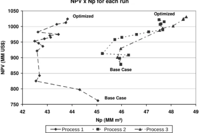
The quality maps actually made it possible to obtain better results with a lower number of simulations, as can be seen in Fig. 7. The relationship between NPV and the cumulative production of oil is more direct in process 3, indicating that the improvement in the income was due to higher oil production, whereas the relationship displayed in process 1 implies that the higher income was a result of cost cuts (reduction of water production or investments). In process 1, the wells presenting bad performance were simply removed from the simulations, resulting in the increase in NPV accompanied by a decrease in Np. When using the quality map, however, it was possible to determine if the region surrounding such wells had potential for better production, in which case attempts to recover those wells (=improve their production) looked favourable. Fig. 7 also shows that using the map only at the beginning of the simulation should yield better results, but adopting the map index as an additional parameter during the process results in a more straightforward path to the desired goal, since it shows the reservoir characteristics with regard to the potential of production.
As production optimisation is a subjective task, the strategy referring to process 1 could eventually reach the final point of process 2 or 3, however it would take many more simulations and, therefore, time, than when working with the assistance of these maps.
NPV x Np for each run
750 800 850 900 950 1000 1050
42 43 44 45 46 47 48 49
Np (MM m³)
N
P
V
(
M
M
U
S
$
)
Process 1 Process 2 Process 3
Base Case Base Case
Optimized Optimized
Figure 7. Evolution of optimisation processes: influence of map quality.
Table 3 shows some more information about the processes. The third process resulted in higher NPV and Np values, taking considerably less simulations to achieve such results. Although optimisation is a subjective process, the quality map has shown itself to be quite useful in the cases studied here; it helped in the
decision making stage and in the wells reallocation, leading to more secure and correct actions.
Table 3. Comparing process data.
Process 1 Process 2 Process 3 NPV (US$ millions) 1024 1021 1031 Np (106 m3) 43.8 47.5 48.6 Total number of runs 33 25 18
Concluding Remarks
Quality maps are powerful visualisation tools that can combine several parameters characteristic of the reservoir under analysis and yield a final index, which can serve as an invaluable tool for the optimisation of production strategies. Well allocation is a complex task which can require a relatively long time in the analysis of the reservoir characteristics. These maps can assist in the determination of the best regions to place a producer well, resulting in a better starting point.
During optimisation of production strategies, one could conclude, by simply analysing productivity profiles, that the best way to deal with poorly performing wells would be to remove them from the simulation; quality maps can, in these situations, define if the well should be excluded or recovered, by providing insight into the potential for production of the area of the well: if it is located in a region with good potential, the well could be recovered, whereas attempts to recover wells located in bad regions would only lead to waste of simulations and time. This tool can, therefore, help with improving the efficiency of the optimisation process by eliminating future steps and leading a more direct path towards the desired goal.
The methods for building quality maps shown here represent approximate solutions, due to the simplifications done during the process; they can, however, evolve to higher accuracy solutions as the reservoir is evaluated during the optimisation.
Acknowledgements
The authors are grateful to CNPq, Petrobras and FINEP/CTPETRO for their financial support to this project, and to José Sérgio de A. Cavalcante Filho for his assistance with the quality map figure.
References
Babu, D.K. e Odeh, A.Z., 1989, “Productivity of a Horizontal Well”; SPE Reservoir Engineering, Vol.4, No.4, pp. 417-421. SPE 18298.
Bittencourt, A.C. and Horne, R.N., 1997, “Reservoir Development and Design Optimization”. In: SPE Annual Technical Conference and Exhibition, San Antonio, Texas, USA, October 5-8, SPE 38895.
Cruz, P.S., Horne, R.N. and Deutsch, C.V., 1999, “The Quality Map: a Tool for Reservoir Uncertainty Quantification and Decision Making”. In: SPE Annual Technical Conference and Exhibition, Houston, Texas, USA, October 3-6, SPE 56578.
Cruz, P.S., 2000, “Reservoir Management Decision-Making In The Presence Of Geological Uncertainty”. Stanford, USA. 239p. PhD – Department of Petroleum Engineering, Stanford University.
Güyagüler, B., Horne, R.N., Rogers, L. and Rosenzweig, J.J., 2002, “Optimization of Well Placement in a Gulf of Mexico Waterflooding Project”. SPE Reservoir Evaluation and Engineering, Vol.5, No.3, pp. 229-236, SPE 78266.
Guyaguler, B. and Horne, R., 2000, “Optimization of Well Placement”. Journal of Energy Resources Technology – Transactions of the ASME, Vol. 122, No. 2, pp. 64-70.
Mezzomo, C.C. and Schiozer, D.J., 2003, “Methodology for Water Injection Strategies Planning Optimization Using Reservoir Simulation”. Journal of Canadian Petroleum Technology, Vol. 42, No. 7, pp. 9-11.
Montes, G., Bartolome, P. and Udias, A.L., 2001, “The Use of Genetic Algorithms in Well Placement Optimization”. In: SPE Latin American and Caribbean Petroleum Engineering Conference, Buenos Aires, Argentina, March 25-28, SPE 69439.
Nakajima, L., 2003, “Horizontal Wells Performance Optimization on Petroleum Fields Development”. Campinas, Brazil. 147p. MSc. – School of Mechanical Engineering and Institute of Geosciences, UNICAMP. (In Portuguese).
Nakajima, L. and Schiozer, D.J., 2003, “Horizontal Well Placement Optimization Using Quality Map Definition”. In: 2003 Petroleum Society’s
Canadian International Petroleum Conference, Calgary, Alberta, Canada, CIPC 2003-053, June 10-12.
Raghuraman, B., Couet, B. and Savundararaj, P., 2003, “Valuation of Technology and Information for Reservoir Risk Management”. SPE Reservoir Evaluation and Engineering, Vol. 6, No. 5, pp. 307-315.
Wagenhofer, T. and Hatzignatiou, D.G., 1996, “Optimization of Horizontal Well Placement”. In: Western Regional Meeting, Anchorage, Alaska, USA, May 22-24, SPE 35714.