Variability of aerosols forecast over the Mediterranean area during July 2013 (ADRIMED/CHARMEX)

(1)

ACPD

15, 10341–10388, 2015

Variability of aerosols forecast during

CHARMEX

L. Menut et al.

Title Page

Abstract Introduction

Conclusions References

Tables Figures

◭ ◮

Back Close

Full Screen / Esc

Printer-friendly Version Interactive Discussion

Discussion

P

a

per

|

Discussion

P

a

per

|

Discussion

P

a

per

|

Discussion

P

a

per

|

Atmos. Chem. Phys. Discuss., 15, 10341–10388, 2015 www.atmos-chem-phys-discuss.net/15/10341/2015/ doi:10.5194/acpd-15-10341-2015

This discussion paper is/has been under review for the journal Atmospheric Chemistry and Physics (ACP). Please refer to the corresponding final paper in ACP if available.

Variability of aerosols forecast over the

Mediterranean area during July 2013

(ADRIMED/CHARMEX)

L. Menut, G. Réa, S. Mailler, D. Khvorostyanov, and S. Turquety

Laboratoire de Météorologie Dynamique, UMR CNRS 8539, Ecole Polytechnique, Ecole Normale Supérieure, Université P. M. Curie, Ecole Nationale des Ponts et Chaussées, Palaiseau, France

Received: 21 January 2015 – Accepted: 20 March 2015 – Published: 9 April 2015

Correspondence to: L. Menut (menut@lmd.polytechnique.fr)

(2)

ACPD

15, 10341–10388, 2015

CHARMEX

L. Menut et al.

Title Page

Tables Figures

◭ ◮

Back Close

Full Screen / Esc

Discussion

P

a

per

|

Discussion

P

a

per

|

Discussion

P

a

per

|

Discussion

P

a

per

|

Abstract

The atmospheric composition was extensively studied in the Euro-Mediterranean re-gion and during the summer 2013, in the framework of the ADRIMED project. During the campaign experiment, the WRF and CHIMERE models were used in forecast mode in order to help scientists to decide whether Intensive Observation Periods should be

5

triggered or not. Each day, a simulation of four days is performed, corresponding to

leads from (D₋1) to (D₊2). The goal of this study is to know the reason why the

model does not always simulate in advance what is finally observed: is it due to sys-tematic biases in the models used or to a too large variability due to the real non-linear nature of the meteorology and chemistry? To answer this question, the methodology

10

is to compare the several modelled forecast leads to observations. It was shown that

the differences between observations and model is always higher than between the

forecast leads. If chemistry-transport model results are not close to the observations, this is mainly due to the model itself (including the meteorology) and its biases. But the forecast variability also acts a lot, mainly due to the modelled wind. This variable

15

is at the origin of the mineral dust and sea salt emissions, as well as the long-range transport of these long-lived species: the wind bias combined to its variability is at the origin of the major part of the aerosols forecast errors.

1 Introduction

The regional air quality was originally focussed on photochemical pollution such as

20

ozone and nitrogen dioxides (Fenger, 2009). This interest was partly motivated by the european “air directives” of 1996, establishing contraints to reduce air pollution for gaseous species only (Monks et al., 2009). More recently, the need of a better understanding of aerosols was added in this regulation framework. If the particulate

matter with a diameter less than 10 µm (called PM₁₀) is controlled since many years,

25

(3)

ACPD

15, 10341–10388, 2015

CHARMEX

L. Menut et al.

Title Page

Tables Figures

◭ ◮

Back Close

Full Screen / Esc

Discussion

P

a

per

|

Discussion

P

a

per

|

Discussion

P

a

per

|

Discussion

P

a

per

|

addition of PM_2.5routinely measurements (European Union, 2008). In this context, the

Mediterranean is well known as an hot spot for this high aerosols concentrations as well as high spatial and temporal variability (Millan et al., 2005).

Aerosols sources and sinks studies remain difficult since a lot of different compo-nents are included in these particulate matters: several chemical species or materials

5

(organic matter, sulfates, nitrates, ammonium, mineral dust, sea salt etc.), with several sizes and shapes, several origins in space, lifetimes, potential direct and indirect ef-fects on radiation, cloud formations, etc. In order to reduce potential damages due to too high aerosols concentrations, it is thus necessary to improve our knowledge on all these aspects (Carslaw et al., 2010).

10

A way to reduce atmospheric pollution is to accurately forecast atmospheric con-centrations in order to be able to act at the right time and place to reduce the anthro-pogenic part of the emissions. This remains today a challenge and forecast systems often miss large pollution events. Some previous studies tried to identify and thus re-duce the forecast error. For example, Manders et al. (2009) quantified the capability of

15

the LOTOS-EUROS system to forecast PM10. By reducing some systematic identified

biases, Borrego et al. (2011) showed the forecast could be improved over Portugal. An-other way to improve forecast is to reduce biases by increasing realism in the aerosols

representation: this was conducted in Mulcahy et al. (2014) for the Met Office global

numerical weather prediction model, showing a benefit on the forecast scores. More

20

recently, several studies showed that data assimilation may reduce the forecast er-ror by constraining the forecast initial conditions, as in Niu et al. (2008) and Curier et al. (2012). For all these studies, bias and variability were treated together. Other framweorks provide daily experimental forecast such as DREAM (Pérez et al., 2007) and SKYRON (Spyrou et al., 2013) but they mainly focussed on mineral dust.

25

In the present study, we propose to estimate the relative contributions of two mod-elling aspects, the bias and the variability, by comparing several forecast leads to

ob-servations. The main question isto what extent the differences between observed and

(4)

ACPD

15, 10341–10388, 2015

CHARMEX

L. Menut et al.

Title Page

Tables Figures

◭ ◮

Back Close

Full Screen / Esc

Discussion

P

a

per

|

Discussion

P

a

per

|

Discussion

P

a

per

|

Discussion

P

a

per

|

of the atmospheric system to represent?To answer this question, we take advantage of the CHARMEX program (Dulac et al., 2013), and more precisely to the ADRIMED project, studying the atmospheric composition during June and July 2013 and over the Mediterranean area (Mallet, 2015). During the months of June and July 2013, the ADRIMED project experimental part was conducted to document the atmospheric

com-5

position in the Western-Mediterranean region. In parallel to these measurements, re-gional models were used in real-time forecast to help the instrumental teams to define when and where the best measurements can be done. In this case, the models are not used to analyze the meteorology and chemical composition during a long period but only to quickly provide informations about the current state of the atmosphere and its

10

probable evolution during the next days.

The present study was done using the same measurements and models configura-tions than the ones presented in Menut et al. (2015). The added value in the present study is the use of this modelling plat-form in a forecast mode. Section 2 summarizes the sites from where observations are used. Section 3 presents the modelling system

15

and the forecast set-up. Sections 4 and 5 present the variability of the forecasted me-teorological fields and pollutants emissions, respectively. Section 7 presents aerosols concentrations results and their variability as maps and for selected sites using time se-ries and vertical profiles, compared to the available measurements. Conclusions and perspectives are presented in Sect. 8.

20

2 The observations

In this study, the observations used are the same as those used in Menut et al. (2015): the AERONET hourly measurements (Dubovik and King, 2000), for the Aerosol Optical

Depth (AOD) and the EEA network data (Guerreiro et al., 2013), for the surface PM10

concentrations. All the measurements sites locations used in this study are

summa-25

(5)

ACPD

15, 10341–10388, 2015

CHARMEX

L. Menut et al.

Title Page

Tables Figures

◭ ◮

Back Close

Full Screen / Esc

Discussion

P

a

per

|

Discussion

P

a

per

|

Discussion

P

a

per

|

Discussion

P

a

per

|

are presented. In addition, specific measurements performed during the ADRIMED campaign and located at Lampedusa and Cape Corsica are added to the analysis.

3 The modeling system

The modeling system is composed of several models: the WRF regional meteorological model, the CHIMERE chemistry-transport model and additional individual models for

5

emissions fluxes estimations. All these models are integrated in a modelling plat-form usable both in analysis and forecast mode. We first describe the whole modelling plat-form, including the forecast configuration, then the models WRF and CHIMERE. This modelling plat-form is strictly the same than the one extensively described in Menut et al. (2015).

10

3.1 The forecast configuration

Even if the WRF and CHIMERE models have regurlarly new versions, the forecast con-figuration of these models remains the same and was previously used in many studies as listed in (Menut and Bessagnet, 2010). More precisely, this forecast configuration was used during the ESCOMPTE project in the south of France (Menut et al., 2005) and

15

during the AMMA experimental campaign for mineral dust aerosols in western Africa (Menut et al., 2009). CHIMERE is also used in an operational context since 2003 for the PREVAIR French air quality forecast (Honoré et al., 2008; Rouïl et al., 2009), and in the MACC European project (Inness et al., 2013).

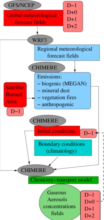
This forecast system is presented in Fig. 1. The first step is to calculate forecasted

20

regional meteorology. The global GFS/NCEP forecast fields are used to force the

re-gional WRF3.5.1 model (see detailed description below) and from (D₋_{1) (i.e. the day}

before) to (D₊2) (two days in advance). They are then used for several calculations:

(i) the surface emissions fluxes, (ii) the transport and mixing of gaseous and aerosols species with CHIMERE. For the specific case of the vegetation fires emissions, satellite

(6)

ACPD

15, 10341–10388, 2015

CHARMEX

L. Menut et al.

Title Page

Tables Figures

◭ ◮

Back Close

Full Screen / Esc

Discussion

P

a

per

|

Discussion

P

a

per

|

Discussion

P

a

per

|

Discussion

P

a

per

|

observations of fire activity (MODIS near-real time detection) during the previous day are analyzed to derive the corresponding area burned. These are then used as input to the high resolution fire emissions model (Turquety et al., 2014), assuming fires will continue burning during the first 72 h of the forecast period. The biogenic and mineral dust emissions fluxes depend on the meteorology, when the anthropogenic emissions

5

are only dependent on the week day. The initial conditions for gas and aerosols con-centrations are taken from the forecast of the day before. In practice, this means that the system was launched several days before the first day for the first forecast of the period and in order to have a correct spin-up.

In this study, the simulation was performed from 10 June to 5 July 2013. Each day,

10

a simulation of four days is performed, from (D₋1) to (D₊2). For each modelled pe-riod, meteorological parameters, gas and aerosols species are hourly calculated on the domain grid. Thus, for each of these parameters, each grid cell and each hour of

the period, this allows to have four di_fferent values. By comparing these four values,

we can quantify the forecast variability. For the results analysis, the focus will be done

15

on the period ranging from the 14 to the 26 June 2013, identified as the period with the most interesting pollution events during the ADRIMED project.

3.2 The meteorological model WRF

The meteorological parameters are modelled with the WRF regional model in its ver-sion 3.5.1. The model is used in its non-hydrostatic configuration, with a constant

hor-20

izontal resolution of 60 km×60 km and 28 vertical levels from surface to 50 hPa. The

Single Moment-5 class microphysics scheme is used allowing for mixed phase pro-cesses and super cooled water (Hong et al., 2004). The radiation scheme is RRTMG scheme with the MCICA method of random cloud overlap (Mlawer et al., 1997). The surface layer scheme is based on Monin-Obukhov with Carslon-Boland viscous

sub-25

(7)

ACPD

15, 10341–10388, 2015

CHARMEX

L. Menut et al.

Title Page

Tables Figures

◭ ◮

Back Close

Full Screen / Esc

Discussion

P

a

per

|

Discussion

P

a

per

|

Discussion

P

a

per

|

Discussion

P

a

per

|

et al., 2006) and the cumulus parameterization uses the ensemble scheme of Grell and Devenyi (2002).

The global fields of NCEP/GFS are hourly read by WRF using nudging techniques and for the main atmospheric variables (pressure, temperature, humidity, wind). In or-der to preserve both large-scale circulations and small scale gradients and variability,

5

the “spectral nudging” was chosen. This nudging was evaluated in regional models, as presented in Von Storch et al. (2000). In this study, the spectral nudging was selected

to be applied for all wavelength greater than≈2000 km (wavenumbers less than 3 in

latitude and longitude, for wind, temperature and humidity and only above 850 hPa). This configuration allows the regional model to create its own structures within the

10

boundary layer but to follow the large scale meteorological fields.

3.3 The chemistry-transport model CHIMERE

CHIMERE is a chemistry-transport model able to simulate concentrations fields of

gaseous and aerosols species at a regional scale. The model is off-line and thus

needs pre-calculated meteorological fields to run. In this study, we used the version

15

fully described in Menut et al. (2013a). The horizontal domain is the same as the one of WRF. For the vertical grid, the 28 vertical levels are projected onto the 20 levels of the CHIMERE mesh.

The gaseous species are calculated using the MELCHIOR 2 scheme and the aerosols using the scheme developed by Bessagnet et al. (2004). This module takes

20

into account species such as sulphate, nitrate, ammonium, primary organic (OC) and black carbon (BC), secondary organic aerosols (SOA), sea salt, dust and water. These aerosols are represented using nine bins, from 40 nm to 20 µm, in diameter. The life cycle of these aerosols is completely represented with nucleation of sulphuric acid, co-agulation, adsorption/desorption, wet and dry deposition and scavenging. This

scav-25

(8)

ACPD

15, 10341–10388, 2015

CHARMEX

L. Menut et al.

Title Page

Tables Figures

◭ ◮

Back Close

Full Screen / Esc

Discussion

P

a

per

|

Discussion

P

a

per

|

Discussion

P

a

per

|

Discussion

P

a

per

|

The anthropogenic emissions are estimated using the same methodology as the one described in Menut et al. (2012) but with the HTAP masses as input data. These masses were prepared by the EDGAR Team, using inventories based on MICS-Asia, EPA-US/Canada and TNO databases (http://edgar.jrc.ec.europa.eu/htap_

v2/index.php?SECURE=123). Biogenic emissions are calculated using the MEGAN

5

emissions scheme (Guenther et al., 2006) which provides fluxes of isoprene, terpene and pinenes. In addition to this version, several processes were improved and added in the framework of this study. First, the mineral dust emissions are now calculated using new soil and surface databases, as described in Menut et al. (2013b). Second, chemical species emissions fluxes produced by vegetation fires are estimated using

10

the new high resolution fire model presented in Turquety et al. (2014). And, finally, the photolysis rates are explicitely calculated using the FastJ radiation module, (Wild et al., 2000) and as fully described in Mailler et al. (2015).

4 Predictability of meteorological parameters

Due to many processes, the atmospheric concentrations of trace gases and aerosols

15

are very sensitive to the meteorological fields. First, some of the sources are directly dependent on the near-surface meteorology: (i) the mineral dust emissions depend on the surface wind speed, (ii) the biogenic emissions depend on temperature and radia-tion, and (iii) the fires emissions depend on the soil moisture (for fire efficiency) and the boundary layer dynamics (for the pyroconvection). Second, during the transport, the

20

atmospheric species will be under the influence of: (i) the wind, pressure, humidity and temperature for the boundary layer dynamics and tropospheric long-range transport and (ii) the clouds and radiation attenuation for the photochemistry. Finally, the sinks of atmospheric species are mainly (i) the surface layer turbulence acting on gas and aerosols dry deposition and, (ii) the precipitations by the way of aerosols scavenging. In

25

(9)

ACPD

15, 10341–10388, 2015

CHARMEX

L. Menut et al.

Title Page

Tables Figures

◭ ◮

Back Close

Full Screen / Esc

Discussion

P

a

per

|

Discussion

P

a

per

|

Discussion

P

a

per

|

Discussion

P

a

per

|

4.1 Variability of 2 m temperature

The variability of the 2 m temperature is studied using statistical scores and direct inter-pretation of time series for selected sites. The modelled 2 m temperatures are extracted for two kind of locations. First, European stations where E-OBS data are available (listed in Table 2). In this case, comparisons to the measurements are presented.

Sec-5

ond, the three sites of Banizoumbou, Cape Corsica and Lampedusa, being of interest for other dependent variables as the mineral dust, sea salt and biogenic emissions. In this case, comparisons are done between the modelled results only in order to quantify the variability of the model between the several forecast leads.

4.1.1 Statistical scores for 2 m temperature

10

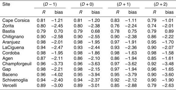
Table 2 present scores for the comparison between the E-OBS data and the corre-sponding model values. The several forecast leads are compared to the observations

using correlationR _{and absolute bias. In general, the correlations between}

measure-ments and modelled values are always good with values higher than 0.74. The bias

is mainly negative with values between 0.7 (Bastia) to−4.02 K (Champforgeuil) for the

15

(D₋_{1) simulation. This shows, in general, that the model underestimates the mean}

daily 2 m temperature over the whole simulation domain.

The correlation values decrease when the forecast lead increases: this is a logical result, the uncertainty growing with the forecast lead. For example, the correlations ranges from 0.81 to 0.79 in Cape Corsica, 0.96 to 0.90 in Baceno, 0.89 to 0.79 in

20

(10)

ACPD

15, 10341–10388, 2015

CHARMEX

L. Menut et al.

Title Page

Tables Figures

◭ ◮

Back Close

Full Screen / Esc

Discussion

P

a

per

|

Discussion

P

a

per

|

Discussion

P

a

per

|

Discussion

P

a

per

|

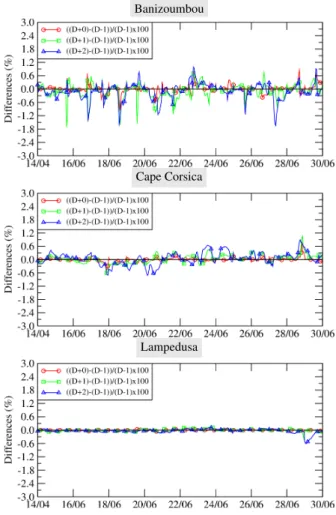
4.1.2 Time series of 2 m temperature

Time series of observed and modelled daily mean averaged 2 m temperature are dis-played in Fig. 2. These time series are presented as examples of the results discussed before and are for the Zorita (Spain), Agen (France) and Vercelli (Italy) sites. The sys-tematic model underestimation clearly appears. But, over the whole period, the model

5

shows its ability to model the weekly variability i.e. is able to reproduce the main synop-tic circulations: this is certainly the most important point for the modelling of emissions and long-range transport of pollutants over this large region including North of Africa and Europe.

Figure 2 shows that the variability between the forecast leads is lower than the diff

er-10

ences between the observations and the model. In order to better see the differences

between the forecast 2 m temperature time-series, Fig. 3 presents the percentages of differences between the forecast (D₊0), (D₊1), (D₊2) and the “analysis” fields, (D_−1).

These figures, (unlike the daily mean of Fig. 2), are here with hourly values of the 2 m temperature in order to see the hourly variability.

15

Three sites are chosen for this comparison and they were selected as sites

repre-sentative of very different locations in the domain: Banizoumbou, Cape Corsica and

Lampedusa. These are also sites where E-OBS data are not available, being in Africa and over islands in the Meditteranean. Note that these percentages are calculated

using temperature values in Kelvin. The maximum differences are calculated for

Ban-20

izoumbou: over the whole period, values range from ≈ −2 to +2 % (i.e. for a mean

value of 300 K, a variability of ±6 K). In Cape Corsica, the maximum differences are

lower and≈ −0.5 to+0.5 %. Finally, in Lampedusa, the differences may be considered

as negligible with values less than 0.2 % (i.e. less than 0.6 K).

4.2 Variability of the wind speed and direction

25

(11)

ACPD

15, 10341–10388, 2015

CHARMEX

L. Menut et al.

Title Page

Tables Figures

◭ ◮

Back Close

Full Screen / Esc

Discussion

P

a

per

|

Discussion

P

a

per

|

Discussion

P

a

per

|

Discussion

P

a

per

|

the mineral dust and sea salt emissions as well as the diurnal cycle of the convection in the boundary layer. In altitude, horizontal transport is constrained by this variable. In order to quantify the wind variability, several forecast leads are first compared in terms of 10 m wind speed times series. Second, vertical profiles are compared. Note that for these two comparisons, there are no measurements available.

5

4.2.1 Time series of 10 m wind speed

The 10 m wind speed,|U_|_{10 m}_{, is an important parameter for numerous processes a}_ff

ect-ing the atmospheric composition: its value is directly used in many model parameteri-zations as the saltation and sandblasting processes, driving the mineral dust emission fluxes. This is also a key parameter for the estimation of dry deposition velocities. Close

10

to the surface, the wind speed varies a lot naturally, depending on the atmospheric sta-bility as well as the horizontal heteorogeneity of the studied location.

The variability of |U_|_{10 m} _{is quantified, for comparison, at the same sites as those}

used for the 2 m temperature. Results are displayed in Fig. 4 for these sites with the modelled absolute values on the left panel and the variability on the right panel. This

15

variability is expressed as a percentage of differences between the (D_{−1) forecast and}

the other forecasts (D₊_0,D₊_{1 and}D₊_{2). In order to avoid unrealistic values due to}

wind speed close to zero, the calculations of the percentages are done only for values |U_|₍_D₋₁₎>_{0.1 m s}−1_.

Compared to the 2 m temperature, the 10 m wind speed variability is very high. There

20

is no specific systematic bias and the values of di_fferences ranged from 0 to 250 %,

for wind speed between 0.1 and 10 m s−1. For the site of Banizoumbou, mineral dust

emissions will be sensitive to this wind speed and its variability. It is known that

salta-tion occurs for wind speed values up to ≈6 m s−1 (even if this absolute value may

depend on the soil texture and the landuse). A variability of±1 m s−1(low in absolute

25

(12)

ACPD

15, 10341–10388, 2015

CHARMEX

L. Menut et al.

Title Page

Tables Figures

◭ ◮

Back Close

Full Screen / Esc

Discussion

P

a

per

|

Discussion

P

a

per

|

Discussion

P

a

per

|

Discussion

P

a

per

|

one of the most sensitive parameters. Values of variability are more moderate than in Banizoumbou but still very high: with values up to 150 % in Cape Corsica and 130 % in Lampedusa.

4.2.2 Vertical profiles of wind speed and direction

Figure 5 presents vertical profiles of mean wind speed and wind direction for two

loca-5

tions corresponding to the Cape Corsica and Lampedusa ADRIMED super-sites. The profiles are presented for the whole atmospheric column modelled by CHIMERE, from the surface to 8000 m a.g.l. and for the 18 and 21 June 2013 at 12:00 UTC.

For the 18 June, the wind speed is lower than for the 21 June over the two sites. For

the two sites and the two days, the values are close between (D₋_{1) and (}D₊_{0). On}

10

the contrary, large differences appear between (D₋1) and the forecasts at (D₊1) and

(D₊_{2). For example, on 18 June at Cape Corsica, in the lower troposphere, the wind}

speed is lower than 6 m s−1for (D₊_{1) and (}D₊_{2), while the values are around 8 m s}−1

for (D_{−1) and (}D₊0). In this case, the forecasted transport is lower and may induce air masses being not transported at the right time in this area. On the contrary, while the

15

modelled wind speed seems to have a low variability and low values for (D₋_{1), (}D₊₀₎

and (D₊_{1) in Lampedusa and for 21 June, the (}D₊_{2) forecast shows larger values:}

for an altitude around 3000 m a.g.l., the wind speed varies from 2 to 10 m s−1. In this latter case, the forecasted aerosol plumes could be advected too fast in the middle of the Mediterranean.

20

The wind direction also exhibits a large variability. For long-range transport of aerosol plumes, the largest variability is modelled in Lampedusa for the 18 and 21 June and for altitudes between 2000 and 4000 m. For the other sites and days, the wind direction variability is smaller in the low troposphere. In altitude, a very strong forecast variability is modelled in Cape Corsica, for the 18 June: but this variability is up to 6000 m, and

25

(13)

ACPD

15, 10341–10388, 2015

CHARMEX

L. Menut et al.

Title Page

Tables Figures

◭ ◮

Back Close

Full Screen / Esc

Discussion

P

a

per

|

Discussion

P

a

per

|

Discussion

P

a

per

|

Discussion

P

a

per

|

4.3 Variability of precipitations

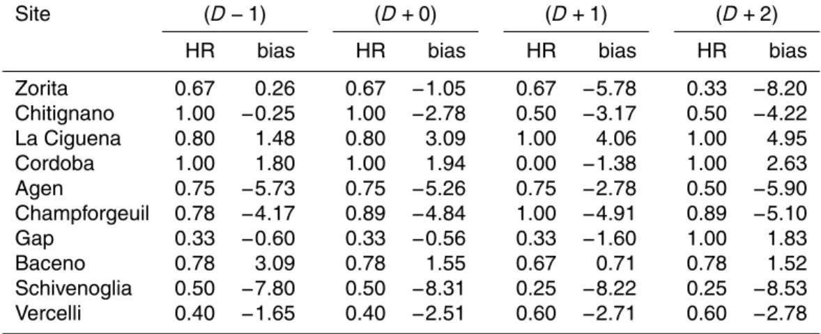
Results of Hit Rates and biases between the E-OBS observations and modelled values are presented in Table 3. The Hit Rates are calculated as described in Menut et al. (2015), for the same period, region and data. Note that the number of studied sites is reduced compared to the 2 m temperature: this is just because no precipitation was

5

recorded for some sites, leading to the impossibility to quantify scores. For the sites where precipitation amount was observed and/or modelled, the results showed that this variable is correctly modelled in time frequency, but less in magnitude. The Hit

Rates vary from 0.33 (in Gap) to 1 for (D₋_{1) compared to the observations. These}

scores are the same or worse for the comparison between the E-OBS observations

10

and the (D₊_{2) simulation, with values ranging between 0.25 to 1. Biases are often}

high: for (D₋_{1), the bias range from}_{−7.80 to}₊_{3.09 mm day}−1_{. From (}D₋_{1) to (}D₊_2),

these bias values logically increase ranging between−8.53 to+4.95.

To quantify the Hit Rates and bias results in terms of magnitude and time, three time series are presented, Fig. 6. Zorita (Spain), Agen (France) and Vercelli (Italy) are

15

considered as representative of the behaviour observed over all stations and were also already presented for the discussion about the 2 m temperature.

In Zorita, three precipitation events are observed during the period: two events are modelled and one missed. For the two modelled events, the model mainly overesti-mate the precipitation amount. The strong bias for this station is mainly due to: (i) the

20

17 June where a precipitation of 11 mm day−1 is observed but not modeleld and (ii)

the 19 June, where the model diagnosed a precipitation that has not been observed. In Agen, five precipitations events are observed, correctly modelled in terms of time period, but less in magnitude. In this case, the model underestimates the observations, leading to a systematic negative bias, as reported in Table 3. At the end of the period,

25

(14)

ACPD

15, 10341–10388, 2015

CHARMEX

L. Menut et al.

Title Page

Tables Figures

◭ ◮

Back Close

Full Screen / Esc

Discussion

P

a

per

|

Discussion

P

a

per

|

Discussion

P

a

per

|

Discussion

P

a

per

|

three precipitation events were observed. They are well modelled for the corresponding days with a moderate underestimation by the model.

Globally, when a precipitation event is observed, it is often reproduced by the model. The precipitation intensity appears more difficult to simulate and a factor of 2 (under-or over-estimation) is often found. A large variability is found between the f(under-orecast

5

lead in terms of magnitude but not in terms of days with or without precipitation. For a chemistry-transport model, independently of the meteorology, the time occurence is more important than the magnitude: the scavenging schemes leading to a global clean-ing of the atmospheric column under a diagnosed precipitatclean-ing cloud. Thus, with these results, it appears that the most sensitive aspect, the time frequency, is sufficiently well

10

modelled, even if the magnitude is certainly not.

5 Predictability of emissions

In this section, the predictability of emissions is quantified for the mineral dust and biogenic emissions. Anthropogenic emissions are not hourly or daily meteorology-dependent and their variability is thus not considered here. For the fire emissions, the

15

model is not able to forecast the burned areas in advance. Each day, the burned areas of the day before are used for the whole period to forecast: the main varying parameter is kept constant. In addition, no significant fire events occurred in June 2013. The fires emission variability is thus not considered too.

5.1 Variability of mineral dust emissions

20

Mineral dust emissions depend on the soil texture, the surface with the landuse and the surface layer wind speed. At the regional scale and during a few days, there is no variability of the soil and surfaces characteristics. On the other hand, the surface layer wind speed can vary a lot. Mineral dust emissions are strongly dependent on the wind speed and, thus, the corresponding friction velocityu_∗ _{(Menut et al., 2013b).}

(15)

ACPD

15, 10341–10388, 2015

CHARMEX

L. Menut et al.

Title Page

Tables Figures

◭ ◮

Back Close

Full Screen / Esc

Discussion

P

a

per

|

Discussion

P

a

per

|

Discussion

P

a

per

|

Discussion

P

a

per

|

These dynamical variables act in a non-linear way: the mineral dust emission occurs only if the friction velocity is greater than a threshold value,uT_∗, itself depending on the surface characteristics. This means that for a small change,ǫ_{, in the friction velocity}

value (parameterized using the 10 m wind speed), the mineral dust emission could be zero (ifu_∗₌uT_∗ ₋ǫ_{) or not (if}u_∗₌uT_∗ ₊ǫ_).

5

Figure 7 presents two maps for the mineral dust fluxes. Even if this model version al-lows the calculation of the mineral dust fluxes over Europe, and with the same scheme as over Africa, the largest fluxes are calculated over Africa. The map for the 20 June 2013 is shown as an example, after daily cumulating the hourly fluxes calculated by the model. For this day, the emissions are mainly over western Africa and Saudi Arabia.

10

Depending on the location, these fluxes range from 0.1 to more than 20 g m−2day−1.

The second map shows the di_fferences between the fluxes calculated for the same

day but at several forecast leads: (D₋_{1) and (}D₊_{2). For the region where the highest}

fluxes are estimated, the absolute differences may be very large i.e. of the same order of magnitude as the flux itself.

15

In order to quantify this variability in a synthetic way, the mineral dust emissions fluxes are daily cumulated over the whole simulation domain. The values are presented in Fig. 8 top and are thus expressed in Tg day−1. These results show that the variability is close between the several leads: the two main peaks are modelled for the 25 and 28 June with the same order of magnitude. These fluxes being mainly wind speed

20

dependent, this means that the model is stable at the synoptic scale and the mean large scales wind variability is reproduced regardless of the forecast lead. Looking in

more detail, some differences are present for each day. For example on 22 June, the

modelled fluxes are relatively low but highly variable.

The same results are expressed in relative differences in Fig. 8 bottom. The sign of

25

these differences is not constant in time, showing a large variability from day to day.

The maximum values of differences are ±30 % of the maximum daily flux. Logically,

the greater the forecast lead (i.e. for (D₊_{1) and (}D₊_{2)), the larger the di}_ff_{erences are}

(16)

ACPD

15, 10341–10388, 2015

CHARMEX

L. Menut et al.

Title Page

Tables Figures

◭ ◮

Back Close

Full Screen / Esc

Discussion

P

a

per

|

Discussion

P

a

per

|

Discussion

P

a

per

|

Discussion

P

a

per

|

Finally, even if the forecast is variable, when a high wind speed is forecasted, this is generally true for all leads: in this case, fluxes occur for all forecast leads. This means that the largest differences are not always for highest fluxes, but can also occur when the wind speed is close to the threshold value.

5.2 Variability of biogenic emissions

5

The biogenic emissions are sensitive to the temperature and the photosynthetic active radiation (PAR). Over vegetative areas, some changes in these meteorological values could impact the isoprene and terpenes emissions fluxes. As for the dust emissions, the biogenic emissions are cumulated over the whole simulation domain. The time series are presented in Fig. 9 top. A moderate day to day variability is modelled over

10

the whole period: starting with a low value of 2.2×109molecules day−1, a maximum of

2.4×109molecules day−1is reached on 17 June, following by a monotonic decrease to

1.8×109molecules day−1.

For all forecast leads, this variability is modelled in the same way. The relative dif-ferences, in %, are displayed in Fig. 9 bottom. For all leads and all days, the same

15

tendency is observed: the greater the forecast lead, the larger the fluxes. But, while

the maximum of variability is between (D₋_{1) and (}D₊_{2), with peaks around} ₊_{6 %,}

these di_fferences are lower for the other days: in average ₊4 % for (D₊1) and₊2 % for (D₊_{0). The overall variability of biogenic emissions is low, with maximum values of}

6 %, consistent with that of the temperature, the latter being its main driver.

20

6 Predictability of aerosols optical depth

(17)

ACPD

15, 10341–10388, 2015

CHARMEX

L. Menut et al.

Title Page

Tables Figures

◭ ◮

Back Close

Full Screen / Esc

Discussion

P

a

per

|

Discussion

P

a

per

|

Discussion

P

a

per

|

Discussion

P

a

per

|

available using satellite data analysis and inversion of photometers data. In this section, the AERONET level 2 data are used.

6.1 Variability of AOD time series

Time series of AOD for selected sites are presented in Fig. 10. The AERONET obser-vations are compared to the four forecast leads from (D₋1) to (D₊2). Hourly values

5

are presented to better explain the large variability of the measurements compared to the modelled values.

In Banizoumbou, the measurements are representative of a site close to the mineral dust sources. Large values of AOD are measured and not modelled. Over the whole period, from 14 to 30 June, two events of large AOD are measured corresponding to

10

the 15 and 21 June. The model is able to reproduce these peaks, but not with the cor-rect timing for the first peak, being modelled on 16 June. For the 21 June peak, only

the (D₊_{1) forecast shows a significant increase of the modelled AOD value. In Capo}

Verde, the available measurements are less numerous. The trend in the observations is reproduced by the model with rather low values between 0.1 and 0.8. A large

vari-15

ability is modelled between the forecast leads, as for the period from 22 to 24 June. In Lampedusa, a site in the middle of the Mediterranean sea and under mineral dust plumes, the main variability over the whole period is well reproduced: the main peak is observed on 24 June and the modelled values are also maximum for this day. The variability between the forecast leads is here moderate.

20

By comparing the observations and the model, it is clear that the forecast

variabil-ity is always lower than the differences between model and observations. In order to

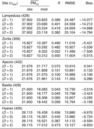
quantify this variability between model and observations, correlation is calculated for each forecast lead and results are presented in Table 4. As well as for time series, calculations are done for hourly values. First, it appears that results are less good than

25

the ones presented in Menut et al. (2015) for the same sites, the same observations

and the same model. The di_fferences between the two studies is the studied period

(18)

ACPD

15, 10341–10388, 2015

CHARMEX

L. Menut et al.

Title Page

Tables Figures

◭ ◮

Back Close

Full Screen / Esc

Discussion

P

a

per

|

Discussion

P

a

per

|

Discussion

P

a

per

|

Discussion

P

a

per

|

15 July 2013, i.e. 45 days. In this study, and since many forecast leads are analyzed, the period reduces to 15 days. This may be explained by the fact that AOD correlations are mainly driven by the transport of dense plumes that have a natural variability of the order of several days. In the case of this study, two weeks of forecast represent one to two possible plumes events: the correlation scores thus become very sensitive to the

5

model ability to catch these events or not.

Results presented in Table 4 show that the correlation is not decreasing with forecast leads as one would expect. For example, in Capo Verde, the best correlation is found for (D₊_{2) with a value of 0.448. This is much larger than the (}D_{−1) lead with 0.343 and (}D₊

1) with 0.134. These differences are mainly due to the fact that the model reproduces

10

two small peaks for (D₊2) (16 and 23 June), not modelled for the other leads. The

highest correlations found for (D₋_{1) are only calculated for Izana and Lampedusa.}

6.2 Variability of AOD maps

The AOD time series were used to compare the model results to the observations. In order to have another view of these results, AOD maps are presented in Fig. 11. An

15

evaluation of the model capability compared to satellite data was already presented and discussed in Menut et al. (2015), showing that the model is able to reproduce the main large-scale AOD patterns as well as the absolute values of these AOD. On this figure, the daily averaged AOD is presented for the 20 June as an example. This day was identified as one with an important plume of mineral dust flewing from Africa to

20

the South of Europe. The highest AOD peaks are located in Western Africa and Saudi

Aarabia, with maximum values of≈1.8. The plume over Europe shows values between

0.1 and 1. The three other maps represent the absolute difference between the daily

averaged map of 20 June (D₋1) and the forecast leads for the same day: (D₊0),

(D₊_{1) and (}D₊_{2). Logically, the greater the forecast leads the greater the di}_ff_erences

25

between them.

(19)

ACPD

15, 10341–10388, 2015

CHARMEX

L. Menut et al.

Title Page

Tables Figures

◭ ◮

Back Close

Full Screen / Esc

Discussion

P

a

per

|

Discussion

P

a

per

|

Discussion

P

a

per

|

Discussion

P

a

per

|

located in Senegal and Yemen. The differences appear as plumes, highlighting the fact

that they are due to emissions but also to transport.

Another interesting point is that these differences are not spatially homogeneous.

Positive and negative differences are observed and these dipoles increase with the

forecast lead. These gradients are located where the most important AOD are

mod-5

elled. These locations correspond to largest emissions and transport of mineral dust. The mineral dust being very sensitive to the wind (speed and direction), the gradients reflect the impact of the wind direction variability from one forecats lead to the next one. After long-range transport, the differences may also appear negative or positive: the

longer the transport of dense plumes the more the differences will be pronounced.

10

Finally, for AOD values ranging between 0 to 2, the absolute di_fferences between all

forecast leads may reach±0.1, i.e.≈10 %.

7 Predictability of surface PM10

The predictability is presented here for surface concentrations, including comparison to routine surface measurements of the EEA network. The hourly values are used for time

15

series and statistical scores for the selected sites where measurements are available.

7.1 Time series of hourly surface PM10

Time series of hourly surface concentrations of PM10 are displayed in Fig. 12 for the

sites of Lampedusa, Zorita and Cartagena, as examples. In Lampedusa, several

pe-riods with high values of PM₁₀ are recorded: 16 June and the period between 24 and

20

27 June. For the observed peak of 16 June, the PM10 concentration is ≈60 µg m

−3

. The model is not able to reproduce this event, staying with low values of≈20 µg m−3.

For the second peak, with values up to≈100 µg m−3, the model reproduces a surface

concentration peak, but only during a few hours of the 24 June. In Zorita, only one peak is observed during the period and for the 19 June. In this case, the model is able to

(20)

ACPD

15, 10341–10388, 2015

CHARMEX

L. Menut et al.

Title Page

Tables Figures

◭ ◮

Back Close

Full Screen / Esc

Discussion

P

a

per

|

Discussion

P

a

per

|

Discussion

P

a

per

|

Discussion

P

a

per

|

reproduce this peak in time, but the modelled values are overestimated: the maximum observed value is≈50 µg m−3when the model simulates values≈80 µg m−3. However,

all leads are not reproducing this peak, since the (D₊_{1) lead shows values less than}

20 µg m−3 for this day. The model also shows a second peak during the 18 June, but

no measurements are available for this day. Finally, the comparison for the Cartagena

5

site is an example of the unability of the model to correctly reproduce an observed peak: while the highest values are observed during the 20 to 22 June period, the only modelled peak occurs the 18 June.

7.2 Correlation for hourly surface PM10

In order to have a synthetic view of the forecast variability compared to the

observa-10

tions, statistical scores of correlation are presented in Table 5. The scores are

calcu-lated using the hourly surface concentration values of PM₁₀. The correlations values

are varying a lot from one site to another. But for one specific site, the correlations re-mains close. In addition, and as for the AOD results, the best correlations are not found for the forecast (D₊_{0), as one might expect. This confirms the fact that the ability of}

15

the model to correctly reproduce the surface PM₁₀ variability is not determined, to the first order, by the forecast variability.

7.3 Vertical profiles of sea-salt and mineral dust

Vertical profiles of mineral dust and sea salt are presented in Fig. 13, respectively.

These figures o_ffer another view of the modelled concentrations variability. These two

20

species have in common to mainly depend on the surface wind speed for their emis-sions. But, after being emitted they have different lifetimes, depending on the source re-gion, the meteorology and the chemistry. Profiles are displayed for the 18 and 21 June, and for the two sites of Cape Corsica and Lamdepusa: the same locations and dates as for the wind speed and direction as presented in Fig. 5, for a direct comparison.

(21)

ACPD

15, 10341–10388, 2015

CHARMEX

L. Menut et al.

Title Page

Tables Figures

◭ ◮

Back Close

Full Screen / Esc

Discussion

P

a

per

|

Discussion

P

a

per

|

Discussion

P

a

per

|

Discussion

P

a

per

|

The mineral dust profiles show, for the two sites and the two days, that the high-est concentations are in altitude, between 1000 and 5000 m. This makes sense since these mineral dusts were mainly emitted in Africa, far from these sites. The variabil-ity between the forecast leads is huge. For example for 18 June above Cape Corsica, the concentrations are relatively low except for (D₊_{2) where a very large peak is}

fore-5

casted: more than 80 µg m−3, when the other leads have maximum values of 20 µg m−3.

One can also note that the (D₋1) and (D₊0) leads show the same vertical profile of

concentrations. The opposite result is shown in Lampedusa for June, 21: while theD₋₁

andD₊_{0 are also similar, the}D₊_{2 vertical profile is lower in this case. Between the}

18 and 21 June, and the two sites, this shows that a plume was forecasted denser over

10

Cape Corsica than Lampedusa two days in advance (D₊2) and the contrary was

fore-casted the current day (D₊_{0) or the day before (}D₋_{1). This may be a direct e}_ff_{ect of}

a changing wind direction, strongly impacting the long range transport of dense plumes such as mineral dust plumes.

The sea salt vertical profiles show that the highest concentrations are close to the

15

surface. This makes sense since these two sites are implemented on islands in the Mediterranean sea. The sites are thus very close to the emission sources. Compared to mineral dust, the absolute values of the concentrations are low. But, depending on the forecast lead the variability is high and from (D₋_{1) to (}D₊_{2), the di}_ff_{erences may}

be of the same order of magnitude as the concentrations. In this case, the surface

20

variability may directly be linked to the 10 m wind speed, used in the model for the sea salt emission flux calculation.

8 Conclusions

The atmospheric composition was extensively studied in the Euro-Mediterranean re-gion during the summer 2013, in the framework of the ADRIMED experiment (Mallet,

25

(22)

ACPD

15, 10341–10388, 2015

CHARMEX

L. Menut et al.

Title Page

Tables Figures

◭ ◮

Back Close

Full Screen / Esc

Discussion

P

a

per

|

Discussion

P

a

per

|

Discussion

P

a

per

|

Discussion

P

a

per

|

order to have a complete analysis of the gas and aerosols behaviour. After the cam-paign, the WRF and CHIMERE models were used to make this analysis and results were presented in Menut et al. (2015). It was shown that the model is able to simu-late the main gas and aerosols events observed during the ADRIMED period, mainly composed of mineral dust transport and sea salt over the Mediterranean. Strengths

5

and weaknesses of the two models were quantified, including meteorology, emissions and chemistry-transport. The goal of this study is to quantify the variability of the

mod-elled aerosols concentrations as a function of the forecast lead. The key question isto

know the reason why the model does not always forecast what was finally observed: is it due to the forecast variability increasing with time or to model biases?The answer

10

is certainly a bit of each, this study quantifies the relative contributions of both fac-tors. To answer this question, the forecast variability is studied for the finally modelled aerosol concentrations, but also for all variables and processes at the origin of these concentrations: meteorology, emissions and chemistry-transport.

In order to quantify the relative impact of the models errors and the real non-linear

15

character of the atmospheic system to represent, the first evaluation concerns the me-teorology. The E-OBS database provides temperature and precipitation data (but not wind speed) in Europe. Thus scores were calculated between observations and fore-casts. For the 2 m temperature, it has been shown that a bias between the model and the observations is present but that the variability from one day to the other is low, of

20

the order of 1 % on average (Kelvin, ≈2 K). For precipitation, it was shown that the

model reproduces the necessary information: rainfall in the right place and the right day, although the intensity remains poorly evaluated. Finally, for the wind speed, it has been shown that the variability between forecasted days is very high, of the order of several tens of %. In addition to the wind speed, the wind direction also exhibits a large

25

variability: depending on the site and the time period, some forecast show that the wind

direction may be completely different between the forecast lead, inducing transport of

(23)

ACPD

15, 10341–10388, 2015

CHARMEX

L. Menut et al.

Title Page

Tables Figures

◭ ◮

Back Close

Full Screen / Esc

Discussion

P

a

per

|

Discussion

P

a

per

|

Discussion

P

a

per

|

Discussion

P

a

per

|

The second evaluation was performed for surface emissions fluxes, with a focus on mineral dust and biogenic emissions, the most dependent on meteorology variability. At the first order, and according to the parameterizations used to calculate these fluxes, it clearly appear that mineral aerosols are mostly sensitive to the 10 m wind speed and biogenic emissions to 2 m temperature. The forecast variability diagnosed for these

5

meteorological parameters is clearly reflected in the emission fluxes. Mineral dust can be highly variable from one forecasted day to another. This variability is the largest in Africa, the location of the main sources. Depending on the forecast lead and the

modelled day, the variability may reach 30 %. Even for the nearest forecast (D₊_0),

the variability can reach 10 %. Biogenic emissions have a lower forecast variability and

10

the di_fferences logically increase with the forecast: for the (D₊0) forecast, the main difference with (D₋_{1) is about 2 %, while for the (}D₊_{2) forecast, the main di}_ff_erence

is about 8 %.

The last evaluation was performed for AOD and aerosols concentrations. First, an evaluation of the AOD predictability was presented and comparisons of modelled

val-15

ues were done with AERONET photometers measurements. Correlations showed that the model is not always able to reproduce the observed AOD for this period. This is due to the model iteself but also to the studied period length: for the same region, the same variables and with the same model, the scores are better in Menut et al. (2015), being calculated over 45 days (and 15 days in the present study). For AOD, the main

conclu-20

sion is that the differences between model and observations are always higher that the

differences between the several forecast leads. Comparisons were also presented as

maps of di_fferences: the di_fferences increased with the forecast lead but the patterns

show alternating negative and positive values, showing “plumes” of differences. This

clearly shows the impact of the variability of the forecasted wind speed and direction.

25

For the surface PM₁₀ concentrations, the same conclusion was done: the most

impor-tant differences are between observed and modelled concentrations and not between

(24)

ACPD

15, 10341–10388, 2015

CHARMEX

L. Menut et al.

Title Page

Tables Figures

◭ ◮

Back Close

Full Screen / Esc

Discussion

P

a

per

|

Discussion

P

a

per

|

Discussion

P

a

per

|

Discussion

P

a

per

|

2000 and 4000 m, representing the long range transport. For sea salt, the largest vari-ability is close to the surface, where the emissions occur.

Finally, there are two main conclusions for this study: (i) the differences between

observations and model results remain higher than between the several forecast leads. If chemistry-transport model results are not close to the observations, this is mainly due

5

to the forecast biases (including the meteorology) and not to its variability. (ii) Among all studied variables, the highest variability for the forecast is due to the wind speed and direction. This variable is at the origin of the mineral dust and sea salt emissions, as

well as the long-range transport of these long-lived species: di_fferences between the

forecasted wind speed and directions are at the origin of the main differences between

10

the forecasts of aerosol concentrations.

Acknowledgements. This study was partly funded by the French Ministry in charge of Ecology. We acknowledge Francois Dulac (IPSL/LSCE) and Marc Mallet for their coordination of the CHARMEX program and the ADRIMED project, respectively. We thank the EEA for maintain-ing and providmaintain-ing the AirBase database of pollutants surface concentrations over Europe. We

15

thank the principal investigators and their stafffor establishing and maintaining the AERONET sites used in this study: Didier Tanré for Banizoumbou, Capo Verde and Dakar; Bernadette Chatenet and Jean-Louis Rajot for Zinder and Cinzana; Daniela Meloni and Alcide Di Sarra for Lampedusa. We acknowledge the Service d’Observation PHOTONS/AERONET and the AERONET-ACTRIS TNA supporting the AERONET activity in Europe. We acknowledge the

E-20

OBS dataset from the EU-FP6 project ENSEMBLES (http://ensembles-eu.metoffice.com) and the data providers in the ECAD project (http://www.ecad.eu).

References

Bessagnet, B., Hodzic, A., Vautard, R., Beekmann, M., Cheinet, S., Honoré, C., Liousse, C., and Rouil, L.: Aerosol modeling with CHIMERE: preliminary evaluation at the continental

25

scale, Atmos. Environ., 38, 2803–2817, 2004. 10347

(25)

ACPD

15, 10341–10388, 2015

CHARMEX

L. Menut et al.

Title Page

Tables Figures

◭ ◮

Back Close

Full Screen / Esc

Discussion

P

a

per

|

Discussion

P

a

per

|

Discussion

P

a

per

|

Discussion

P

a

per

|

Carslaw, K. S., Boucher, O., Spracklen, D. V., Mann, G. W., Rae, J. G. L., Woodward, S., and Kulmala, M.: A review of natural aerosol interactions and feedbacks within the Earth system, Atmos. Chem. Phys., 10, 1701–1737, doi:10.5194/acp-10-1701-2010, 2010. 10343

Chen, F. and Dudhia, J.: Coupling an advanced land surface-hydrology model with the Penn State-NCAR MM5 modeling system. Part I: Model implementation and sensitivity, Mon.

5

Weather Rev., 129, 569–585, 2001. 10346

Curier, R., Timmermans, R., Calabretta-Jongen, S., Eskes, H., Segers, A., Swart, D., and Schaap, M.: Improving ozone forecasts over Europe by synergistic use of the LOTOS-EUROS chemical transport model and in-situ measurements, Atmos. Environ., 60, 217–226, doi:10.1016/j.atmosenv.2012.06.017, 2012. 10343

10

Dubovik, O. and King, M. D.: A flexible inversion algorithm for retrieval of aerosol optical prop-erties from Sun and sky radiance measurements, J. Geophys. Res.-Atmos., 105, 20673– 20696, doi:10.1029/2000JD900282, 2000. 10344

Dulac, F., Arboledas, L. A., Alastuey, A., Ancellet, G., Arndt, J., Attié, J.-L., Augustin, P., Becagli, S., Bergametti, G., Bocquet, M., Bordier, F., Bourdon, A., Bourrianne, T.,

Bravo-15

Aranda, J., Carrer, D., Ceamanos, X., Chazette, P., Chiapello, I., Comeron, A., D’Amico, G., D’Anna, B., Delbarre, H., Denjean, C., Desboeufs, K., Descloitres, J., Diouri, M., Biagio, C. D., Iorio, T. D., Sarra, G. D., Doppler, L., Durand, P., Amraoui, L. E., Ellul, R., Ferré, H., Fleury, L., Formenti, P., Freney, E., Gaimoz, C., Gerasopoulos, E., Goloub, P., Gomez-Amo, J., Granados-Munoz, M., Grand, N., Grobner, J., Rascado, J.-L. G., Guieu, C.,

Had-20

jimitsis, D., Hamonou, E., Hansson, H., Iarlori, M., Ioannou, S., Jambert, C., Jaumouillé, E., Jeannot, M., Junkermann, W., Keleshis, C., Kokkalis, P., Lambert, D., Laurent, B., Léon, J.-F., Liousse, C., Bartolome, M. L., Losno, R., Mallet, M., Mamouri, R.-E., Meloni, D., Menut, L., Montoux, N., Baquero, R. M., Nabat, P., Navas-Guzman, F., Nicolae, D., Nicolas, J., Not-ton, G., Ohayon, W., Paoli, C., Papayannis, A., Pelon, J., Pey, J., Pont, V., Pujadas, M.,

25

Querol, X., Ravetta, F., Renard, J.-B., Rizi, V., Roberts, G., Roujean, J.-L., Sartelet, K., Savelli, J.-L., Sciare, J., Sellegri, K., Sferlazzo, D., Sicard, M., Smyth, A., Solmon, F., Tanré, D., Torres, B., Totems, J., Sanchez, A. T., Verdier, N., Vignelles, D., Vincent, J., Wag-ner, F., Wang, Y., Wenger, J., and Yassaa, N.: Overview of the project ChArMEx activities on Saharan Dust in the Mediterranean region, in: 7th Int. Workshop on Sand/Duststorms and

30

Associated Dustfall, 2–4 December 2013, Frascati, Italy, 2013. 10344, 10361

(26)

ACPD

15, 10341–10388, 2015

CHARMEX

L. Menut et al.

Title Page

Tables Figures

◭ ◮

Back Close

Full Screen / Esc

Discussion

P

a

per

|

Discussion

P

a

per

|

Discussion

P

a

per

|

Discussion

P

a

per

|

Fenger, J.: Air pollution in the last 50 years – from local to global, Atmos. Environ., 43, 13–22, 2009. 10342

Grell, G. A. and Devenyi, D.: A generalized approach to parameterizing convection com-bining ensemble and data assimilation techniques, Geophys. Res. Lett., 29, 1693, doi:10.1029/2002GL015311, 2002. 10347

5

Guenther, A., Karl, T., Harley, P., Wiedinmyer, C., Palmer, P. I., and Geron, C.: Estimates of global terrestrial isoprene emissions using MEGAN (Model of Emissions of Gases and Aerosols from Nature), Atmos. Chem. Phys., 6, 3181–3210, doi:10.5194/acp-6-3181-2006, 2006. 10348

Guerreiro, C., de Leuw, F., and Foltescu, V.: Air quality in Europe, Report, European

Environ-10

ment Agency, 9, 112, 2013. 10344

Hong, S. Y., Dudhia, J., and Chen, S.: A revised approach to ice microphysical processes for the bulk parameterization of clouds and precipitation, Mon. Weather Rev., 132, 103–120, 2004. 10346

Hong, S. Y., Noh, Y., and Dudhia, J.: A new vertical diffusion package with an explicit treatment

15

of entrainment processes, Mon. Weather Rev., 134, 2318–2341, doi:10.1175/MWR3199.1, 2006. 10346

Honoré, C., Rouïl, L., Vautard, R., Beekmann, M., Bessagnet, B., Dufour, A., Elichegaray, C., Flaud, J., Malherbe, L., Meleux, F., Menut, L., Martin, D., Peuch, A., Peuch, V., and Pois-son, N.: Predictability of European air quality: the assessment of three years of

opera-20

tional forecasts and analyses by the PREV’AIR system, J. Geophys. Res., 113, D04301, doi:10.1029/2007JD008761, 2008. 10345

Inness, A., Baier, F., Benedetti, A., Bouarar, I., Chabrillat, S., Clark, H., Clerbaux, C., Coheur, P., Engelen, R. J., Errera, Q., Flemming, J., George, M., Granier, C., Hadji-Lazaro, J., Huij-nen, V., Hurtmans, D., Jones, L., Kaiser, J. W., Kapsomenakis, J., Lefever, K., Leitão, J.,

25

Razinger, M., Richter, A., Schultz, M. G., Simmons, A. J., Suttie, M., Stein, O., Thépaut, J.-N., Thouret, V., Vrekoussis, M., Zerefos, C., and the MACC team: The MACC reanalysis: an 8 yr data set of atmospheric composition, Atmos. Chem. Phys., 13, 4073–4109, doi:10.5194/acp-13-4073-2013, 2013. 10345

Mallet, M.: Overview of the Chemistry-Aerosol Mediterranean Experiment/Aerosol Direct

Ra-30