SRef-ID: 1432-0576/ag/2005-23-523 © European Geosciences Union 2005
Annales
Geophysicae
Relation between the ring current and the tail current during
magnetic storms
V. V. Kalegaev1, N. Y. Ganushkina2, T. I. Pulkkinen2, M. V. Kubyshkina3, H. J. Singer4, and C. T. Russell5
1Skobeltsyn Institute of Nuclear Physics, Moscow State University, Moscow 119992, Russia 2Geophysical Research, Finnish Meteorological Institute, POBox 503, Helsinki, FIN-00101, Finland 3Institute of Physics, University of St-Petersburg, St-Petersburg, 198904, Russia
4H. J. Singer, NOAA Space Environment Center, Boulder, CO 80305–3328, USA
5Institute of Geophysics and Planetary Physics, University of California, Los Angeles, CA 90095–1567, USA
Received: 2 March 2004 – Revised: 5 November 2004 – Accepted: 15 November 2004 – Published: 28 February 2005
Abstract. We study the dynamics of the
magneto-spheric large-scale current systems during storms by using three different magnetospheric magnetic field models: the paraboloid, event-oriented, and Tsyganenko T01 models. We have modelled two storm events, one moderate storm on 25–26 June 1998, whenDst reached −120 nT and one
intense storm on 21–23 October 1999, whenDst dropped
to−250 nT. We compare the observed magnetic field from GOES 8, GOES 9, and GOES 10, Polar and Geotail satellites with the magnetic field given by the three models to estimate their reliability. All models demonstrated quite good agree-ment with observations. Since it is difficult to measure ex-actly the relative contributions from different current systems to theDstindex, we compute the contributions from ring, tail
and magnetopause currents given by the three magnetic field models. We discuss the dependence of the obtained contri-butions to theDst index in relation to the methods used in
constructing the models. All models show a significant tail current contribution to theDst index, comparable to the ring
current contribution during moderate storms. The ring cur-rent becomes the majorDst source during intense storms. Key words. Magnetospheric physics (Current systems;
Magnetospheric configuration and dynamics; Storms and substorms)
1 Introduction
Despite the many investigations of storm dynamics made during the recent years, the measure of storm intensity, the Dst index, and the relative contributions to it from different
current systems during a storm are still under discussion. The Dst index was thought to be well correlated with the inner
ring current energy density from storm maximum well into recovery (Hamilton et al., 1998; Greenspan and Hamilton, 2000). Several studies, however, have suggested that theDst
Correspondence to: V. V. Kalegaev ([email protected])
index contains contributions from many sources other than the azimuthally symmetric ring current (Campbell, 1973; Arykov and Maltsev, 1993; Maltsev et al., 1996; Alexeev et al., 1996; Kalegaev et al., 1998; Dremukhina et al., 1999; Greenspan and Hamilton, 2000; Turner et al., 2000; Alex-eev et al., 2001; Ohtani et al., 2001; Liemohn et al., 2001; Ganushkina et al., 2002, 2004; Tsyganenko et al., 2003).
Experimental investigations of the Dst problem are
of-ten based on Dessler-Parker-Scopke relation (Dessler and Parker, 1959; Scopke, 1966)
br = −
2 3B0
εr
εd
, (1)
which relates the magnetic field of the ring current at the Earth’s center, br, with the total energy of the ring current
particles,εr, whereεd=13B0MEis the energy of the
geomag-netic dipole above the Earth’s surface,B0is the geodipole
magnetic field at the equator.
The ring current contribution to Dst was studied by
Greenspan and Hamilton (2000) based on AMPTE/CCE ring current particle measurements in the equatorial plane for 80 magnetic storms from 1984 until 1989. It was shown that the ring current magnetic field obtained from the total ring current energy using the Dessler-Parker-Scopke relation rep-resents wellDst (especially on the nightside). However, the
currents other than the ring current can produce significant magnetic perturbations of different signs at the Earth’s sur-face, so their total magnetic perturbation will be about zero.
The tail current contribution toDst (to theSY M−H
in-dex, more exactly) was studied by Ohtani et al. (2001) for the 25–26 June 1998 magnetic storm. Based on GOES 8 measurements and their correlation withDst, the authors
de-termined the contribution from the tail current atDst
mini-mum to be at least 25%. It was established thatDst lost 25%
of its value after substorm onset due to tail current disrup-tion. The question about the preintensification level of tail current magnetic field, which continues to contribute toDst
-20 -10 0 10 20
IM
F
B
z, nT
0 20 40
Ps
w
, n
Pa
June 25-26, 1998
0 400 800 1200 1600
AE
, n
T
October 21-23, 1999
-100 0
Ds
t,
n
T
-40 -20 0 20 40
IM
F
B
z, nT
0 20
Ps
w
, n
Pa
0 800 1600
AE
, n
T
-200 -100 0
Ds
t,
n
T
12 18 24 6 12 18 24 UT
18 24 6 12 18 24 6 12 UT
(a) (b)
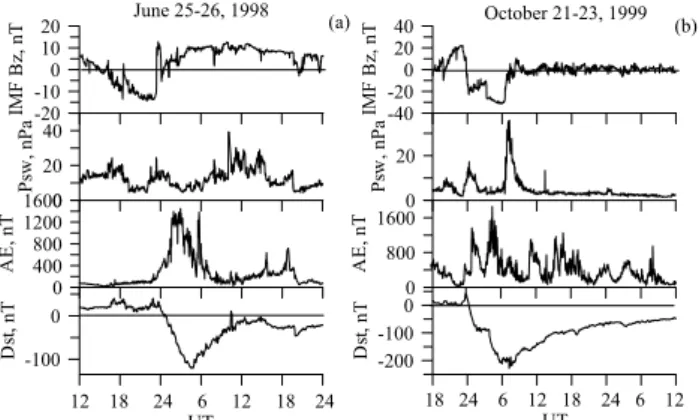
Fig. 1. Overview of 25–26 June 1998 moderate and 21–23 October 1999 intense storm events.
Thus, based only on the measurements, we cannot ex-plicitly distinguish between the contributions from differ-ent magnetospheric currdiffer-ent systems which contribute to the ground magnetic field. However, we can estimate them by using modern magnetospheric models, which can provide separate calculations of the magnetic field of the different magnetospheric magnetic field sources. Magnetic field mod-elling is a useful tool for studying the evolution of large-scale current systems during magnetic storms.
The empirical models developed by Tsyganenko (for ex-ample, T96 (Tsyganenko, 1995) and earlier versions) are constructed by minimizing the RMS deviation from the large magnetospheric database (Fairfield et al., 1994), which con-tains magnetospheric magnetic field measurements accu-mulated over many years. As magnetic storms are rela-tively rare events during the observation period, their in-fluence on the model coefficients is small. The applica-bility of the T96 model is limited to 20>Dst>−100 nT,
0.5 nPa<Psw<10 nPa,−10 nT<BzIMF<10 nT. The version
T01 (Tsyganenko, 2002a,b) was developed using a larger database which also includes measurements made in recent years. It is valid over a wider range of parameter values.
The existing theoretical models determine the magne-tospheric magnetic field from physical constraints. The paraboloid model of the Earth’s magnetosphere (Alexeev, 1978; Alexeev et al., 1996; Alexeev et al., 2001) is based on an analytical solution of the Laplace equations for each large-scale current system in the magnetosphere with a fixed shape (paraboloid of revolution). The paraboloid model takes pa-rameters of magnetospheric current systems (intensities and locations) as input. These input parameters are determined from empirical data using submodels. Such a feature allows for easy changes to the paraboloid model parameterization.
Several types of studies require an accurate representation of the magnetospheric configuration during a specific event. For such cases, event-oriented modelling is of key impor-tance (Ganushkina et al., 2002, 2004). Event-oriented mod-els contain free parameters whose values are evaluated from observations for each time period separately.
The main focus of this paper is the relation between the ring current and the tail current during storm times. To study this we use three different magnetic field models: the paraboloid model (Alexeev, 1978; Alexeev et al., 2001), the event-oriented model (Ganushkina et al., 2002), and the T01 model (Tsyganenko, 2002a,b). To investigate the tail cur-rent/ring current relationship we model two storm events, one moderate storm on 25–26 June 1998, whenDst reached
−120 nT and one intense storm on 21–23 October 1999, in whichDstdropped to−250 nT. Comparison of the magnetic
field given by different models with satellite data allows us to verify the different modelling approaches and their reliability for magnetospheric studies during disturbed conditions. We compute the relative contributions from the ring, magnetotail and magnetopause currents to theDst index using all three
models. Long periods of modelling for each storm allow us to examine and compare the long-term evolution of different current systems during storms with different intensity given by models based on the different approaches.
2 Description of storm events
Figure 1 represents the overview of the measurements during the magnetic storms on 25–26 June 1998 and 21–23 October 1999. The solar wind data and IMF were obtained from Wind spacecraft, taking into account the convection time shift of about 40 min.
On 25 June 1998 the IMFBzbehavior (Fig. 1a) reflected
the passage of a magnetic cloud: southward turn at 15:50 UT whenBzreached−13 nT and then suddenly jumped to more
than +15 nT around 23:00 UT. At 24:00 UT Bz decreased
rapidly to−5 nT and began a new slower enhancement to the level of about 10 nT which is approached at 05:00 UT on 26 June. The solar wind dynamic pressure had several peaks around 20–30 nPa. TheAEindex showed the first increase at about 23:00 UT on 25 June but the maximum substorm ac-tivity was detected during 02:00–04:00 UT on 26 June with a peak value of 14:00 nT around 02:55 UT. TheDst index
started to decrease at the beginning of 26 June and reached −120 nT around 05:00 UT, six hours later the first northward Bz reversal occurred, after a long period of substorm
activ-ity when IMFBzdemonstrated relatively slow growth from
−5 nT to +10 nT. The detailed analysis and interpretation of this interesting phenomena was made by Ohtani et al. (2001). Figure 1b shows an overview of the intense storm on 21– 23 October 1999. IMFBz turned from +20 nT to −20 nT
at about 23:50 UT on 21 October and after some increase during the next three hours dropped down to−30 nT around 06:00 UT on 22 October. After that, the IMFBz oscillated
around zero. Solar wind dynamic pressure showed two main peaks, a 15 nPa peak around 24:00 UT on 21 October and a 35 nPa peak around 07:00 UT on 22 October. There were several peaks in the AE index reaching 800–1600 nT. The Dstindex dropped to−230 nT at 06:00–07:00 UT on 22
3 Storm-time magnetic field models
3.1 Paraboloid model
The basic equations of the paraboloid model represent the magnetic fields of the ring current, of the tail current includ-ing the closure currents on the magnetopause, of the Region 1 field-aligned currents, of the magnetopause currents ing the dipole field and of the magnetopause currents screen-ing the rscreen-ing current (Alexeev, 1978; Alexeev et al., 1996; Alexeev et al., 2001). Here we discuss the latest version of the model, A2000 (Alexeev et al., 2001). In the A2000 model (as in the previous versions of paraboloid model) the magne-topause is set to be a paraboloid of revolution. The condi-tionBn=0 is assumed at the magnetopause. The model
pa-rameters determining the large-scale magnetospheric current systems are the following: the geomagnetic dipole tilt angle ψ, the magnetopause stand-off distanceR1, the distance to
the inner edge of the tail current sheetR2, the magnetic flux
through the tail lobes8∞, the ring current magnetic field
at the Earth’s centerbr, and the maximum intensity of the
field-aligned currentIk. At each moment the parameters of
the magnetospheric current systems define the instantaneous state of the magnetosphere and can be determined from ob-servations.
The A2000 model parameterization is described in detail by Alexeev et al. (2001). The geocentric distance R1 to
the subsolar point is calculated using solar wind data: so-lar wind dynamical pressure and IMFBz component (Shue
et al., 1997). The distance to the inner edge of the tail current sheetR2is obtained by mapping the equatorward boundary
of the auroral oval at midnight,ϕn=74.9◦−8.6 log10(−Dst),
as given by Starkov (1993), to the equatorial plane. The magnetic flux across the tail lobe is a sum of two terms 8∞=80+8s, which depend on the tail current density,R1
andR2. The first term corresponds to a slow adiabatic
evo-lution of the tail current due to solar wind variations and remains constant (80=3.7·108Wb) while the second term
8s=−AL7 π R12
2 q
2R2
R1 +1 is associated with substorms. Here
8s variations represent the integrated substorm activity
de-pendent on the hourly-averaged AL-index (see Alexeev et al., 2001).
According to Burton et al. (1975) and the Dessler-Parker-Sckopke relation (1) the ring current magnetic field variation at the Earth’s center is given bydbr
dt =F (E)− br
τ, whereF (E)
is the injection function defined in accordance with Burton et al. (1975); O’Brien and McPherron, (2000), andτ is the lifetime of the ring current particles. Burton et al. (1975) and O’Brien and McPherron (2000) found the average val-ues of the amplitude of the injection function (d in nota-tion of (Burton et al., 1975; O’Brien and McPherron, 2000)), but apparently it varies from storm to storm. In Alexeev et al. (2001)dwas obtained from independent research by Jor-danova et al. (1999). In these case studies we will find d which provides the minimum RMS deviation betweenDst
and the modelledDst. In such an approachbr will include
not only a contribution from the symmetrical ring current but also the symmetrical magnetic fields from the other magne-tospheric magnetic field sources, which are not included in A2000. First of all, this is the symmetrical part of the partial ring current magnetic field.
Ik is determined from the IMFBz component, and solar
wind velocity and density as described by Alexeev and Feld-stein (2001).
As a result the A2000 allows one to calculate the magnetic field depending on the described above parameters of magne-tospheric current systems, which can be obtained from input data: date, IMF, solar wind density and velocity,ALandDst
indices.
3.2 Event-oriented model by Ganushkina et al.
The Ganushkina et al. (2002, 2004) storm-time magnetic field model (G2003) used the Tsyganenko T89 magnetic field model (Tsyganenko, 1989) as a baseline, and the ring, tail and magnetopause currents were modified to give a good fit with in-situ observations.
The ring current model consists of symmetric and asym-metric parts (Ganushkina et al., 2004) represented by a Gaus-sian distribution of the current density. The total current den-sity of the symmetric ring current is a sum of eastward and westward current intensities. The asymmetric partial ring current is closed by field-aligned currents flowing from the ionosphere at dawn and into the ionosphere at dusk, in the Region 2 current sense. The magnetic field from this current system is calculated using the Biot-Savart law. For the tail current system both global intensification of the tail current sheet and local changes in a thin current sheet were imple-mented (Ganushkina et al., 2004). To adjust for the magne-topause inward motion during increased solar wind dynamic pressure, the magnetic field of the Chapman-Ferraro currents BCFT89 at the magnetopause was scaled using the solar wind
dynamic pressure.
The free parameters in the model are the radial distance of the westward ring current (R0west) and partial ring current
(R0part), and the maximum current densities for westward
(J0west) and partial (J0part) ring currents, the amplification
factor for the tail current (AT S), and the additional thin cur-rent sheet intensity (Antc). By varying the free parameters
we found the set of parameters that gives the best fit between the model and the in-situ magnetic field observations. The details of the fitting procedure can be found in Ganushkina et al. (2002).
3.3 Tsyganenko T01 model
25 20 15 10 5 0 -5 -10 -15 X, Re -15 -10 -5 0 5 10 15 20 25 Y, R e
June 25-26, 1997
GOES 8
GOES 9
Polar Geotail
10 5 0 -5 -10 -15 X, Re -10 0 10 20 30 Y, R e
October 21-23, 1999
GOES 8
GOES 10
Polar Geotail
(a) (b)
15 10 5 0 -5 -10 -15 X, Re -15 -10 -5 0 5 10 15 Z, R e
15 10 5 0 -5 -10 -15 X, Re -12 -8 -4 0 4 8 Z, R e GOES 9 GOES 8 Geotail Polar Polar GOES 8 Geotail GOES 10
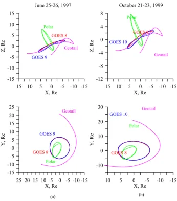
Fig. 2. Evolution of orbits of satellites during the time periods when the magnetic field data was used for modelling storm events on(a) 25–26 June 1997, and(b)21–23 October 1999.
ring current with field-aligned closure currents are included, and the cross-tail current sheet is warped in two dimensions in response to the geodipole tilt, with its inner edge shifting along the Sun-Earth line and its thickness varying along and across the tail. The magnetopause is specified according to the empirical model by Shue et al. (1997).
The model parameters are geodipole tilt angle, IMF By
andBzcomponents, solar wind dynamic pressure, andDst
-index. An attempt is made to take into account the prehistory of the solar wind by introducing two functions,G1andG2,
that depend on the IMFBzand solar wind velocity and their
time history.
4 Comparison of modelling results: magnetic field
To contrast and to examine the reliability of the three mod-els, we present here a comparison of the model results with magnetic measurements from various spacecraft during the June 1998 and October 1999 storms. We calculate the mag-netic field along the spacecraft orbits located in the differ-ent regions of space: geostationary orbit (GOES−8,−9, and −10), near-Earth’s tail (Geotail), and high-latitude magneto-sphere (Polar). Analysis of simultaneous measurements in the different magnetospheric regions helps to determine the role of different magnetospheric current systems during mag-netic storms.
Figure 2 shows the evolution of orbits in the noon-midnight meridional (upper panels) and equatorial (lower
0 5 0 1 0 0
B
x
,
n
T G O E S 8
-1 0 0-5 0 0 5 0 B z, n T 0 5 0 1 0 0
B x , n T -6 0 0 6 0 B z, n T
G O E S 9 Ju n e 2 5 -2 6 , 1 9 9 8
-6 00 6 0 1 2 0
B
x
,
n
T
-1 6 0-8 0 0 8 0 1 6 0
B
z,
n
T
G O E S 8
G O E S 9
P O L A R
P O L A R
-5 5 0 5 5 B x , n T -4 0 0 4 0 B z, n T
1 2 1 8 2 4 6 1 2 1 8 2 4 U T
G E O T A IL
G E O T A IL
0 5 0 1 0 0 1 5 0 2 0 0
B
x
,
n
T G O E S 8
-1 0 0 0
B
z,
n
T
-1 0 00 1 0 0
B
x
,
n
T
-8 00 8 0 1 6 0
B
z,
n
T
G O E S 1 0 O c to b e r 2 1 -2 3 , 1 9 9 9
-1 6 0-8 0 0 8 0 1 6 0
B
x
,
n
T
-1 6 0-8 0 0 8 0 B z, n T
G O E S 8
G O E S 1 0
P O L A R
P O L A R
-5 5 0 5 5 B x , n T -4 0 0 4 0 B z, n T
1 8 2 4 6 1 2 1 8 2 4 6 1 2 1 8 U T
G E O T A IL
G E O T A IL A 20 0 0
(a ) (b )
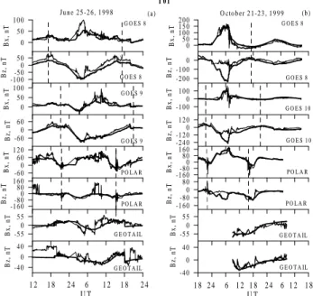
Fig. 3. Comparison of the observedBxandBzcomponents of the
external magnetic field in the GSM coordinates (thin lines) with A2000 model results (thick lines) for GOES 8 (two upper panels), GOES 9 and GOES 10 (next two panels), Polar (next two panels) and Geotail (bottom two panels) for(a)25–26 June 1998 and(b) for 21–23 October 1999 storm events.
panels) planes of satellites such as GOES 8 (red curve), GOES 9 or 10 (blue curve), Polar (green curve), and Geo-tail (pink curve), during the time periods when the magnetic field data were used for modelling storm events on (a) 25–26 June 1997, and (b) 21–23 October 1999. All measurements were made inside the magnetosphere.
Figure 3 shows the Bx and Bz components of the
ex-ternal magnetic field obtained from observations shown by thin lines and A2000 model results shown by thick lines for GOES 8 (two upper panels), GOES 9 and GOES 10 (next two panels), Polar (next two panels) and Geotail (bottom two panels) for (a) 25–26 June 1998 and (b) for 21–23 October 1999 storm events. Dashed grid lines show the noon loca-tions for GOES spacecraft, and perigees of the Polar orbit. Figures 4 and 5 show the observed and model magnetic fields in the same format for the event-oriented model G2003 and the Tsyganenko T01 model, respectively. Bx andBz
mea-sured components represent the main changes in the magne-tospheric current systems. Their comparisons with the model results reveal the main model’s features.
It can be seen that generally all models show quite good agreement with observations. For the moderate storm the Bx measured at geosynchronous orbit is better represented
by the A2000 and T01 models, whereas the G2003 model gives a more accurate reproduction of the Bz component.
The large observedBxvalues imply the existence of intense
Table 1. The RMS deviations in nT between the observed and mod-elled magnetic field calculated by the paraboloid (A2000, Alexeev et al., 2001), event-oriented (G2003, Ganushkina et al., 2003), and Tsyganenko (T01, Tsyganenko, 2002a,b) models during magnetic storms on 25–26 June 1998 and 21–23 October 1999.
Satellites A2000 G2003 T01
25–26 June 1998
GOES 8 18.9 16.8 18.3
GOES 9 21.2 22.4 16.5
Polar 26.7 33.5 28.2
Geotail 28.4 21.0 21.6
21–23 October 1999
GOES 8 37.0 30.2 32.1
GOES 10 33.7 29.4 32.7
Polar 40.0 35.4 32.7
Geotail 22.6 11.8 11.4
the G2003 model. The A2000 model represents the mag-netopause size variations, depending not only on solar wind pressure but also on IMFBz based on Shue et al. (1997)
model. The A2000 describes theBxvalues during the
mag-netic storm main phase (the first 6 h of 26 June 1998) more accurately than the other models. On the other hand, the A2000 model underestimates theBzvalues during this time
interval. This is because the paraboloid model represents the cross-tail currents as a discontinuity between the oppositely directed magnetic field bundles in the southern and northern tail lobes and as a result gives a very smallBzcomponent in
the vicinity of the tail current.
In general, all three models show approximately similar accuracy in the representation of magnetic field data ob-served by Polar. The G2003 model magnetic field agrees with the observed field at Geotail (from 00:20 UT, 25 June until 18:00 UT 26 June while the spacecraft was inside the magnetosphere) slightly better than that given by the A2000 and T01 models.
During the intense storm on 21–23 October 1999 theBx
components from GOES 8 and GOES 10, and Polar, are best represented by the T01 model. At the same time, the T01 model underestimates theBz component significantly at the
storm maximum. ModelBz values were equal to−230 nT
and−250 nT around 06:00 UT on 22 October 1999 while the observed ones were−50 nT and−80 nT at GOES 8 and GOES 10, respectively. At that time, GOES 8 was around midnight and GOES 10 was moving toward midnight in the dusk sector. At the storm maximum, Polar observations on the duskside showedBz=−25 nT while the T01 model gave
Bz=−100 nT. Similarly to the moderate storm, the G2003
model reproduces theBzvariations at GOES and Polar with
enough accuracy.
The local magnetic field variations near the magneto-spheric tail current sheet along the Geotail orbit are not quite correctly reproduced by the models. The A2000 model gives
0 5 0 1 0 0
B
x
,
n
T G O E S 8
-1 0 0-5 0 0 5 0 B z, n T 0 5 0 1 0 0
B x , n T -6 0 0 6 0 B z, n T
G O E S 9 Ju n e 2 5 -2 6 , 1 9 9 8
-6 0 0 6 0 1 2 0
B
x
,
n
T
-1 6 0-8 0 0 8 0 1 6 0
B
z,
n
T
G O E S 8
G O E S 9
P O L A R
P O L A R
-5 5 0 5 5 B x , n T -4 0 0 4 0 B z, n T
1 2 1 8 2 4 6 1 2 1 8 2 4 U T
G E O T A IL
G E O T A IL
0 5 0 1 0 0 1 5 0 2 0 0
B
x
,
n
T G O E S 8
-1 0 0 0
B
z,
n
T
-1 0 0 0 1 0 0
B
x
,
n
T
-8 00 8 0 1 6 0
B
z,
n
T
G O E S 1 0 O c to b e r 2 1 -2 3 , 1 9 9 9
-1 6 0-8 0 0 8 0 1 6 0
B
x
,
n
T
-1 6 0 -8 0 0 8 0 B z, n T
G O E S 8
G O E S 1 0
P O L A R
P O L A R
-5 5 0 5 5 B x , n T -4 0 0 4 0 B z, n T
1 8 2 4 6 1 2 1 8 2 4 6 1 2 1 8 U T
G E O T A IL
G E O T A IL G 2 0 0 3
(a ) (b )
Fig. 4. Observed and model magnetic fields in the same format as in Fig. 3 for the event-oriented model G2003.
0 5 0 1 0 0
B
x
,
n
T G O E S 8
-1 0 0-5 0 0 5 0 B z, n T 0 5 0 1 0 0
B x , n T -6 0 0 6 0 B z, n T
G O E S 9 Ju n e 2 5 -2 6 , 1 9 9 8
-6 0 0 6 0 1 2 0
B
x
,
n
T
-1 6 0-8 0 0 8 0 1 6 0
B
z,
n
T
G O E S 8
G O E S 9
P O L A R
P O L A R
-5 5 0 5 5 B x , n T -4 0 0 4 0 B z, n T
1 2 1 8 2 4 6 1 2 1 8 2 4 U T
G E O T A IL
G E O T A IL
0 5 0 1 0 0 1 5 0 2 0 0
B
x
,
n
T G O E S 8
-2 0 0 -1 0 0 0
B
z,
n
T
-1 0 0 0 1 0 0
B
x
,
n
T
-2 4 0 -1 2 0 0 1 2 0
B
z,
n
T
G O E S 1 0 O cto b er 2 1 -2 3 , 1 9 9 9
-1 6 0-8 0 0 8 0 1 6 0
B
x
,
n
T
-1 6 0 -8 00 8 0
B
z,
n
T
G O E S 8
G O E S 1 0
P O L A R
P O L A R
-5 5 0 5 5 B x , n T -4 0 0 4 0 B z, n T
1 8 2 4 6 1 2 1 8 2 4 6 1 2 1 8 U T
G E O T A IL
G E O T A IL T 0 1
(a )
(a ) (b )
Fig. 5. Observed and model magnetic fields in the same format as in Fig. 3 for the the empirical T01 model.
additional discrepancies (e.g.Bx drops) that arise from the
construction of the tail current model discussed above. How-ever, for both storm events theBxcomponents are described
with a reasonable accuracy at GOES 8 and GOES 10, as well as at Polar.
Table 1 shows the RMS deviations between the satel-lite measurements and model calculations determined as δB=
q 1 N
PN
i=1(Bobs−Bmodel)2. The obtained discrepancies
and include quiet as well as disturbed periods. We note that for each orbit the models give the accuracy of about half of the average value of the magnetic field. In general, all models represent well the global variations of magnetospheric mag-netic field measured by spacecraft. However, the model fea-tures determine the specific behavior of the magnetic field calculated in different magnetospheric regions by different models during the different phases of the considered mag-netic storms.
The paraboloid model reproduces well theBxcomponents
of the magnetic field measured along the GOES and Polar or-bits for any level of disturbances but underestimates theBz
depression, due to tail current model features and possibly due to the absence of the partial ring current model in A2000. The T01 model also provides good agreement between the observed and modelledBx component. On the other hand,
during the intense storm maximum, the modelBzis
signif-icantly more depressed than that observed along the GOES and Polar orbit. Because the ring current cannot give the significant contribution to the magnetic field at geostationary orbit, we propose that this discrepancy is due to an overesti-mation of the tail current contribution. Apparently, this is the consequence of the general approach used in development of any empirical model. Calculation results are very sensitive to the database used for the model construction. Intense storms are only a small part of such databases. As a result just during extremely disturbed conditions the empirical model demon-strates the sufficient discrepancies. The event-oriented model G2003 represents better the substorm-associated variations of theBz component at geosynchronous orbit during both
moderate and intense storms, but gives discrepancies in the Bxvariation during storm maximum.
5 Comparison of modelling results:Dst index
5.1 Model calculations ofDst index
In this study, along with Alexeev et al. (2001), we suggest that the magnetopause, tail and ring currents are the main contributors to theDst index. Although the models
consid-ered above are also able to calculate the magnetic field from the other magnetospheric currents (see Sect. 3), their contri-butions toDst are not addressed in this study.
The storm-time magnetic field depression at the Earth’s surface is determined mainly by ring current, tail current and partial ring current. However, their relative strength and loca-tion in the inner magnetosphere remains ambiguous, and it is difficult to separate in the measurements the partial ring cur-rent from the storm-time tail and symmetrical ring curcur-rents. Obviously, the magnetic field of the partial ring current has a symmetrical part which contributes to theDst-index. The
different estimates for the effect of the partial ring current on Dst were obtained by Liemohn et al. (2001), as the
domi-nant contribution during the magnetic storm main phase, and by Tsyganenko et al. (2003), as about 1/7 of the total ring current contribution during storm maximum. Because the
question about the partial ring current contribution toDst
re-quires special consideration, it will not be the subject of this paper. Along with Ganushkina et al. (2002), we propose in our calculations that the partial ring current produces a part of the total ring current magnetic field variation measured at the Earth’s surface. Actually, it is included in the ring cur-rent magnetic field calculated in terms of the G2003 and T01 models.
Moreover, the partial ring current is not included in the A2000 model. Possibly, this is the reason for the discrep-ancies found during comparison between the model calcula-tions and data measured along the spacecraft orbits. How-ever, the symmetrical part of its magnetic field is included in the ring current magnetic field in terms of the approach used forbr calculation (see Sect. 3.1). So, A2000 allows one
to calculate the total symmetrical ring current magnetic field (originated from both symmetrical and partial ring current) as well as the total ring current contribution toDst
Earlier studies have given different relative contributions from the magnetospheric current systems to theDst index.
These differences can be very large: the tail current contri-bution toDst was∼25% in a study by Turner et al. (2000)
while the tail current contribution was comparable to theDst
in Alexeev et al. (2001) for the same event on 9–12 January 1997. In the present paper we calculate the magnetopause, ring and tail currents storm-time variations at the Earth’s sur-face. The contribution of the ground induced currents to the measured perturbation field is assumed to be 30% of the magnetic perturbation at the Earth’s surface (H¨akkinen et al., 2002). The magnetic field horizontal components (1H (t )) were computed from the external current systems at the lo-cations of six near-equatorial stations (geomagnetic latitude and longitude are in brackets): Sun Juan (29.9◦, 8.2◦), Tener-ife (19.8◦, 61.4◦), Tbilisi (36.8◦, 116.6◦), Lunping (17.6◦, 192.0◦), Kakioka (28.3◦, 210.8◦), Honolulu (21.8◦, 268.7◦) and Del Rio (39.0, 324.1). Then, the quietest day of the month was determined using the World Data Center cat-alogue, and the magnetic field variation during this quiet day, 1Hq(t ), was calculated from the model. The model
Dst(SY M−H )is then
Dst (t )= 1 N
N X
i=1
1Hi(t )−1Hqi(t )
cosθi
, (2)
whereN is the number of stations (6), andθi represents the
magnetic latitudes of the stations. This procedure was re-peated for total Dst and for contributions from the
differ-ent currdiffer-ent systems. This method of Dst computation is
similar to the official procedure described by Sugiura and Kamei (1991). It allows us to unambiguously derive theDst
variations arising from changes in the magnetospheric cur-rent systems in the various models.
5.2 ModelDst index and its sources
June 17, 1998
mp
mp mp
October 20, 1999
tc -20 -10 0 10 20 30 Ds t, n T rc tc
7 8 9 10 11 12 13 14 15 16 UT -8 -4 0 4 8 Ds t, nT -20 -10 0 10 20 Ds t, n T rc tc
7 8 9 10 11 12 13 14 15 16 UT -4 0 4 Ds t, nT -20 -10 0 10 20 30 Ds t, n T rc
0 2 4 6 8 10 12 14 16 18 20 22 24 UT -12-8 -40 4 8 12 Ds t, nT mp -30 -20 -10 0 10 20 Ds t, n T rc tc
7 8 9 10 11 12 13 14 15 16 UT -20 -10 0 10 Ds t, n T G2003 A2000 mp -20 0 20 Ds t, n T rc
0 2 4 6 8 10 12 14 16 18 20 22 24 UT -4 0 4 8 12 Ds t, nT T01 mp -30 -20 -10 0 10 20 Ds t, n T rc
0 2 4 6 8 10 12 14 16 18 20 22 24 UT -20 -10 0 10 Ds t, n T tc tc (a) (b) (c)
Fig. 6.Dst index (black) and the model contributions to the
quiet-time magnetic field at the Earth’s equator from the magnetopause current (green), ring current (red) and tail current (blue) (top panel) together with the total observedDst (black) and modelled quiet-day variation,δHq, (purple) (bottom panel) for 17 June 1998 (left) and 20 October 1999 (right) using(a)A2000 paraboloid model,(b) G2003 event-oriented model, and(c)T01 model, respectively.
October 1999 storms. The average quiet time fields were −0.58 nT and 2.74 nT, respectively.
Figure 6 shows an analysis of the model current contri-butions to the quiet-timeDst-index for 17 June 1998 (left)
and 20 October 1999 (right), using (a) the A2000 paraboloid model, (b) the G2003 event-oriented model, and (c) the T01 model, respectively. The ground-induced currents’ effect (30% of the variation) was taken into account in all the cal-culations.
We can see that the amplitudes of the calculated variations are about 8–10 nT for all the models (see the bottom pan-els), but the average values are different. The average quiet day magnetic field variations computed from the A2000 and G2003 models are close to zero. They are about−5 nT for both events in terms of the A2000 model and about 0 nT and 2.5 nT in terms of the G2003 model. Thus, the magnetic field variation calculated at the Earth’s surface by these models during the disturbed conditions can be taken asDst.
How-ever, the contributions from the individual current systems to Dst are, of course, not zero. Unlike the A2000 and G2003
models, the T01 model gives a quiet day magnetic field
varia-June 25-26, 1998
mp
mp mp
October 21-23, 1999
tc -160 -80 0 80 Ds t, n T rc tc -160 -80 0 Ds t, nT -160 -80 0 80 Ds t, n T rc tc -160 -80 0 Ds t, nT -300 -200 -100 0 100 Ds t, n T rc -300 -200 -100 0 Ds t, nT mp -160 -80 0 80 Ds t, n T rc tc -160 -80 0 Ds t, n T G2003 A2000 mp -300 -200 -100 0 100 Ds t, n T rc -300 -200 -100 0 Ds t, nT T01 mp -300 -200 -100 0 100 Ds t, n T rc -300 -200 -100 0 Ds t, n T tc tc (a) (b) (c)
12 18 24 6 12 18 24 UT
12 18 24 6 12 18 24 UT
12 18 24 6 12 18 24 UT
18 24 6 12 18 24 6 12 18 UT
18 24 6 12 18 24 6 12 18 UT
18 24 6 12 18 24 6 12 18 UT
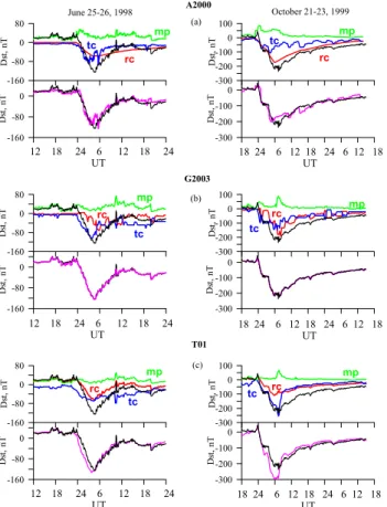
Fig. 7. Model contributions toDstand totalDstduring 25–26 June
1998 and 21–23 October 1999 storm events in the same format as in Fig. 5. The quiet-time contributions from the different current systems are subtracted from the model magnetic field variations.
tion of about−20 nT. Subtracting this value from the ground magnetic field variation during disturbed conditions is an im-portant step in theDst calculations by the T01 model.
It is important to note that the different quiet-time levels are features of the models and possibly are not connected with the real quiet level magnetic field. In particular, it seems that the large quiet-time field in the T01 model is caused by a relatively small number of measurements in the inner mag-netosphere in the database used for T01 construction Tsyga-nenko et al. (2002a,b). The question about the real quiet time magnetic field level at the Earth’s surface remains open for now (see Greenspan and Hamilton (2000).
Figure 7 shows the model contributions and totalDst
dur-ing 25–26 June 1998 and 21–23 October 1999 storm events in the same format as in Fig. 6. The quiet time level and quiet time contributions from the different current systems are sub-tracted from the model magnetic field variations. In general, all three models provideDst, which is in good agreement
with the observedDstindex.
The tail current in the T01 model develops even earlier than theDst starts to decrease. During the storm main phase all
models show that the tail and ring current have comparable contributions to theDst. During the recovery phase the ring
current remains more enhanced than the tail current accord-ing to A2000 and G2003 models, although the G2003 model provides even more tail current contribution than the A2000 model. The ring current in the T01 model recovers rapidly and the tail current remains at an enhanced level almost until the end of the storm recovery.
The situation is quite different during the intense storm on 21–23 October 1999. In all three models the tail current de-velops first whenDst begins to decrease in a manner similar
to the tail current behavior during the moderate storm. Dur-ing the storm maximum the rDur-ing current is the dominant con-tributor to theDstindex in the A2000 and G2003 models. In
the T01 model the tail current continues its development un-til the storm maximum and gives a major contribution to the Dst index, whereas the ring current contributes only about
one third of the tail current contribution. During the recov-ery phase the tail current contribution decreases and becomes comparable to the ring current contribution.
The tail current contribution to theDst index computed
from the A2000 and G2003 models changes during the mag-netic storm. It correlates with substorm activity, and ap-proaches its maximum during substorm maximum estimated by AE enhancement. On the other hand, the ring current cor-relates with the totalDst, and its maximum tends to be near
the Dst maximum. During the moderate storm, the
maxi-mum tail and ring current contributions toDst were about
70% and 50% of maximumDst in the A2000 model, 85%
and 50% of maximumDst in the G2003 model, and 50% and
50% of maximumDst in the T01 model. During the intense
storm the maximum tail and ring current contributions were, respectively, about 50% and 90% for A2000, 70% and 90% for G2003, and 100% and 40% for T01 (note that theDst
sources reach their maximums at different UTs). Ring cur-rent contribution is determined by injection intensity. Am-plitude of the injection function F (E) (see Sect. 3.1) cal-culated in A2000 for the magnetic storm on 21–23 October 1999 d=−3.8nT / h(mV /m)−1 exceeds by absolute value d=−2.8nT / h(mV /m)−1calculated during the 25–26 June 1998 magnetic storm. It looks reasonable to propose that the stronger storm corresponds to the stronger ring current injection and the larger amplitude of injection (by absolute value). However, this conclusion requires more detailed sta-tistical consideration.
In general, all the models confirm the assumption that the tail current magnetic field can be sufficiently large to pro-vide a significant contribution to theDst, variation (Alexeev
et al., 1996). However, the global A2000, G2003 and T01 models demonstrate different tail current development dur-ing magnetic storms. While durdur-ing the moderate storm the tail current and ring current have approximately equal maxi-mum contributions toDst during the strong magnetic storm
the models reveal a different behavior. The tail current be-comes the major contributor toDst in the T01 model, while
the tail current contribution is smaller than that of the ring current in the A2000 and G2003 models.
The totalDstcomputed from the T01 model differs
signif-icantly from the measuredDst during the main phase of the
magnetic storm. Comparison with GOES 8 and GOES 10 data also shows that the model Bz is much smaller than
the observed one during the 21–23 October 1999 magnetic storm maximum. Because the ring current magnetic field at geosynchronous orbit is relatively small, the source of the discrepancies inDstand inBzalong the GOES orbit is
prob-ably caused by the strong intensification of the tail current in the model. The T01 model represents wellDst and
space-craft measurements during moderate magnetic storms, but does not match Dst during intense magnetic storm
maxi-mum. This is a known limitation of the empirical models based on the data of satellite measurements. Possibly, the latest Tsyganenko model (Tsyganenko et al., 2003), which is based on the storm-time data, allows one to obtain the more realistic results during strongly disturbed conditions.
The event-oriented G2003 model, which is also based on empirical data, gives excellent results in reproducingDst, as
it uses measurements obtained during the magnetic storm which is modelled. This highlights the complexity of the magnetospheric response to the solar wind driving, and the consequent need for event-oriented modelling.
6 Discussion
Three magnetospheric models based on very different ap-proaches (theoretical, empirical and event-oriented) were used in our calculations of the magnetic field. The solar wind data and geomagnetic indices are used as input for the-oretical A2000 and empirical T01 models, while the entire existing database of the measurements inside the magneto-sphere is the base of the G03 model. The models have the different parameterizations, but we used a unified procedure ofDst andDst-source calculations in terms of all the
mod-els, corresponding to the official procedure ofDstderivation
from data of ground measurements. This procedure includes subtraction of the quietest day effect and takes into account the magnetic field produced by the Earth’s induced currents. Such an approach enables unambiguous determination and accurate comparison of the Dst contributions produced by
the magnetospheric current systems in terms of the A2000, G2003 and T01 models.
in the A2000, T01 and G2003 models were described in de-tail in Alexeev et al. (1996; 2001); Tsyganenko (2002a,b); Ganushkina et al. (2002; 2004). They satisfactorily reflect the main features of the observed current systems but have slightly different geometry and depend on different parame-ters. For example, the tail current system represented by the models consists of cross-tail currents and closure currents on the magnetopause. The different tail current geometry plays a significant role in the magnetic field calculation near the tail current sheet (see the comparison with Geotail measure-ments, Sect. 4) but hardly influences the magnetic field vari-ations at the Earth’s surface. Otherwise, the tail current in-tensity, as well as the geocentric distance to the tail current inner edge, determine strongly theDst dynamics during the
magnetic storm. During storm maximum the tail current is located close to the Earth and becomes sensitive to the so-lar wind dynamic pressure, IMF, and flux content of the tail. So therefore, we would expect that the parameters of the tail current, and consequently its effect on theDst index are
con-trolled by the factors originated from the solar wind and mag-netosphere. The dependence of the model parameters on the external factors (e.g. measured solar wind data) determines the model parameterization. We can see from our calcula-tions that the differences in the parameterization of the mod-els provide the main differences between theDst calculated
by the A2000, G2003 and T01 models.
In spite of the different model’s parameterizations, the re-sults obtained by all the models show that the tail current plays a significant role in the magnetic storm development. Computations of the tail current contribution to Dst using
the A2000, G2003 and T01 models, show that the tail cur-rent contribution toDst can approach values comparable to
the ring current contribution toDst during storm maximum.
The calculations show that 1) the relationship between tail and ring currents depends on magnetic storm intensity, and 2) this relationship changes during the course of the magnetic storm development.
It was shown that the theoretical A2000 and event-oriented G2003 models give a tail current contribution toDst
compa-rable with the ring current contribution during a moderate storm, but that the ring current becomes the dominant con-tributor during an intense storm (see also Ganushkina et al., 2004). Although we did not analyze the substorm related processes, we can conclude that the level of substorm ac-tivity influences the value of the tail current contribution to Dst. We suggest that the tail current can produce its
maxi-mum contribution toDst for moderate storms while the ring
current remains yet undeveloped. During severe storms, the ring current continues to develop while the tail current has al-ready approached its maximum values. In particular, we can see that the hourly AL index can approach approximately the same maximum values during both moderate and intense storms. The magnetic flux through the polar cap, calculated by the paraboloid model (see Sect. 3.1), as well as the po-lar cap area, depend strongly on the level of substorm ac-tivity and do not demonstrate significant growth during in-tense storms in comparison with moderate ones. On the other
hand, the stronger injection amplitude was calculated during the intense magnetic storm on October 1999.
Detailed investigation of tail and ring current dynamics by the A2000 and G2003 models show that the tail cur-rent (as well as other magnetospheric curcur-rents) contribution toDst varies during a magnetic storm. Both models show
similar behavior of theDst sources: the tail current begins
to develop earlier than the ring current and starts to decay while the ring current continues to develop. The magneto-tail global changes during the magnetic storm are controlled mostly by the solar wind and the IMF, but are accompa-nied by sharp variations associated with substorms. The G2003 model (Ganushkina et al., 2002; 2004) reproduces the tail current development, which correlates well with the substorm-associatedAEindex. Clear correlation of the tail current contribution toDst with substorm activity is also
ap-parent in the results obtained from the A2000 model. Magnetic field sources contributing toDst are controlled
by different factors originating in the solar wind, as well as in the magnetosphere, which change nonsynchronously, with different time scales and, consequently, determine the com-plicated dynamics of theDst. Abrupt changes inDst can be
caused either by magnetopause currents in accordance with the IMF and solar wind dynamic pressure pulses, or by tail current variations during substorms. The tail current disrup-tion following substorm onset often influencesDst recovery
(Iyemori and Rao, 1996; Kalegaev et al., 2001). Along with the results of Ohtani et al. (2001), the substorm related activ-ity during 02:00–04:00 UT on 26 June 1998 resulted inDst
decay by 30 nT after the substorm onset. Both A2000 and G2003 models reveal such aDst drop, while the ring current
continued to develop. The positive jump from the tail current after substorm maximum is calculated to be about−40 nT in the A2000 model and about−50 nT in the G2003 model.
7 Conclusions
This study addresses the relation between the ring current and the tail current during storm times. Three different mag-netic field models, the paraboloid model A2000 by Alex-eev (1978), AlexAlex-eev et al. (2001), the event-oriented model G2003 by Ganushkina et al. (2002, 2004), and the T01 model by Tsyganenko (2002a,b) were used to model two storm events. One storm event was moderate withDst=−120 nT,
and another was an intense storm withDst=−250 nT.
In general, all models showed quite good agreement with in-situ observations. The event-oriented model G2003 repre-sented best the substorm-associated variations of theBz
com-ponent at and near geosynchronous orbit during both moder-ate and intense storms. The T01 model provided good agree-ment between the observed and modelledBxcomponent, but
on the other hand, the modelBz was significantly more
de-pressed than that observed during the intense storm. Simi-larly, the A2000 model reproduces well theBxcomponents
The A2000, G2003 and T01 models showed that during the moderate storm the tail and ring current contributions are comparable. All three models showed that the tail cur-rent develops before the ring curcur-rent whenDst starts to
de-crease. During the recovery phase the ring current stays more enhanced than the tail current, according to the A2000 and G2003 model results. The ring current in the T01 model re-covers quickly and the tail current remains at an enhanced level almost until the end of the storm recovery.
Similar to the moderate storm, during the intense storm, in all three models the tail current developed first whenDst
started to decrease. During the storm maximum the ring cur-rent was the dominant contributor to theDst index in the
A2000 and G2003 models. During the early recovery phase the ring current stayed intensified longer than the tail current, becoming comparable to the tail current intensity during the late recovery. In the T01 model the tail current continued to enhance until storm maximum, and gave the largest contribu-tion to theDst index. During the early recovery phase in the
T01 model the tail current contribution decreased rapidly and became comparable to the ring current. Unlike the moder-ate storm in which the theoretical A2000 and event-oriented G2003 models give a tail current contribution toDst
com-parable with the ring current contribution, during the intense storm the ring current becomes the dominant contributor.
The tail current dynamics in the A2000 and G2003 mod-els is correlated well with substorm activity. The tail current enhancement during substorm precedes theDstrecovery, but
the ring current continues to develop after the substorm max-imum. In agreement with Ohtani et al. (2001), the tail current is responsible for aDst increase of about 30 nT. According
to the A2000 and G2003 models, the tail current preintensi-fication level is about−40 to−50 nT.
Magnetic field modelling is a very useful tool not only for the accurate representation of the magnetic field, but also for studies of the evolution of the large-scale current systems. Global models represent well the main features of the mag-netospheric magnetic field, but give some discrepancies in representing local magnetic field features. For such cases, event-oriented modelling can be used to improve the accu-racy of calculations for specific events.
Acknowledgements. We would like to thank K. Ogilvie and R. Lep-ping for the use of WIND data in this paper, World Data Center C2 for Geomagnetism, Kyoto, for the provisionalAE,KpandDst in-dices data. The data were obtained from the Coordinated Data Anal-ysis Web (CDAWeb). GEOTAIL magnetic field data were provided by T. Nagai through DARTS at the Institute of Space and Astro-nautical Science (ISAS) in Japan. The work of N. Ganushkina was supported by the Academy of Finland. The work of V. Kalegaev was supported by Russian Foundation for Basic Research (Grants 01-07-90117 and 04-05-64396) and INTAS (Grant 03–51–3922).
Topical Editor in chief thanks R. Clauer and another referee for their help in evaluating this paper.
References
Alekseyev, I. I.: Regular magnetic field in the Earth’s magneto-sphere, Geomagnetism and Aeronomy, 18, 447–452, 1978. Alexeev, I. I., Belenkaya, E. S., Kalegaev, V. V., Feldstein, Y. I., and
Grafe, A.: Magnetic storms and magnetotail currents, J. Geo-phys. Res., 101, 7737–7747, 1996.
Alexeev, I. I. and Feldstein, Y. I.: Modelling of geomagnetic field during magnetic storms and comparison with observations, J. At-mos. Sol.-Terr. Phys., 63, 331–340, 2001.
Alexeev I. I., Kalegaev V. V., Belenkaya E. S., Bobrovnikov S. Y., Feldstein Y. I., and Gromova L. I.: Dynamical model of the mag-netosphere: case study for 9–12 January 1997, J. Geophys. Res., 106, 25 638–25 693, 2001.
Arykov, A. A. and Maltsev, Yu. P.: Contribution of various sources to the geomagnetic storm field, Geomagnetism and Aeronomy, 33, 67–74, 1993.
Burton, R. K., McPherron, R. L., and Russell, C. T.: An empirical relationship between interplanetary conditions andDst, J. Geo-phys. Res., 80, 4204–4214, 1975.
Campbell, W. P.: The field levels near midnight at low and equato-rial geomagnetic stations, J. Atmos. and Terr. Phys., 35, 1127– 1146, 1973.
Dessler, A. J. and Parker, E. N.: Hydromagnetic theory of geomag-netic storms, J. Geophys. Res., 64, 2239–2252, 1959.
Dremukhina, L. A., Feldstein, Y. I., Alexeev, I. I., Kalegaev, V. V., and Greenspan, M.: Structure of the magnetospheric magnetic field during magnetic storms, J. Geophys. Res., 104, 28 351– 28 360, 1999.
Fairfield, D. H., Tsyganenko, N. A., Usmanov, A. V., and Malkov, M. V.: A large magnetospheric magnetic field data base, J. Geo-phys., Res., 99, 11 319–11 326, 1994.
Ganushkina, N. Y., Pulkkinen, T. I., Kubyshkina, M. V., Singer, H. J., and Russell, C. T.: Modelling the ring current magnetic field during storms, J. Geophys. Res., 107, 10.1029/2001JA900101, 2002.
Ganushkina, N. Y., Pulkkinen, T. I., Kubyshkina, M. V., Singer, H. J., and Russell, C. T.: Long-term evolution of magnetospheric current systems during storms, Ann. Geophys., 22, 1317–1334, 2004,
SRef-ID: 1432-0576/ag/2004-22-1317.
Greenspan, M. E. and Hamilton, D. C.: A test of the Dessler-Parker-Sckopke relation during magnetic storms, J. Geophys. Res., 105, 5419–5430, 2000.
H¨akkinen, L., Pulkkinen, T. I., Nevanlinna H., Pirjola R. J., and Tanskanen E. I.: Effect of induced currents onDstand on mag-netic variations at midlatitude stations, J. Geophys. Res., 107, 10.1029/2001JA900130, 2002.
Hamilton, D. C., Gloeckler, G., Ipavich, F. M., Studemann, W., Wilken, B., and Kremser, G.: Ring current development during the great geomagnetic storm on February 1986, J. Geophys. Res., 93, 14 343–14 355, 1988.
Iyemory, T. and Rao, D. R. K.: Decay of theDst field of
geo-magnetic disturbance after substorm onset and its implication to storm-substorm relation, Ann. Geophys., 14, 608–618, 1996. Jordanova, V. K., Torbert, R. B., Thorne, R. M., Collin, H. L.,
Roeder, J. L., and Foster, J. C.: Ring current activity during the earlyBz<0 phase of the January 1997 magnetic cloud, J. Geo-phys. Res., 104, 24 895–24 914, 1999.
Geomagnetism and Aeronomie, 38, 10–16, 1998.
Kalegaev V. V., Alexeev, I. I., and Feldstein, Y. I.: The Geotail and Ring Current Dynamics Under Disturbed Conditions, Journal of Atm. and Sol-Terr. Phys., 63, 473–479, 2001.
Kaufmann T. G.: Substorm currents: Growth phase and onset, J. Geophys. Res., 92, 7471–7481 1987.
Liemohn, M. W., Kozyra, J. U., Thomsen, M. F., Roeder, J. L., Lu, G., Borovsky, J. E., and Cayton, T. E.: Dominant role of the asymmetric ring currentin producing the stormtimeDst∗, J. Geophys. Res., 106, 10 883–10 904, 2001.
Maltsev Y. P., Arykov, A. A., Belova, E. G., Gvozdevsky, B. B., and Safargaleev, V. V.: Magnetic flux redistribution in the storm time magnetosphere, J. Geophys. Res., 101, 7697–7704 1996. O’Brien, T. P. and McPherron, R. L.: 2000, An empirical phase
space analysis of ring current dynamics: Solar wind control of injectionand decay, J. Geophys. Res., 105, 7707–7719, 2000. Ohtani, S., Nose, M., Rostoker, G., Singer, H., Lui, A. T. Y., and
Nakamura, M.: Storm-substorm relationship: Contribution of the tail current toDst, J. Geophys. Res., 106, 21 199–21 209, 2001. Sckopke, N.: A general relation between the energy of trapped
par-ticles and the disturbance field near the Earth. J. Geophys. Res., 71, 3125–3130, 1966.
Shue, J.-H., Chao, J. K., Fu, H. C., Russell, C. T., Song, P., Khurana, K. K., and Singer, H. J.: A new functional form to study the solar wind control of the magnetopause size and shape, J. Geophys. Res., 102, 9497–9512, 1997.
Starkov, G. V.: Planetary morphology of the aurora, In
Magnetosphere-Ionosphere Physics, St-Petersburg: Nauka, 85– 90, 1993.
Sugiura, M. and Kamei, T.: EquatorialDst index 1957–1986, in
IAGA Bull. 40, Edited by A. Berthelier, and M. Menvielle, Int Serv. of Geomagn. Indices Publ. Off., Saint Maur, France, 1991. Tsyganenko, N. A.: A magnetospheric magnetic field model with a
warped tail current sheet, Planet. Space Sci., 37, 5–20, 1989. Tsyganenko, N. A.: Modeling the Earth’s magnetospheric magnetic
field confined within a realistic magnetopause, J. Geophys. Res., 100, 5599–5612, 1995.
Tsyganenko, N. A.: A model of the near magnetosphere with a dawn-dusk asymmetry: 1. Mathematical structure, J. Geophys. Res., 107, 10.1029/2001JA0002192001, 2002a.
Tsyganenko, N. A.: A model of the near magnetosphere with a dawn-dusk asymmetry: 2. Parameterization and fitting to obser-vations, J. Geophys. Res., 107, 10.1029/2001JA900120, 2002b. Tsyganenko, N. A., Singer, H. I., and Kasper, J. C.: Storm-time
dis-tortion of the magnetosphere: How severe can it get? J. Geophys. Res., 108, 10.1029/2002JA009808, 2003.