Journal of Computer Science 4 (11): 897-902, 2008 ISSN 1549-3636
© 2008 Science Publications
Corresponding Author: Mwaffaq A. Abu Al hija, Department of Computer Science, Hail University, Hail, Saudi Arabia
A Heapify Based Parallel Sorting Algorithm
1
Mwaffaq A. Abu Al hija,
2Arwa Zabian,
3Sami Qawasmeh and
4Omer H. Abu Al haija
1
Department of Computer Science, Hail University, Hail, Saudi Arabia
2
Department of Computer Science, Jadara University, Irbid, Jordan
3
Department of Computer Science, Irbid National University, Irbid, Jordan
4
Department of Computer Science, Irbid, Jordan
Abstract: Quick sort is a sorting algorithm whose worst case running time is (n2 ) on an input array of n numbers. It is the best practical for sorting because it has the advantage of sorting in place. Problem statement: Behavior of quick sort is complex, we proposed in-place 2m threads parallel heap sort algorithm which had advantage in sorting in place and had better performance than classical sequential quick sort in running time. Approach: The algorithm consisted of several stages, in first stage; it splits input data into two partitions, next stages it did the same partitioning for prior stage which had been spitted until 2 m partitions was reached equal to the number of available processors, finally it used heap sort to sort respectively ordered of non internally sorted partitions in parallel. Results: Results showed the speed of algorithm about double speed of classical Quick sort for a large input size. The number of comparisons needed was reduced significantly. Conclusion: In this study we had been proposed a sorting algorithm that uses less number of comparisons with respect to original quick sort that in turn requires less running time to sort the same input data.
Key words: Parallel sorting, heap sort, Quick sort, in-place sorting
INTRODUCTION
Sorting is one of the most well studied problems in computer science because it is fundamental in many applications. Quick sort [1] is typically the fastest sorting algorithm, basically due to better cache behavior among other factors. However, the worst case running time for Quick sort is O (n2) for an input size n, which is unacceptable for large data sets. In this study, we propose PSA Partition and Swap Algorithm, which reduces the time needed for sorting with respect to Quiksort in the worst case. A comparison between Quick sort and PSA algorithm in terms of running time is performed; the simulation results show that PSA is faster than Quick sort in the worst case for sorting the same input data size. Our algorithm is based on partitioning the input data to different partitions then using Heapify procedure in parallel to sort each partition. The heap is a very fundamental data structure used in many application programs. A heap is a data structure that stores an array in a binary tree maintaining two properties: the first is that the value stored in every node is smaller than or equal to the value of its children. The second property is that the binary tree must be complete. This implies that the
complete binary tree with height h has between 2h and 2h+1 -1 node. So, the height of a binary tree of n nodes is O (log2 n). The basic operations of the heap are
Build-Heap and Build-Heapify. Build-Heapify operation arranges the heap to restore its heap property.
MATERIALS AND METHODS
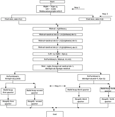
Partition and Swap Algorithm (PSA): Given an array of size n, PSA divides the array into four sub-arrays in two steps to facilitate the sorting and to reduce the number of comparisons needed. The algorithm works in three phases the first partition phase, the second partition phase and finally the Heapify phase.
In the first partition phase the algorithm divides the array A[n] into two sub-arrays A1, A2 based on the
middle value midval, in a manner that all the elements of A1 (or denoted left) are smaller than the midval and
all the elements of A2 (or denoted as right) are greater
than the (midval), if the data must be ordered in an ascendant manner. (If the data must be ordered in descendent manner, all the elements of A1 must be
greater than the midval and all the elements of A2 must
A1l, A1r and A2 is divided into two sub arrays A2l, A2r
then the elements of these four sub arrays are ordered as in the previous phase. The third phase, is heavily phase in which the resultant subarrays A1l, A1r, A2l, A2r are
organized using heavily procedure into sorted subarrays.
First partition phase:
• Given an array A of size n find the middle location of the n elements the pivot can be find by n/2 . Step 1 in the flowchart
• For each part (left and right to the pivot) find the max and min values (step 2 in the flowchart) • Find the mid value midval that can be calculated as
following:
Lmax + Lmin+ Rmax+Rmin /4
• For each element in the two subarrays A1 (left), A2 (right) do the following comparisons (if the array is ordered in an ascendant manner) For i, j are two pointers,
A[0], A[n] denote the first and last element in the array
Swap procedure:
for i = 0 to n/2, j = n to n/2 do:
if A[0] = Lmax > midval and
Rmin = A[n]< Lmax
Swap (Rmin, Lmax )
if i ≠ j
i = i+1, j = j+1 Return if Else End Else
i = i+1 and Return if
The procedure stops when i = j, that means the two pointers are encountered and all the elements on the left and on the right have been visited and compared. This condition is important to ensure the correctness of the algorithm and to ensure that all the elements have been compared. In the case of n being an odd number, we take n/2 to find the mid location (pivot location),
Fig. 2: PSA algorithm/first partition phase
in which case the right will have more elements than the left and the pointer i must continue to visit the elements until it encounters j.
Second partition phase: The algorithm starts working in parallel in dividing the two subarrays A1, A2 to four
consecutive partitions A1l, A1r, A2l, A2r and the swap
procedure will be repeated for the following counters in A1 for i = 0 to n/4, j = n/2 to n/4 and for A2 the counter
will be: for i = n/2 to 3n/2, j = n to j = 3n/2.
At the end of this phase we obtain four subarrays in such a manner that:
All the elements of A1l < all the elements of A1r and all
the elements of A2l < all the elements of A2r
Heapify phase: In this phase, we use heavily procedure on all the four resultant sub-arrays to organize them in sorted subarrays.
Figure 1 shows the flowchart that describes how PSA work. In the first step of the flowchart the initial array is divided into two sub-arrays and the midval-location is found. In the second step, the min and max values for each partition are found and a series of swap operations are done. Step 3 indicates the last phase that is heavily phase.
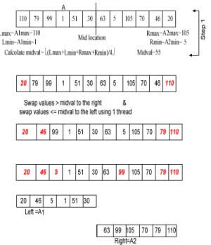
Example: Figure 2 shows a numerical example of how PSA works in an array of size n = 12. In Fig. 2, A is divided into two sub-arrays A1, A2 where the bold items
Fig. 3: PSA algorithm/merge in place
Fig. 4: PSA Algorithm/ Heapify Phase
represent the swapped elements. In part A of Fig. 3, the sub-array A1 is divided, to left1 and right1. In part B,
A2 is divided into two sub-arrays left 2, right 2. In
Fig. 4, it is shown how the four sorted sub-arrays are inserted in their location into the final sorted array.
RESULTS
Input size
R
u
n
n
in
g
t
im
e
(m
s)
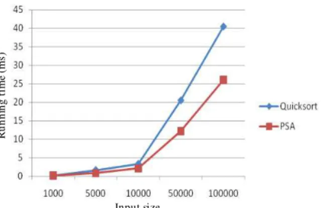
Fig. 5: The running time of both Quick sort and PSA algorithms
Input size
#
o
f
c
o
m
p
ar
is
o
n
s
Quicksort
Fig. 6: The number of comparisons needed to sort the same input size in both Quick sort and PSA algorithms
For an input size 1000-5000 the performance of PSA is similar to that of Quick sort.
However, for a large data size (100.000) PSA outperforms Quick sort (Fig. 5). Figure 6, shows that there a big difference in the number of comparisons needed to sort the same input data between both Quick sort and PSA, where PSA requires a less number of comparisons with respect to Quick sort in all the input data sizes tested.
DISCUSSION
Our goal in this study is to propose an algorithm that performs better than Quick sort in term of running time. However the performance of quicksort is optimal only for a large input size. Analyzing the results presented in Table 1 we can see that the efficiency of our algorithm is about 73% for a small input size
Table 1: Comparison between the running time of Quick sort and PSA for different input size
Quick sort running PSA running
Input size time (ms) time (ms)
1000 0.234 0.171
5000 1.640 0.829
10000 3.313 2.139
50000 20.485 12.203
100000 40.460 26.090
(1000 items), however the efficiency of our algorithm respectively to Quick sort is about 64.56% for a large input size and does not change if the input size increased from n to 10 n (10000-100000 items). And that is accorded with our goal is to propose an algorithm simple that works in parallel and has a good efficiency for all input size.
CONCLUSION
In this study we have been proposed a sorting algorithm that uses less number of comparisons with respect to original Quick sort that in turn requires less running time to sort the same input data. Our algorithm is based on dividing the initial array in four partitions in a manner that during the partitioning process the sub-arrays are organized from the smaller to the bigger elements reducing in that the number of comparisons for the final merging operation. In addition it is used the heavily procedure that organize the nodes of each partition in a data structure useful for the searching operation. Our results show that PSA algorithm performs better than original Quick sort for the input data size tested.
Sorting algorithms can be classified into three categories: the first category is based on the number of comparisons in the worst and average and best case. The second category is based on the memory usage and the last category is based on the difference in behavior in the worst case and the average case.
In[2], a comparison between three sorting algorithms (Heap sort[4], Quick sort[3] and Merge sort[5]) is done and a new algorithm is proposed that is a variant of heap sort (modified heap sort). The new algorithm requires nlogn-0.788928 comparisons in the average case. The algorithm uses only one comparison at each node. With one comparison, the algorithm can decide which child of a node contains a larger element and this child is promoted to its parent position.
than the other algorithms. However, for an input size from 5000-50000 quicksort outperforms the other algorithms in terms of execution time. However, for input size 100000 the modified heap sort requires a less running time to sort this input data. In[6], a heap traversal algorithm is proposed that visits the node of a heap and stores its value in an auxiliary data structure with size n/2 , in a manner that the time for locating the next node for traversal is O (log n) in the worst case. The main advantage of the algorithm is that the data structure used is small, which consequently helps in the searching operation. The algorithm takes a min-heap as input and visits the min-heap in ascending order of the value stored in the nodes without making any changes to the structure or contents of the heap. The nodes that are being traversed are copied into another list, producing an ordered list of the values stored in the original heap. The algorithm is similar to an in-order traversal of a binary search tree. A comparison between the running time of generic Quicksort, optimized quicksort (optquicksort), heap sort, heap traversal of a binary tree (heapbt) and the proposed algorithm heap traversal using binary heap (heapbh) is done. The comparison results show that for an input size of 30000 the heapbh performs slightly better than heap sort. An another sorting algorithm that reduces the cache size is proposed in[7], the proposed dualheap sort algorithm partitions recursively the subheaps in half until the subheaps become small to partition any more, then the array is sorted. The algorithm has different advantages in term of more operations and cache size. In the best case where the input is already sorted the dualheap sort performs no move operations and nlogn comparisons. In addition, the continued partitioning of the subheaps decreases the cache size needed in each step. The algorithm constructs two opposing subheap and then exchanges values between them until the larger values are in one subheap and the smaller values are in the other. The results presented in[7] show that dualheap sort performs about (50%) more comparisons and move operations than heap sort but the memory size needed is smaller. In[8], a variant of heap sort is proposed that uses a new data structure for pairs of nodes of which can be simultaneously stored and processed in a single register. The algorithm sorts pair of elements in ascending order. By n/2 comparisons, all larger elements of each pair 2i, 2i+1 can be brought to even positions. To construct the new data structure of size n/2 elements it needs (1+ /2) n comparisons where >0, in contrast to weak heaps[9], that takes n-1 comparisons. In this data structure, during swapping it must swap nodes containing pair of elements with similar nodes at no extra cost. After constructing the heap, in the sorting phase the active elements (the even elements are called active and the other ones dormant)
in the root will be placed in the last unsorted position and perform heavily or heap adjustment. This is to find out the larger or smaller key between the 2nd key of the 1st pair and the 1st key of the last pair. In the new data structure each key require three movements. The experimental results indicate that the new data structure for heaps results in better performance of heap sort algorithm in term of number of comparisons. In[10], is proposed ultimate heap sort that is a variant of heap sort that sorts n elements in (nlog2 (n+1)) time in the worst
case by performing at most nlog2n+θ(n) key
comparisons and nlog2n+θ(n) element moves. The
algorithm transforms the heap on which it operates into two-layer heap which keeps small elements at the leaves. The two layer heap works as follow: first it finds 2d the largest key of the elements in the array where denoted as x. x is the largest power of 2 smaller than or equal to n. Then, it partitions the array A[1..n] into three pieces: A[1…r], A[r+1…….r+e] and A[r+e+1,…….n], in a manner that the key of every element in the three partitions is larger than, equal to and smaller (respectively) to x. Then the array A[1….r] is arranged into a heap using standard heap construction algorithm. In ultimate heap sort, the input array to be sorted of size n is sorted in d-1 rounds. Where d = log2
(n+1) . In each round one half of the elements are sorted. In the first phase of the ith round, I = {1….d-1} the remaining ni elements are built into a two layer
heap. In the second phase of the ith round, the ri elements with a key larger than x are removed from the heap. The removed elements are exchanged with the last ri elements of the heap. In the third phase of the ith round, ni-2di-ri of the elements with a key equal to that
of x are gathered together and moved at the end of the sub-array containing the remaining elements. The computations carried out in each round are the following:
• Rearrange A[1..n] into a two layer heap
• For n steps-1 →j until n-l do: exchange A[1] and A[j], remake A[1………j-1] into heap
REFERENCES
1. Cormen, T., C.E. Leiserson, R.L. Rivest and C. Stein, 2001. Introduction to Algorithms. 2nd Edn., MIT Press and McGraw-Hill. ISBN 10: 0-262-03293-7.
2. Sharma, V., S. Singh and K.S. Kahlon, 2008. Performance study of improved HeapSort algorithm and other sorting algorithms on different platforms. Int. J. Comput. Sci. Network Secur.,
8: 101-105.
3. Hoare, C.A.R., 1962. Quick sort. Comput. J., 5: 10-15. DOI: 10.1093/comjnl/5.1.10.
4. Wegener, I., 1990. Bottom-up heap sort a new variant of heap sort beating on average quicksort. Proceeding of the Mathematical Foundations of Computer Science, Aug. 27-31, Springer-Verlag Inc., Banska´ Bystrica, Czechoslovakia, New York
USA., pp: 516-522.
http://portal.acm.org/citation.cfm?id=90256. 5. Knuth, D.E., 1998. The Art of Programming
Sorting and Searching. 2ndEdn., Addison-Wesley Professional, pp: 780. ISBN: 0-201-89685-0. 6. Mao, L.J. and S.D. Lang, 2003. An empirical study
of heap traversal and its applications. Proceedings of the 7th World Multi Conference on Systematic, Cybernatics and Informatics, July 27-30, Orlando-
Florida, USA., pp: 167-171.
http://www.cs.ucf.edu/csdept/faculty/lang/pub.html. 7. Sepesi, G., 2007. DualHeap sort algorithm: An
inherently parallel generalization of heapsort. http://adsabs.harvard.edu/abs/2007arXiv0706.2893S
8. Shahjala and M. Kaykobad, 2007. A new data structure or heap sort with improved numbers of comparisons. Proceedings of the 1st Workshop on Algorithms and Computation, Feb. 12-12, Dhaka,
Bangladesh, pp: 88-96.
http://teacher.buet.ac.bd/saidurrahman/walcom200 7/proceedings/shahjalal.pdf.
9. Duton, R.D., 1993. The weak heapsort. BIT Numer. Math. J. Part I Comput. Sci., 33: 372-381. http://www.springerlink.com/content/x442k4973j5 242p0/.
10. Katajainen, J., 1998. The ultimate heapsort. Proceedings of the Computing: The 4th Australian Theory Symposium Australian Computer Science Communications, Springer-Verlag. Singapore, pp: 87-95.