Bivariate return period based on copulas for hydrologic dam design: comparison of theoretical and empirical approach

(1)

HESSD

10, 557–596, 2013

Comparison of theoretical and empirical approach

A. I. Requena et al.

Title Page

Abstract Introduction

Conclusions References

Tables Figures

◭ ◮

Back Close

Full Screen / Esc

Printer-friendly Version Interactive Discussion

Discussion

P

a

per

|

Dis

cussion

P

a

per

|

Discussion

P

a

per

|

Discussio

n

P

a

per

|

Hydrol. Earth Syst. Sci. Discuss., 10, 557–596, 2013 www.hydrol-earth-syst-sci-discuss.net/10/557/2013/ doi:10.5194/hessd-10-557-2013

Hydrology and Earth System Sciences Discussions

This discussion paper is/has been under review for the journal Hydrology and Earth System Sciences (HESS). Please refer to the corresponding final paper in HESS if available.

Bivariate return period based on copulas

for hydrologic dam design: comparison of

theoretical and empirical approach

A. I. Requena, L. Mediero, and L. Garrote

Department of Hydraulic and Energy Engineering, Technical University of Madrid, Madrid, Spain

Received: 20 December 2012 – Accepted: 25 December 2012 – Published: 15 January 2013

Correspondence to: A. I. Requena (ana.requena@caminos.upm.es)

(2)

HESSD

10, 557–596, 2013

Title Page

Tables Figures

◭ ◮

Back Close

Full Screen / Esc

Discussion

P

a

per

|

Dis

cussion

P

a

per

|

Discussion

P

a

per

|

Discussio

n

P

a

per

|

Abstract

Hydrologic frequency analyses are usually focused on flood peaks. Multivariate analy-ses on flood variables have not been so exhaustively studied despite the fact that they are required to represent the full hydrograph, which is essential for designing some structures like dams. In this work, a bivariate copula model was used to obtain the

5

bivariate joint distribution of flood peak and volume. An empirical bivariate return pe-riod was defined in terms of acceptable risk to the dam through the maximum water elevation reached during the routing process, in order to perform a risk assessment of dam overtopping. A Monte Carlo procedure was developed to compare the probability of occurrence of a flood with the return period linked to the risk of dam overtopping.

10

The procedure is applied to the case study of the Santillana reservoir in Spain. A set of synthetic peak-volume pairs was generated by the fitted copula and synthetic hy-drographs were routed through the reservoir. Diff_{erent reservoir volumes and spillway}

lengths were considered. Hydrographs with the same risk were represented by a curve in the peak-volume space. These curves were compared to those linked to the

prob-15

ability of occurrence of a flood event, in order to improve the estimation of the Design Flood Hydrograph.

1 Introduction

Univariate flood frequency analyses have been carried out widely, focusing on the study of flood peaks. However, when a hydrological event is characterised by a set of

corre-20

lated random variables, the univariate frequency analyses do not procure a full evalu-ation of the probability of occurrence of the hydrological event (Chebana and Ouarda, 2011). Moreover, the risk related to a specific event can be over or underestimated if only the univariate return period is analysed (De Michele et al., 2005; Salvadori and De Michele, 2004). Therefore, due to the multivariate nature of flood events, a multivariate

(3)

HESSD

10, 557–596, 2013

Title Page

Tables Figures

◭ ◮

Back Close

Full Screen / Esc

Discussion

P

a

per

|

Dis

cussion

P

a

per

|

Discussion

P

a

per

|

Discussio

n

P

a

per

|

frequency analysis of random variables such as flood peak, volume and duration is required to design some structures like dams.

Traditional multivariate techniques assume that the marginal distributions should come from the same family of distributions and the dependence between variables follows a linear relationship. However, drawbacks arise because these assumptions

5

could not be satisfied by the dependence structure of flood variables. Copula models can avoid these diffi_{culties. A copula is a function that connects a multivariate}

dis-tribution function with its univariate marginal disdis-tribution functions using dependence measures among correlated random variables (Nelsen, 1999). The main advantage of copulas is that univariate marginal distributions can be defined independently of the

10

joint behaviour of the variables involved. Hence, a copula allows to model the depen-dence structure of random variables regardless the family that the marginal distribu-tions belong to. Besides, joint return periods can be easily estimated from copulas, which represents an additional benefit as the study of joint return periods is essential to flood frequency analysis.

15

The theory of copulas is based on the Sklar’s theorem (Sklar, 1959), which in the case of a bivariate case can be written in the form:

H(x,y)=_C_{_F₍_x_),_G₍_y₎_}_,_x_,_y _{∈ ℜ} ₍₁₎

whereH(x,y) is the joint cumulative distribution function of the random variablesX and

Y,F(x) andG(y) are the marginal distribution functions ofX andY, respectively, and

20

the mapping functionC: [0, 1]2→[0, 1] is the copula function.

Further details about copulas can be found in Joe (1997), Nelsen (1999) and Sal-vadori et al. (2007).

Although copula models have been extensively applied in other fields such as fi-nance, they have been only recently applied to model hydrological events such as

25

(4)

HESSD

10, 557–596, 2013

Title Page

Tables Figures

◭ ◮

Back Close

Full Screen / Esc

Discussion

P

a

per

|

Dis

cussion

P

a

per

|

Discussion

P

a

per

|

Discussio

n

P

a

per

|

of dependence can be considered. Some authors used Archimedean copulas such as the Frank copula (Favre et al., 2004) or the Clayton copula (Shiau et al., 2006) to char-acterise the dependence structure between peak and volume variables. Meanwhile, extreme value copulas have the advantage that they are able to connect the extreme values of the studied variables, which is very important in flood frequency analysis. A

5

lot of authors considered the Gumbel copula as the copula that best represents the relation between peak and volume (Zhang and Singh, 2006, among others).

But selection of the copula model that best fits the observed data is not a trivial is-sue. Some works have been carried out in recent years regarding the steps required to select a copula model. Using a small sample, Genest and Favre (2007) described

10

diff_{erent aspects to take into account in the process of studying the dependence}

be-tween two random variables, in order to identify the appropriate copula model. The importance of considering upper tail dependence in copula selection was emphasised by Poulin et al. (2007), in order not to underestimate the flood risk, as the upper tail dependence is related to the degree of dependence between the extreme values of the

15

variables involved in the study. Thereby, Chowdhary et al. (2011) indicated the steps needed to select the best copula model taking into account the tail dependence in the decision process.

Moreover, bivariate flood frequency analyses require the estimation of bivariate re-turn periods. Salvadori and De Michele (2004) studied the unconditional and

condi-20

tional return periods of hydrological events using copulas, focussing on the joint return period in which either x or y are exceeded (primary return period) and on the joint return period in which bothx and y are exceeded. An additional return period linked to the primary return period was also introduced, the secondary return period, which is associated with the realization of dangerous events for the dam. Authors such as

25

(5)

HESSD

10, 557–596, 2013

Title Page

Tables Figures

◭ ◮

Back Close

Full Screen / Esc

Discussion

P

a

per

|

Dis

cussion

P

a

per

|

Discussion

P

a

per

|

Discussio

n

P

a

per

|

the generated hydrographs was below the crest level. Klein et al. (2010) presented a methodology to classify floods regarding the hydrological risk, estimating the probabil-ity of occurrence of peak and volume via a copula model. According to the maximum water level reached at the dam, floods were classified in diff_{erent areas from the risk}

associated with the primary return period. Other studies have been carried out

regard-5

ing multivariate flood frequency analysis using copulas (Grimaldi and Serinaldi, 2006; Serinaldi and Grimaldi, 2007; Zhang and Singh, 2007).

In this paper, a bivariate copula model is used for generating a set of synthetic peak-volume pairs. Synthetic hydrographs are estimated using observed hydrographs to be ascribed an adequate shape. Flood hydrographs are routed through a reservoir to

ob-10

tain the maximum water level reached at the dam during the routing process, in order to analyse the hydrological risk of dam overtopping. Both curves that represent the risk to the dam and joint return period curves that represent the probability of occurrence of floods are compared. A sensitivity analysis is carried out on the risk to the dam taking into consideration diff_{erent reservoir volumes and spillway lengths. The methodology}

15

is applied to the Santillana reservoir in Spain.

The structure of the paper is the following: the proposed methodology is shown in Sect. 2. Section 3 presents the case study. Then, the results obtained after applying the procedure are included in Sect. 4. Conclusions are introduced in Sect. 5.

2 Methodology

20

(6)

HESSD

10, 557–596, 2013

Title Page

Tables Figures

◭ ◮

Back Close

Full Screen / Esc

Discussion

P

a

per

|

Dis

cussion

P

a

per

|

Discussion

P

a

per

|

Discussio

n

P

a

per

|

2.1 Copula selection

Identification of the copula that best fits the observations is required, as several fam-ilies of copulas exist. The copula that best represents the dependence structure be-tween variables will be the most appropriate. The steps involved in selecting the appropriate copula model are: (i) dependence evaluation; (ii) parameter estimation

5

method; (iii) goodness-of-fit tests and (iv) tail dependence assessment.

2.1.1 Dependence evaluation

A dependence analysis among correlated random variables is conducted to determine if some kind of dependence really exits. It can be carried out by graphical analyses or dependence measures. A graphical analysis of dependence can be displayed by the

10

scatter plot of the pairs of ranks (Ri,Si) derived from de observed data pairs (Xi,Yi)

(whereR_i is the rank of X_i among X_i, ...,X_n and S_i is the rank of Y_i among Y_i, ...,Y_n, beingi=_{1, ...,}_n_{), the Chi-plot (Fisher and Switzer, 1985, 2001) and the K-plot (Genest}

and Boies, 2003). Besides, dependence measures are needed to procure a quantita-tive value of the dependence relation between variables. For this purpose, the

Spear-15

man’s rho and Kendall’s tau rank based non-parametric measures of dependence are adopted and its associated p-values are estimated (independence between variables is rejected when the p-value is less than 0.05). The result of this evaluation provides an idea of the type of copula to be considered in the study, since each copula supports a particular range of dependence parameter. Michiels and Schepper (2008) provides

20

ranges of admissible Kendall’s tau to diff_{erent copulas for the bivariate case. Therefore,}

the number of feasible copulas can be reduced using the Kendall’s tau value.

2.1.2 Parameter estimation method

The estimation of the copula parameterθ can be performed through diff_erent

meth-ods. A first group consists of rank based methods, in which the parameter estimation is

(7)

HESSD

10, 557–596, 2013

Title Page

Tables Figures

◭ ◮

Back Close

Full Screen / Esc

Discussion

P

a

per

|

Dis

cussion

P

a

per

|

Discussion

P

a

per

|

Discussio

n

P

a

per

|

independent of the marginal functions, such as the method based on the inversion of a non-parametric dependence measure (e.g. the inversion of Kendall’s tau dependence measure) and the maximum pseudo-likelihood method (MPL). Other methods certainly depend on the marginal distributions, such as the inference function for margins (IFM) method proposed by Joe and Xu (1996). There is no consensus, but a large number of

5

authors defend the use of the rank based estimation methods. Supporting this position, Kim et al. (2007) argue that IFM methods are non-robust against misspecification of the marginal distributions, as the parameter estimation depends on the choice of the uni-variate marginal distributions and can be aff_{ected if such models do not fit adequately.}

Consequently, in the present work two rank based methods were used: the inversion

10

of Kendall’s tau method and the maximum pseudo-likelihood method (MPL).

2.1.3 Goodness-of-fit tests

The aim of a goodness-of-fit test is selecting the copula that best represents the de-pendence structure of variables from observed data. Graphical tools and formal tests are provided to achieve this purpose.

15

A first idea of the behaviour of the copulas can be drawn via a scatter plot of the pairs (Ri/(n+1), Si/(n+1)), being nthe observed record length, and a synthetic sample

of pairs generated from each copula of study (U1j,U2j), being j=1, ...,m and m the

sample size. A more useful graph can be elaborated fitting the marginal distributions of the random variables in order to transform the pairs generated from the copula into

20

their original units (X_j,Y_j), following Eq. (2):

(Xj,Yj)=( ˆF−1(U1j), ˆG−1(U2j)) (2)

where ˆF−1and ˆG−1are the quasi-inverses of the marginal distributions functionsF and

G, respectively.

A third graph is the generalized K-plot, based on the procedure introduces by

Gen-25

(8)

HESSD

10, 557–596, 2013

Title Page Abstract Introduction Conclusions References Tables Figures ◭ ◮ ◭ ◮ Back Close

Full Screen / Esc

Printer-friendly Version Interactive Discussion Discussion P a per | Dis cussion P a per | Discussion P a per | Discussio n P a per |

equal or smaller than t. This widely used procedure has been specially designed for Archimedean copulas, so there are circumstances in which a goodness-of-fit test based on it is not consistent. This is the case of extreme value copulas, asK(t) is the same for all of extreme value models (Genest et al., 2006).

Although graphical tools provide a general notion of the goodness-of-fit, formal tests

5

are needed to quantified it. Several procedures have been proposed in the last years. Genest et al. (2009) show a review and analyse various rank-based procedures. These procedures are classified in three groups: tests based on the empirical copula, tests based on Kendall’s transform and tests based on Rosenblatt’s transformation. The re-sults indicate that overall, the Cram ´er-von Mises statistic (S_n) based on the empirical

10

copula has the best behaviour for all copula models, allowing to diff_{erentiate among}

extreme value copulas. It also emphasised the importance of calculating the p-value associated to the goodness-of-fit test to formally prove whether the selected model is suitable. The p-value is obtained through a parametric bootstrap based procedure that was validated (Genest and R ´emillard, 2008). TheSn statistic can be written as:

15

Sn= n

X

i=1

Cn

_R

i

n+₁, S_i n+₁

−Cθn

_R

i

n+₁, S_i n+₁

2

. (3)

where,

C_n(u,v)=1 n

n

X

i=1

1

_R

i

n+₁ ≤u, Si

n+₁ ≤v

,u,vǫ[0, 1]. (4)

beingC_nthe empirical copula (a non-parametric rank based estimator of the unknown copula) andCθn the estimated copula.

20

The Sn statistic based on the empirical copula was the goodness-of-fit test utilised

(9)

HESSD

10, 557–596, 2013

Title Page Abstract Introduction Conclusions References Tables Figures ◭ ◮ ◭ ◮ Back Close

Full Screen / Esc

Printer-friendly Version Interactive Discussion Discussion P a per | Dis cussion P a per | Discussion P a per | Discussio n P a per |

2.1.4 Tail dependence assessment

The idea of tail dependence is connected with the degree of dependence in the upper-right-quadrant tail or lower-left-quadrant tail of a bivariate distribution. More attention is paid on the upper tail dependence, due to the focus of this work on the frequency anal-ysis of extreme flood events. Upper tail dependence is associated with the capacity to

5

link extreme flood peaks to extreme volumes, quantified by the upper tail dependence coeffi_cient _λ_U_{). Which can be interpreted as the conditional probability of} _F₍_x₎_{> w}

givenG(y)> w, when the thresholdwtends to one (Eq. 5).

λU= lim

w→1−P F(x)> w|G(y)> w

. (5)

The copula representation of this coeffi_{cient can be expressed as:}

10

λC_U= _lim

w→1−

1−2w+_C₍_w_,_w₎

1−w . (6)

The graphical analysis of the tail dependence is based on the Chi-plot (Abberger, 2005). A non-parametric estimator of the upper tail dependence coeffi_{cient is obtained}

in order to be compared with the upper tail dependence coeffi_{cient of each selected}

copula. In the present study the considered estimator is ˆλCFG_U (Eq. 7). The estimator

15

was proposed by Frahm et al. (2005). Among others, the estimator has been applied by Serinaldi (2008).

ˆ

λCFG_U =₂₋_{2 exp}    1 n n X

i=1

log      q log_u1

i log

1

vi

log_max(1_u i,vi)2

      

. (7)

The estimator is based on the assumption that the empirical copula can be approx-imated by an extreme value copula. It also works well when this hypothesis is not

20

(10)

HESSD

10, 557–596, 2013

Title Page

Tables Figures

◭ ◮

Back Close

Full Screen / Esc

Discussion

P

a

per

|

Dis

cussion

P

a

per

|

Discussion

P

a

per

|

Discussio

n

P

a

per

|

analysis, copulas that reproduce properly the dependence in the extremes are identi-fied. Because of a good upper tail dependence fit does not mean a good whole data fit, the assessment of the tail dependence is developed at this point and not before. Therefore, the best copula is the copula which represents properly the dependence structure of the variables peak and volume and allows to study adequately the extreme

5

events.

2.2 Joint return periods

The estimation of joint return periods is required in a bivariate flood frequency analysis. The joint return periodT_X∨_,_Y (in which the thresholdx ory are exceeded by the respec-tive random variablesX andY) andT_X∧_,_Y (in which the thresholdxandy are exceeded

10

by the respective random variablesX andY) were considered.T_X∨_,_Y is also known as the primary return period. Using copulas these joint return periods are expressed as:

T_X∨_,_Y = µT

P(X > x∨Y > y)=

µ_T

1−C(F(x),G(y)) (8)

T_X∧_,_Y = µT

P(X > x∧Y > y)=

µT

1−F(x)−G(y)+_C₍_F₍_x_),_G₍_y₎₎. (9)

15

whereC(F(x),G(y))=_P₍_X _≤_x_∧_Y _≤_y_{) and} _µ_T _{is the mean interarrival time between}

two successive events (µ_T =_{1 for maximum annual events). Besides, the following}

inequality is always fulfilled:

T_X∨_,_Y ≤min [T_X,T_Y]≤max [T_X,T_Y]≤T_X∧_,_Y. (10)

whereT_X andT_Y are the univariate return periods.

20

(11)

HESSD

10, 557–596, 2013

Title Page

Tables Figures

◭ ◮

Back Close

Full Screen / Esc

Discussion

P

a

per

|

Dis

cussion

P

a

per

|

Discussion

P

a

per

|

Discussio

n

P

a

per

|

period. It can be defined as the mean interarrival time of a critical event for the dam when a critical design thresholdϑ(t) is defined (Klein et al., 2010).

T_X∨_,_Y = µT

1−t =ϑ(t)→ρ ∨ t =

µT

1−K(t). (11)

The three joint return periods can be easily obtained using copulas. Once the copula selection is completed, the level curves of the fitted copula will be the curves where the

5

events with the same probability of occurrence are located.

2.3 Synthetic hydrograph generation

Synthetic hydrographs were estimated from flood peak-volume pairs obtained by means of the selected copula, in order to be routed through the reservoir. A set of observed hydrographs was used as a random sample to ascribe a hydrograph shape

10

to each peak-volume pair. The procedure is the following (Mediero et al., 2010): the ra-tio between peak and volume is calculated for each peak-volume pair generated by the copula. Then, the shape of the observed hydrograph with the closest ratio is selected. Finally, the synthetic peak value is utilized to rescale the selected hydrograph and the synthetic volume is adjusted by modifying the hydrograph duration. A set of 100 000

15

synthetic hydrographs were generated by this procedure.

The set of synthetic hydrographs was routed through the reservoir to assess the risk of dam overtopping. The analysis is based on the assumption that hydrological risk at the dam is related to the maximum water level reached during the routing pro-cess, as a return period should be defined in terms of acceptable risk to the structure.

20

Consequently, the empirical return period related to the risk to the dam (Tdam) can be

calculated as the inverse of the probability to exceed a water level any given year (pexc):

T_dam= 1 pexc

(12)

HESSD

10, 557–596, 2013

Title Page

Tables Figures

◭ ◮

Back Close

Full Screen / Esc

Discussion

P

a

per

|

Dis

cussion

P

a

per

|

Discussion

P

a

per

|

Discussio

n

P

a

per

|

Furthermore, the water level associated to a given return period can be obtained by means of the frequency curve of maximum water levels reached during the routing process. Hydrographs that reach the same maximum water level are assumed to imply the same risk to the dam and can be represented by a curve in the peak-volume space (Mediero et al., 2010). Thereby, return period curves that represent the same risk to

5

the dam are obtained. In addition, the influence of reservoir volume and spillway crest length on the final result was analysed. Diff_{erent reservoir volumes and spillway lengths}

were considered in order to study the hydrological risk at the dam in diff_{erent cases.}

Finally, the curves that represent the same probability of occurrence of floods re-garding diff_{erent kind of joint return periods are compared to the curves that represent}

10

the risk of dam overtopping, in order to estimate the Design Flood Hydrograph.

3 Case study

The Santillana Reservoir was selected as a case study. It is located in the central west of Spain on the Manzanares River, which belongs to the Tagus basin (Fig. 1). The reservoir volume is 92 hm3. The dam is an earthfill embankment with a height of 40 m

15

and a crest length of 1355 m. The controlled spillway has a 12 m gate and a maximum capacity of 300 m3s−1. Further information can be seen in Table 1.

A set of 41 yr of observed data was recorded at the reservoir. Observed data are composed of pairs of maximum annual flood peak (Q) and its associated flood volume (V). As this work is based on the flood frequency curve of maximum annual peak

dis-20

(13)

HESSD

10, 557–596, 2013

Title Page

Tables Figures

◭ ◮

Back Close

Full Screen / Esc

Discussion

P

a

per

|

Dis

cussion

P

a

per

|

Discussion

P

a

per

|

Discussio

n

P

a

per

|

4 Results

4.1 Copula selection

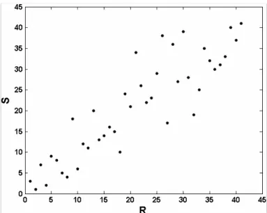
Once the univariate marginal distributions are known, the first step consists of study-ing the dependence between the two random variables: peak and volume. The scatter plot of the pairs (R_i,S_i) of ranks derived from the data set shows a positive relation

5

of dependence between variables (Fig. 2). This fact is also supported by the Chi-plot (Fig. 3a) and the K-plot (Fig. 3b). In the former, the values are located above the up-per limit indicating positive dependence. In the latter, the values are plotted over the diagonal line, so positive interaction is also drawn.

The value of the Spearman’s rho (ρ) and Kendall’s tau (τ) rank based non-parametric

10

measures of dependence corroborate the results provided by the graphical information. The value of each dependence measure as well as its linked p-value are summarised in Table 3.

The set of copulas considered is classified into three classes: Archimedean copulas, extreme value copulas and other families. Ali-Mikhail-Haq, Clayton, Frank and Gumbel

15

copulas belong to the first class, while Galambos, H ¨usler-Reiss, and Tawn copula are part of the extreme value copulas family. The Gumbel copula also belongs to the sec-ond group. Farlie-Gumbel-Morgenstern and Plackett are included into the last class. The set of feasible copulas was reduced after testing the admissible range of depen-dence supported by each one using the Kendall’s tau value. As result,

Ali-Mikhail-20

Haq (τ∈[−0.1817, 1/3]), Tawn (τ∈[0, 0.4184]) and Farlie-Gumbel-Morgenstern cop-ula (τ∈[−2/9, 2/9]) were eliminated.

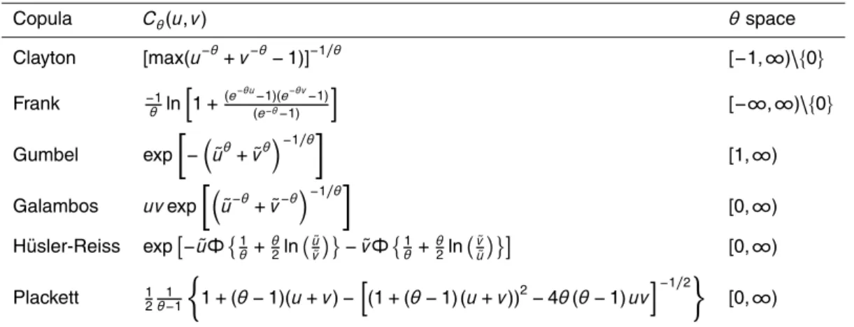
Copula functions and parameter space of the copulas selected in the study are pre-sented in Table 4. The parameter of the copulas is estimated using both rank based methods, the inversion of Kendall’s tau and the maximum pseudo-likelihood method.

25

(14)

HESSD

10, 557–596, 2013

Title Page

Tables Figures

◭ ◮

Back Close

Full Screen / Esc

Discussion

P

a

per

|

Dis

cussion

P

a

per

|

Discussion

P

a

per

|

Discussio

n

P

a

per

|

desirable. Besides, the standard error linked with the parameter of the extreme value copulas is the smallest.

100 000 synthetic pairs are generated from each copula. The scatter plot of the syn-thetic pairs transformed back into its original units using univariate marginal distribu-tions and the observed data are shown in Fig. 4. Only copulas whose parameter is

5

obtained by inversion of Kendall’s tau method are drawn. The figure shows that ex-treme value copulas (Gumbel, Galambos and H ¨usler-Reiss) are sharper in the upper right corner while the other copula models are more scattered in this area. This is so because extreme value copulas present positive dependence in the upper tail. The positive lower tail dependence of the Clayton copula can also be observed in the graph.

10

Extreme value copulas reproduce the behaviour of the data leaving the largest obser-vation on the edge of the simulated sample, while Clayton, Frank and Plackett copulas include this observation in the set of the generated sample, at the expense of an unde-sirable wider spread in the upper tail. A further analysis is needed to select the copula that best fits the data.

15

As expected, the generalized K-plot provides the same information for all of the extreme value copulas (Fig. 5). The distance between parametric (Kθn) and non-parametric estimate (Kn) ofK is greater for extreme value copulas than for the other

copula models. Consequently, this analysis shows that extreme value copulas are slightly worse in terms of fitting to the observed data.

20

In addition, the Sn goodness-of-fit test based on the empirical copula and its

as-sociated p-value based onN=_{10 000 parametric bootstrap samples (which are also}

included in Table 5) are estimated for each copula to select the suitable copulas in a formal way. This test shows a good behaviour for all copula families and makes a distinction among extreme value copulas. The results show that theS_n leads to better

25

(15)

HESSD

10, 557–596, 2013

Title Page

Tables Figures

◭ ◮

Back Close

Full Screen / Esc

Discussion

P

a

per

|

Dis

cussion

P

a

per

|

Discussion

P

a

per

|

Discussio

n

P

a

per

|

lower value of S_n and a suitable p-value), neither of the remaining copulas could be rejected considering the p-value.

Then, the upper tail dependence is analysed to take the behaviour of the copula model in the upper part of the distribution into account. The graphical analysis of the upper tail dependence is carried out based on the Chi-plot (Fig. 6). The analysis

in-5

dicates that upper tail dependence exists in the data set as the points located in the right edge show values diff_{erent from zero (independence). In addition, Table 6 shows}

the results of theλC_Uof the studied copulas. The coeffi_{cients were estimated using the}

copula parameter obtained by the inversion of Kendall’s tau method, as this method obtained better results. As Fig. 4 announced, only the extreme value copulas show

10

upper tail dependence. The remaining copulas show a null result, as they are not able to represent the upper tail dependence. The non-parametric estimator of the upper tail dependence coeffi_{cient obtained by means of Eq. (7), ˆ}_λCFG

U =0.749, is compared

with the upper tail dependence coeffi_{cient of each considered copula. As the estimator}

value is similar to the three values obtained for the extreme value copulas, it can be

15

considered that Gumbel, Galambos and H ¨usler-Reiss copulas reproduce suitably the dependence in the upper extreme.

The best copula should represent properly both the dependence structure of the peak and volume and the extreme events. Considering the whole tests, the Gumbel copula was selected as the best copula model. Although the best copula model based

20

on the goodness-of-fit test is the Frank copula, the Gumbel copula is the extreme value copula with the lower value of Sn and a suitable p-value. So, it takes into account

the upper tail dependence and represents properly the dependence structure between variables. Besides, as the Gumbel copula is also an Archimedean copula, it preserves the useful properties of this family.

25

(16)

HESSD

10, 557–596, 2013

Title Page

Tables Figures

◭ ◮

Back Close

Full Screen / Esc

Discussion

P

a

per

|

Dis

cussion

P

a

per

|

Discussion

P

a

per

|

Discussio

n

P

a

per

|

4.2 Joint return periods

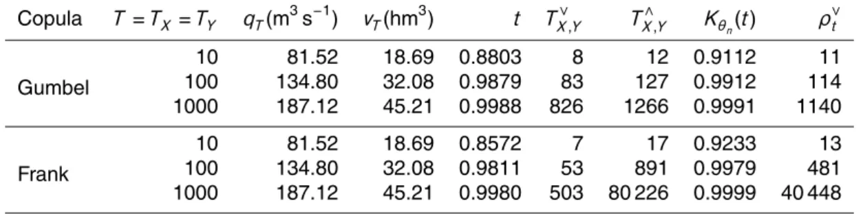
Firstly, a brief analysis is conducted to check the results of the copula selection by comparing the risk assumed depending on the selection of a copula model without upper tail dependence (Frank copula) and a copula model with upper tail dependence (Gumbel copula). The joint return periods T_X∨_,_Y (Eq. 8),T_X∧_,_Y (Eq. 9) and ρ∨_t (Eq. 11)

5

associated to the theoretical events with peak equal toq_T and volume equal tov_T for return periods (T) equal to 10, 100 and 1000 yr are estimated for both Gumbel and Frank copula. The results presented in Table 7 indicate that althoughT_X∨_,_Y linked to the Gumbel copula are higher for all the return periods,T_X∧_,_Y and theρ∨_t are much smaller. It can also be seen that the higher the return period, the larger the diff_{erences between}

10

joint return periods related to each copula. Therefore, the Frank copula underestimates the risk associated to the joint return periods T_X∧_,_Y and ρ∨_t. Thereby, not taking into consideration the upper tail dependence in joint extreme events modelling can lead to an underestimation of the risk (Poulin et al., 2007).

Therefore, once the Gumbel copula was selected as the best copula model, the joint

15

return periodsT_X∨_,_Y,T_X∧_,_Y andρ∨_t were calculated through it (Fig. 9).

4.3 Synthetic hydrograph generation

100 000 annual synthetic hydrographs were estimated by means of the 100 000 peak – volume pairs generated from the Gumbel copula. The set of hydrographs was routed through the reservoir, which was assumed to be uncontrolled for the sake of simplicity.

20

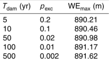
The frequency curve of the maximum water level reached was obtained for the spill-way real setup (an elevation of the spillspill-way crest of 889 m and a spillspill-way length of 12 m) (Fig. 8). Maximum water level quantiles for a given return period (WEmax)were

estimated easily from this frequency curve (Table 8). Return period curves in the peak-volume space regarding the risk to the dam were obtained as the hydrographs that lead

25

to a same water level WEmax. Thereby, Fig. 9 shows the comparison among the curves

(17)

HESSD

10, 557–596, 2013

Title Page

Tables Figures

◭ ◮

Back Close

Full Screen / Esc

Discussion

P

a

per

|

Dis

cussion

P

a

per

|

Discussion

P

a

per

|

Discussio

n

P

a

per

|

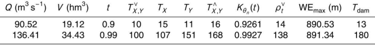
periodsT_X∨_,_Y,T_X∧_,_Y andρ∨_t. This graph provides useful information about observed and predicted events. It can be seen that the secondary return period curves are the most similar to the return period curves that represent the risk to the dam, as the way that they were calculated is analogous. The secondary return period is the probability that an event with a copula value higher thantoccurs, while the return period related to the

5

dam is calculated as the probability of exceeding a water level. As an example, Table 9 summarises this information for two specific events with a copula value of 0.9 and 0.99. The results fulfil the Eq. (10).

Once the diff_{erent curves were compared, a further analysis is carried out on the}

return period related to the risk to the dam, in order to assess its sensitivity. Figure 10

10

displays the return period curves for diff_{erent reservoir volumes given by reservoir}

el-evations of 879, 884 and 889 m and spillway lengths of 7, 12 and 17 m. It can be appreciated that the higher the reservoir volume, the more horizontal the curves, while the longer the spillway length, the steeper the curves. Thereby, the most horizontal curve is associated with the highest reservoir volume (E=_{889 m) and the shortest}

spill-15

way length (L=_{7 m), while the steepest curve is linked to the smallest reservoir volume}

(E=_{879 m) and the longest spillway length (}_L=_{17 m). This is caused by flood control}

properties in a reservoir: the higher the reservoir volume, the greater the capacity to store hydrograph water volume temporarily and, consequently, the higher the attenu-ation of the flood peak. In this case, the hydrographs that have more influence on the

20

risk to the dam, or the most dangerous hydrographs, are characterised by a high vol-ume. Consequently,Tdam is mostly given by the marginal return period of hydrograph

volumes (the curves are more horizontal). On the other hand, the smaller the reservoir volume, the lower the capacity to store water temporarily and the smaller the attenu-ation of the flood peak. In this case, the hydrographs that have more influence on the

25

risk to the dam are characterised by a high flood peak andTdam is mostly given by the

marginal return period of flood peaks (the curves are steeper).

(18)

HESSD

10, 557–596, 2013

Title Page

Tables Figures

◭ ◮

Back Close

Full Screen / Esc

Discussion

P

a

per

|

Dis

cussion

P

a

per

|

Discussion

P

a

per

|

Discussio

n

P

a

per

|

that lead to a higher maximum water level will have greater volumes andTdamis mostly

given by the marginal return period of hydrograph volumes.

5 Conclusions

In the present paper a Monte Carlo procedure to compare the probability of occurrence of a flood with an empirical return period linked to the risk to the dam was developed.

5

For that purpose a bivariate flood frequency analysis of flood peak and volume via a copula model was conducted. The Gumbel copula was found to be the best copula after taking into account the upper tail dependence of the data set. A set of synthetic flood hydrographs was generated from the fitted Gumbel copula and was routed through the Santillana reservoir to obtain the maximum water level reached during the

rout-10

ing, as the water lever was used as a surrogate of the hydrological risk to the dam. Curves that represent the risk to the dam were obtained as the probability of exceed-ing a water level. Joint return period curves were also estimated via the copula model. Comparison between both curves for diff_{erent return periods was carried out. Finally, a}

sensitivity analysis of the empirical return period curves related to the risk to the dam

15

was conducted considering diff_{erent reservoir volumes and spillway lengths.}

The results show that tail dependence should be considered in the copula selection to avoid hydrological risk underestimation. The secondary return period curves turned out to be the most similar to the empirical return period curves that represent the risk to the dam, as the way that they are calculated is analogous. This results support the

20

use of the secondary return period in dam design. However, in addition to using the secondary return period, flood hydrographs should also be routed to improve the esti-mation of the risk of dam overtopping, as there are diff_{erences among return periods.}

It was appreciated that as the available flood control volume increases, the empirical return period curves are more dependent on volume (the slope of the return period

25

(19)

HESSD

10, 557–596, 2013

Title Page

Tables Figures

◭ ◮

Back Close

Full Screen / Esc

Discussion

P

a

per

|

Dis

cussion

P

a

per

|

Discussion

P

a

per

|

Discussio

n

P

a

per

|

return period curves becomes steeper). Thereby, although a previous bivariate analysis is always necessary, there are cases in which a univariate return period analysis could be considered. It is also needed to emphasise that the shape of the curves depend on the reservoir volume and spillway length, but also on the hydrograph magnitude, given by soil properties, rainfall and physiographic characteristics of the basin.

5

In conclusion, comparison between bivariate return period curves that represent the risk of dam overtopping and bivariate joint return period curves that represent the prob-ability of occurrence of a flood event provides valuable information about flood control processes in the reservoir. In addition, this study could be replicated in terms of risk of downstream damages. Therefore, the proposed methodology can procure useful

10

information to estimate the Design Flood Hydrograph.

Acknowledgements. This work has been supported by the Carlos Gonz ´alez Cruz Foundation

and the project MODEX- Physically-based modelling of extreme hydrologic response under a probabilistic approach. Application to Dam Safety Analysis (CGL2011-22868), funded by the Spanish Ministry of Science and Innovation (now the Ministry of Economy and Competitive-15

ness). The authors are also grateful for the financial contribution made by the COST Office grant ES0901 “European procedures for flood frequency estimation (FloodFreq)”.

References

Abberger, K.: A simple graphical method to explore tail-dependence in stock-return pairs, Ap-plied Financial Economics, 15, 43–51, 2005.

20

Chebana, F. and Ouarda, T.: Multivariate quantiles in hydrological frequency analysis, Environ-metrics, 22, 63–78, 2011.

Chowdhary, H., Escobar, L. A., and Singh, V. P.: Identification of suitable copulas for bivariate frequency analysis of flood peak and flood volume data, Hydrol. Res., 42, 193–216, 2011. De Michele, C., Salvadori, G., Canossi, M., Petaccia, A., and Rosso, R.: Bivariate statistical 25

approach to check adequacy of dam spillway, J. Hydrol. Eng., 10, 50–57, 2005.

(20)

HESSD

10, 557–596, 2013

Title Page

Tables Figures

◭ ◮

Back Close

Full Screen / Esc

Discussion

P

a

per

|

Dis

cussion

P

a

per

|

Discussion

P

a

per

|

Discussio

n

P

a

per

|

Fisher, N. I. and Switzer, P.: Chi-Plots for Assessing Dependence, Biometrika, 72, 253–265, 1985.

Fisher, N. I. and Switzer, P.: Graphical assessment of dependence: Is a picture worth 100 tests?, Am. Stat., 55, 233–239, 2001.

Frahm, G., Junker, M., and Schmidt, R.: Estimating the tail-dependence coefficient: Properties 5

and pitfalls, Insur. Math. Econ., 37, 80–100, 2005.

Genest, C. and Boies, J. C.: Detecting dependence with Kendall plots, Am. Stat., 57, 275–284, 2003.

Genest, C. and Favre, A.-C.: Everything you always wanted to know about copula modeling but were afraid to ask, J. Hydrol. Eng., 12, 347–368, 2007.

10

Genest, C. and R ´emillard, B.: Validity of the parametric bootstrap for goodness-of-fit testing in semiparametric models, Ann. I. H. Poincare-Pr., 44, 1096–1127, 2008.

Genest, C. and Rivest, L.: Statistical Inference Procedures for Bivariate Archimedean Copulas, J. Am. Stat. Assoc., 88, 1034–1043, 1993.

Genest, C., Quessy, J. F., and R ´emillard, B.: Goodness-of-fit Procedures for Copula Models 15

Based on the Probability Integral Transformation, Scand. J. Stat, 33, 337–366, 2006. Genest, C., R ´emillard, B., and Beaudoin, D.: Goodness-of-fit tests for copulas: A review and a

power study, Insur. Math. Econ., 44, 199–213, 2009.

Grimaldi, S. and Serinaldi, F.: Asymmetric copula in multivariate flood frequency analysis, Adv. Water Resour., 29, 1155–1167, 2006.

20

Joe, H.: Multivariate model and dependence concepts, Chapman and Hall, London, 1997. Joe, H. and Xu, J. J.: The estimation method of Inference functions for margins for multivariate

models, Technical Rep. 166, Department of Statistics, University of British Colombia, 1996. Kim, G., Silvapulle, M. J., and Silvapulle, P.: Comparison of semiparametric and parametric

methods for estimating copulas, Comput. Stat. Data An., 51, 2836–2850, 2007. 25

Klein, B., Pahlow, M., Hundecha, Y., and Schumann, A.: Probability analysis of hydrological loads for the design of flood control systems using copulas, J. Hydrol. Eng., 15, 360–369, 2010.

Mediero, L., Jim ´enez- ´Alvarez, A., and Garrote, L.: Design flood hydrographs from the re-lationship between flood peak and volume, Hydrol. Earth Syst. Sci., 14, 2495–2505, 30

doi:10.5194/hess-14-2495-2010, 2010.

(21)

HESSD

10, 557–596, 2013

Title Page

Tables Figures

◭ ◮

Back Close

Full Screen / Esc

Discussion

P

a

per

|

Dis

cussion

P

a

per

|

Discussion

P

a

per

|

Discussio

n

P

a

per

|

Nelsen, R. B.: An introduction to copulas, Springer, New York, 1999.

Poulin, A., Huard, D., Favre, A.-C., and Pugin, S.: Importance of tail dependence in bivariate frequency analysis, J. Hydrol. Eng., 12, 394–403, 2007.

Salvadori, G. and De Michele, C.: Frequency analysis via copulas: Theoretical aspects and applications to hydrological events, Water Resour. Res., 40, 1–17, 2004.

5

Salvadori, G., De Michele, C., Kottegoda, N. T., and Rosso, R.: Extremes in nature. An approach using copulas, Springer, Dordrecht, The Netherlands, 2007.

Serinaldi, F.: Analysis of inter-gauge dependence by Kendall’sτK, upper tail dependence co-efficient, and 2-copulas with application to rainfall fields, Stoch. Env. Res. Risk. A., 22, 671– 688, 2008.

10

Serinaldi, F. and Grimaldi, S.: Fully nested 3-copula: procedure and application on hydrological data, J. Hydrol. Eng., 12, 420–430, 2007.

Shiau, J., Wang, H., and Tsai, C.: Bivariate frequency analysis of floods using copulas, J. Am. Water Resour. As., 42, 1549–1564, 2006.

Sklar, A.: Fonctions de r ´epartition `a n dimensions et leurs marges, Publ. Inst. Stat. Univ. Paris, 15

8, 229–231, 1959.

Zhang, L. and Singh, V. P.: Bivariate flood frequency analysis using the copula method, J. Hydrol. Eng., 11, 150–164, 2006.

Zhang, L. and Singh, V. P.: Trivariate flood frequency analysis using the Gumbel-Hougaard copula, J. Hydrol. Eng., 12, 431–439, 2007.

(22)

HESSD

10, 557–596, 2013

Title Page

Tables Figures

◭ ◮

Back Close

Full Screen / Esc

Discussion

P

a

per

|

Dis

cussion

P

a

per

|

Discussion

P

a

per

|

Discussio

n

P

a

per

|

Table 1.Santillana reservoir characteristics: drainage area (A), volume up to the spillway crest (Vol), flooded area at the spillway crest height (S) and elevation of the spillway crest (E).

A(km2) Vol (hm3) S(km2) E (m)

(23)

HESSD

10, 557–596, 2013

Title Page

Tables Figures

◭ ◮

Back Close

Full Screen / Esc

Discussion

P

a

per

|

Dis

cussion

P

a

per

|

Discussion

P

a

per

|

Discussio

n

P

a

per

|

Table 2.Location parameter (µ) and scale parameter (σ) of Gumbel distributions for the vari-ables of peak (Q) and volume (V).

Variable µ σ

Q 30.47 22.69

(24)

HESSD

10, 557–596, 2013

Title Page

Tables Figures

◭ ◮

Back Close

Full Screen / Esc

Discussion

P

a

per

|

Dis

cussion

P

a

per

|

Discussion

P

a

per

|

Discussio

n

P

a

per

|

Table 3. Rank based non-parametric measures of dependence: Spearman’s rho (ρ) and Kendall’s tau (τ).

Dependence measure Value p-value

ρ 0.8899 1.82e-08

(25)

HESSD

10, 557–596, 2013

Title Page

Tables Figures

◭ ◮

Back Close

Full Screen / Esc

Discussion

P

a

per

|

Dis

cussion

P

a

per

|

Discussion

P

a

per

|

Discussio

n

P

a

per

|

Table 4.Copula functions and parameter space of the considered copulas.

Copula C_θ(u,v) θspace Clayton [max(u−θ+_v−θ₋_1)]−1/θ _[₋_1,_∞₎_\{₀_}

Frank −_θ1lnh1+(e−θu−1)(e−θv−1)

(e−θ₋₁₎

i

[−∞,∞)\{0}

Gumbel exp

−u˜θ+_v_˜θ−1/θ

[1,∞)

Galambos uvexp

˜

u−θ+_v_˜−θ−1/θ

[0,∞) H ¨usler-Reiss exp

−u˜Φ1 θ+θ2ln

˜ u ˜

v −v˜Φ

1 θ+θ2ln

˜ v ˜

u [0,∞)

Plackett 1 2

1 θ−1

1+₍_θ₋₁₎₍_u+_v₎₋h₍₁+₍_θ₋_{1) (}_u+_v₎₎2₋₄_θ₍_θ₋₁₎_uvi−1/2

[0,∞)

(26)

HESSD

10, 557–596, 2013

Title Page

Tables Figures

◭ ◮

Back Close

Full Screen / Esc

Discussion

P

a

per

|

Dis

cussion

P

a

per

|

Discussion

P

a

per

|

Discussio

n

P

a

per

|

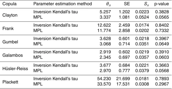
Table 5.Estimated value of the copula parameter (θ_n), copula parameter standard error (SE), Cram ´er-von Mises goodness-of-fit test (S_n) and p-value calculated based onN=10 000 para-metric bootstrap samples, according to the parameter estimation method.

Copula Parameter estimation method θ_n SE S_n p-value

Clayton Inversion Kendall’s tau_MPL 5.257_3.337 1.202_1.081 0.0223_0.0524 0.3828_0.0565

Frank Inversion Kendall’s tau_MPL 12.622_11.774 2.459_2.858 0.0174_0.0202 0.8402_0.7332

Gumbel Inversion Kendall’s tau_MPL 3.628_3.068 0.601_0.714 0.0218_0.0351 0.3967_0.0649

Galambos Inversion Kendall’s tau_MPL 2.919_2.345 0.602_0.697 0.0219_0.0357 0.3910_0.0603

H ¨usler-Reiss Inversion Kendall’s tau_MPL 3.677_2.970 0.684_0.777 0.0221_0.0379 0.3663_0.0568

(27)

HESSD

10, 557–596, 2013

Title Page

Tables Figures

◭ ◮

Back Close

Full Screen / Esc

Discussion

P

a

per

|

Dis

cussion

P

a

per

|

Discussion

P

a

per

|

Discussio

n

P

a

per

|

Table 6.Upper tail dependence coefficient of the considered copulas.

Copula λC_U(θ) θ_n λˆC_U

Clayton 0 5.257 0

Frank 0 12.622 0

Gumbel 2−21/θ 3.628 0.789

Galambos 2−1/θ 2.919 0.789

H ¨usler-Reiss 2−2Φ₁

θ 3.677 0.786

Plackett 0 54.230 0

(28)

HESSD

10, 557–596, 2013

Title Page

Tables Figures

◭ ◮

Back Close

Full Screen / Esc

Discussion

P

a

per

|

Dis

cussion

P

a

per

|

Discussion

P

a

per

|

Discussio

n

P

a

per

|

Table 7. Comparison between joint return periods associated to the theoretical events with peak equal toq_T and volume equal tov_T forT =10, 100 and 1000 yr.

Copula T=_T_X =_T_Y _q_T(m3s−1) v_T(hm3) t T_X∨_,_Y T_X∧_,_Y K_θ

n(t) ρ

∨

t

Gumbel

10 81.52 18.69 0.8803 8 12 0.9112 11

100 134.80 32.08 0.9879 83 127 0.9912 114

1000 187.12 45.21 0.9988 826 1266 0.9991 1140

Frank

10 81.52 18.69 0.8572 7 17 0.9233 13

100 134.80 32.08 0.9811 53 891 0.9979 481

(29)

HESSD

10, 557–596, 2013

Title Page

Tables Figures

◭ ◮

Back Close

Full Screen / Esc

Discussion

P

a

per

|

Dis

cussion

P

a

per

|

Discussion

P

a

per

|

Discussio

n

P

a

per

|

Table 8.Maximum water level reached for different return periods (WE_max) associated to the probability of exceeding a water level forE=889 m and L=12m.

T_dam (yr) p_exc WE_max(m)

5 0.2 890.21

10 0.1 890.46

50 0.02 890.98

100 0.01 891.17

(30)

HESSD

10, 557–596, 2013

Title Page

Tables Figures

◭ ◮

Back Close

Full Screen / Esc

Discussion

P

a

per

|

Dis

cussion

P

a

per

|

Discussion

P

a

per

|

Discussio

n

P

a

per

|

Table 9.Example of comparison among return periods. Two simulated events with a copula value of 0.9 and 0.99 are considered. All return periods are expressed in years.

Q(m3s−1) V (hm3) t T_X∨_,_Y T_X T_Y T_X∧_,_Y K_θ

n(t) ρ

∨

t WEmax(m) Tdam

90.52 19.12 0.9 10 15 11 16 0.9261 14 890.53 13

(31)

HESSD

10, 557–596, 2013

Title Page

Tables Figures

◭ ◮

Back Close

Full Screen / Esc

Discussion

P

a

per

|

Dis

cussion

P

a

per

|

Discussion

P

a

per

|

Discussio

n

P

a

per

|

(32)

HESSD

10, 557–596, 2013

Title Page

Tables Figures

◭ ◮

Back Close

Full Screen / Esc

Discussion

P

a

per

|

Dis

cussion

P

a

per

|

Discussion

P

a

per

|

Discussio

n

P

a

per

|

(33)

HESSD

10, 557–596, 2013

Title Page

Tables Figures

◭ ◮

Back Close

Full Screen / Esc

Discussion

P

a

per

|

Dis

cussion

P

a

per

|

Discussion

P

a

per

|

Discussio

n

P

a

per

|

(34)

HESSD

10, 557–596, 2013

Title Page

Tables Figures

◭ ◮

Back Close

Full Screen / Esc

Discussion

P

a

per

|

Dis

cussion

P

a

per

|

Discussion

P

a

per

|

Discussio

n

P

a

per

|

(35)

HESSD

10, 557–596, 2013

Title Page

Tables Figures

◭ ◮

Back Close

Full Screen / Esc

Discussion

P

a

per

|

Dis

cussion

P

a

per

|

Discussion

P

a

per

|

Discussio

n

P

a

per

|

K Fig. 5.Comparison between parametric (K_θ

n) and non-parametric (Kn) estimate ofK,

(36)

HESSD

10, 557–596, 2013

Title Page

Tables Figures

◭ ◮

Back Close

Full Screen / Esc

Discussion

P

a

per

|

Dis

cussion

P

a

per

|

Discussion

P

a

per

|

Discussio

n

P

a

per

|

(37)

HESSD

10, 557–596, 2013

Title Page

Tables Figures

◭ ◮

Back Close

Full Screen / Esc

Discussion

P

a

per

|

Dis

cussion

P

a

per

|

Discussion

P

a

per

|

Discussio

n

P

a

per

|

(38)

HESSD

10, 557–596, 2013

Title Page

Tables Figures

◭ ◮

Back Close

Full Screen / Esc

Discussion

P

a

per

|

Dis

cussion

P

a

per

|

Discussion

P

a

per

|

Discussio

n

P

a

per

|