A past discharges assimilation system for ensemble streamflow forecasts over France – Part 1: Description and validation of the assimilation system

(1)

HESSD

7, 2413–2453, 2010

Description and validation of the assimilation system

G. Thirel et al.

Title Page

Abstract Introduction

Conclusions References

Tables Figures

◭ ◮

Back Close

Full Screen / Esc

Printer-friendly Version

Interactive Discussion

Hydrol. Earth Syst. Sci. Discuss., 7, 2413–2453, 2010 www.hydrol-earth-syst-sci-discuss.net/7/2413/2010/ © Author(s) 2010. This work is distributed under the Creative Commons Attribution 3.0 License.

Hydrology and Earth System Sciences Discussions

This discussion paper is/has been under review for the journal Hydrology and Earth System Sciences (HESS). Please refer to the corresponding final paper in HESS if available.

A past discharges assimilation system for

ensemble streamflow forecasts over

France – Part 1: Description and

validation of the assimilation system

G. Thirel1,2, E. Martin1, J.-F. Mahfouf1, S. Massart3, S. Ricci3, and F. Habets4

1

CNRM/GAME (M ´et ´eo-France, CNRS) URA 1357, Toulouse, France

2

IES, Joint Research Centre, European Commission, Ispra, Italy

3

URA CNRS/CERFACS No. 1875, Toulouse, France

4

UMR Sisyphe, UPMC, ENSMP, CNRS, Paris, France

Received: 6 April 2010 – Accepted: 6 April 2010 – Published: 22 April 2010

Correspondence to: G. Thirel (guillaume.thirel@jrc.ec.europa.eu)

(2)

HESSD

7, 2413–2453, 2010

G. Thirel et al.

Title Page

Tables Figures

◭ ◮

Back Close

Full Screen / Esc

Abstract

Two Ensemble Streamflow Prediction Systems (ESPSs) have been set up at M ´et ´eo-France. They are based on the French SIM distributed hydrometeorological model. A deterministic analysis run of SIM is used to initialize the two ESPSs. In order to obtain a better initial state, a past discharges assimilation system has been implemented into 5

this analysis SIM run, using the Best Linear Unbiased Estimator (BLUE). Its role is to improve the model soil moisture by using observed streamflows in order to better simulate streamflow. The skills of the assimilation system were assessed for a 569-day period on six different configurations, including two different physics schemes of the model (the use of an exponential profile of hydraulic conductivity or not) and, for 10

each one, three di_fferent ways of considering the model soil moisture in the BLUE state variables. Respect of the linearity hypothesis of the BLUE was verified by assessing of the impact of iterations of the BLUE. The configuration including the use of the exponential profile of hydraulic conductivity and the combination of the moisture of the two soil layers in the state variable showed a significant improvement of streamflow 15

simulations. It led to a significantly better simulation than the reference one, and the lowest soil moisture corrections. These results were confirmed by the study of the impacts of the past discharge assimilation system on a set of 49 independent stations.

1 Introduction

Improving streamflow forecasting is a key issue for preserving human lives and mate-20

rial, and for monitoring water resources. Much effort has been put into coupling Land Surface Models (LSMs) with hydrological models to improve the simulation of physical processes, and into increasing the spatial resolution of these models. Unfortunately, not all hydrological processes are easily predictable. In particular, hydrology is very dependent on precipitation, which is a highly stochastic phenomenon, and questions 25

(3)

HESSD

7, 2413–2453, 2010

G. Thirel et al.

Title Page

Tables Figures

◭ ◮

Back Close

Full Screen / Esc

One attempt to address the difficulty of precipitation prediction involves the use of meteorological ensemble prediction. This kind of prediction, relying mostly on meteo-rological ensemble forecasts forcing an hydmeteo-rological model, tends to give better scores on streamflows than deterministic predictions. Much research is underway on this sub-ject, such as the Hydrologic Ensemble Prediction EXperiment (HEPEX) (Schaake et al. 5

(2006), and see the website http://hydis8.eng.uci.edu/hepex) which “brings together hydrological and meteorological communities from around the globe to build a research project focused on advancing probabilistic hydrologic forecast techniques”.

In Europe, the European Flood Alert System (EFAS) prototype (Ramos et al., 2007) is based on the European Centre for Medium-Range Weather Forecasts (ECMWF) 10

Ensemble Prediction System (EPS) (Chessa and Lalaurette, 2001; Buizza et al., 2007) and sends alerts to European countries.

In France, two Ensemble Streamflow Prediction Systems (ESPSs) have been set up using the ECMWF EPS (Rousset-Regimbeau et al., 2007) and the M ét éo-France EPS, “Pr évision d’Ensemble Action de Recherche Petite Echelle Grande Echelle” (PEARP) 15

and have been compared using statistical scores over a long period (Thirel et al., 2008). Data assimilation combines physical and observational information on a system in order to provide a better description of the system. The benefit of data assimilation has already been amply demonstrated in meteorology and oceanography over the past decades, where it helps to provide initial conditions for numerical prediction. However 20

its use in the field of hydrology is more recent. Data assimilation in hydrological mod-elling can be used for three main purposes: improving soil moisture states, improving streamflow predictions, and optimizing models parameters. It can be carried out by analysing soil moisture, or/and streamflow data.

For example, Reichle et al. (2002) assessed the performance of an Extended Kalman 25

(4)

HESSD

7, 2413–2453, 2010

G. Thirel et al.

Title Page

Tables Figures

◭ ◮

Back Close

Full Screen / Esc

in the Mississippi River basin. Aubert et al. (2003) developed an EnKF assimilation system for improving streamflow prediction over a Seine river sub-basin. Clark et al. (2008) used the EnKF in which states in a distributed hydrological model were updated by means of streamflow observations. They demonstrated that the standard imple-mentation of the EnKF was inappropriate because of non-linear relationships between 5

model states and observations and that transforming streamflow into log space be-fore computing error covariances as well as using a variant of the EnKF not requiring perturbed observations improved filter performance.

So far, few operational applications of such assimilation systems exist. Promising work was done by Komma et al. (2008) which implemented an EnKF for an Austrian 10

basin, for time flood forecasting. This system adjusts soil moisture for better real-time streamflows forecasting. Seo et al. (2009) give details of an operational vari-ational assimilation (VAR) of streamflow, precipitation and potential evaporation data into lumped soil moisture accounting and routing models operating at a 1-h timestep.

This paper presents the work performed using assimilation to update soil mois-15

ture states of the M ´et ´eo-France hydrometeorological model SAFRAN-ISBA-MODCOU (SIM), in order to improve streamflow predictions. Various soil moisture states and soil water physics are assessed in this framework. The originality and difficulty of this study lies in the fact that the data assimilation system is applied over a distributed model, for embedded station networks, and for all of France.

20

The SIM hydrometeorological model is described in Sect. 2. Then the coupler soft-ware PALM, in which the assimilation system was implemented, and the BLUE assimi-lation method are described in Sect. 3. Section 4 presents the design and methodology of the assimilation system. The results obtained by the assimilation system on the SIM analysis suite with different settings are presented and discussed in Sect. 5, and a 25

(5)

HESSD

7, 2413–2453, 2010

G. Thirel et al.

Title Page

Tables Figures

◭ ◮

Back Close

Full Screen / Esc

2 The SAFRAN-ISBA-MODCOU hydrometeorological model

Both the analysis suite and the hydrological forecasts are based on the SAFRAN-ISBA-MODCOU hydrometeorological suite. This suite is composed of three independent models: SAFRAN, ISBA and MODCOU.

SAFRAN (Syst ème d’Analyse Fournissant des Renseignements Atmosph ériques à

5

la Neige, an analysis system that provides atmospheric data to a snow model) is a near-surface meteorological analysis system (Durand et al., 1993). It combines teorological model outputs with surface observations to produce hourly values of me-teorological variables. SAFRAN provides eight parameters (10-m wind speed, 2-m relative humidity, 2-m air temperature, total cloud cover, incoming solar and atmo-10

spheric/terrestrial radiation, snowfall and rainfall) interpolated over France on the ISBA 8-km grid. Recently, Quintana Segu´ı et al. (2008) assessed the quality of SAFRAN against observations, showing that most of the parameters are well reproduced by SAFRAN.

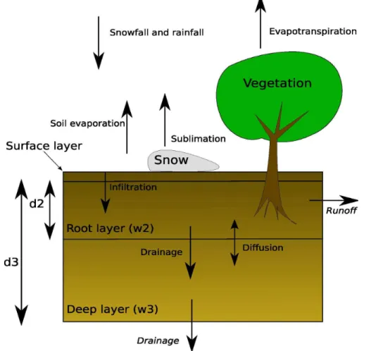
ISBA (Interactions between Soil, Biosphere and Atmosphere, Noilhan and Planton 15

(1989), Noilhan and Mahfouf, 1996) is an LSM developed at M ét éo-France. It simulates water and energy fluxes between the soil and the atmosphere (Fig. 1) with a simple parameterization. ISBA is used in research, numerical weather prediction and climate modelling at M ét éo-France. For hydrological applications (i.e. the SIM suite), the three-layer force-restore version is used (Boone et al., 1999) together with an explicit snow 20

model (Boone and Etchevers, 2001) (Fig. 1). A subgrid runoffscheme (Habets et al., 1999a) and a subgrid drainage scheme (Habets et al., 1999b) have been implemented to tackle the issue of physical processes occuring at smaller scales than the 8-km ISBA grid. ISBA simulates the runoffthrough the Dunne mechanism over saturation. For soil moisture under the saturation point, the subgrid runoff is activated, its amount being 25

(6)

HESSD

7, 2413–2453, 2010

G. Thirel et al.

Title Page

Tables Figures

◭ ◮

Back Close

Full Screen / Esc

for more details about the runo_ffand drainage processes). Recently, Quintana Segu´_ıet al. (2009) introduced an optional exponential profile of hydraulic conductivity in the soil into ISBA, resulting in a better simulation of river discharges. This feature is intended to reduce the drainage flux to the river, which was too high at early times after heavy rains, by spreading the flux over time.

5

MODCOU (MOD èle COUpl é (Coupled Model), Ledoux et al., 1989) is a distributed hydrogeological model. It simulates the spatial and temporal evolution of two aquifers (located over the Seine and Rh ône basins) using a diffusivity equation. The interaction between these aquifers and the rivers is described, and the soil water is routed towards and into the rivers with a simple isochronism algorithm. Streamflows are produced with 10

a 3-h time step, but used and validated at a 1-day time step. The ISBA drainage and runoffvariables are used by MODCOU in the SIM suite (corresponding to drainage and runo_ffvariables in italics in Fig. 1).

SIM was first validated for three large French river basins: the Rh ˆone (Etchevers et al., 2001), the Adour-Garonne (Morel, 2003) and the Seine (Rousset et al., 2004). 15

Then, SIM was extended and validated over the whole of France (Habets et al., 2008), supplying realistic water and energy budgets, streamflows, aquifer levels and snowpack simulations. Around 900 streamflow stations are simulated over France. SIM has been running operationally once a day at M ´et ´eo-France since 2003 in an analysis mode. It is used for soil water reports and as a tool for the French national flood alert services, 20

for both its streamflow and soil moisture outputs.

Based on the SIM suite, two ensemble hydrological forecast systems have been built, using the ECMWF EPS (Rousset-Regimbeau et al., 2007) and the PEARP EPS (Thirel et al., 2008). The initial soil, river and aquifer states of these two systems come from the operational analysis SIM suite described above. However, this suite is not perfect 25

(7)

HESSD

7, 2413–2453, 2010

G. Thirel et al.

Title Page

Tables Figures

◭ ◮

Back Close

Full Screen / Esc

That is why a streamflow assimilation system has been set up in SIM, in order to improve streamflow predictions. The assimilation system will rely on modifying the soil moisture of ISBA because this variable is very relevant to the river flow in the medium term. Directly modifying the amount of water in the rivers would only tackle the short term and modifying the aquifer layers would only concern the Seine and Rh ˆone basins. 5

The assimilation system and its impacts on the SIM suite forced by analysed data are described in the following section.

3 Tools used for the data assimilation system

The streamflow assimilation system was implemented in the PALM coupling software, and a linear estimation (BLUE) was used to optimize the ISBA soil moisture.

10

3.1 The PALM coupling software

PALM (Parallel Assimilation with a Lot of Modularity; Lagarde et al., 2001) is a dynamic parallel coupler implemented by the CERFACS (European Centre for Research and Advanced Training in Scientific Computation). PALM was written because the CER-FACS was given the task of designing software that could handle the numerous meth-15

ods of data assimilation needed for the oceanographic project MERCATOR (Brasseur et al., 2005). The specificities of PALM are a dynamic launch of the coupled compo-nents, independence of the various components which allows full modularity, and a set of standard algebra libraries (Fouilloux and Piacentini, 1999; Buis et al., 2006). More-over, PALM is particularly well adapted to the M ´et ´eo-France NEC supercomputer plat-20

form, and takes advantage of its cluster structure requiring little parallelization knowl-edge from the user.

(8)

HESSD

7, 2413–2453, 2010

G. Thirel et al.

Title Page

Tables Figures

◭ ◮

Back Close

Full Screen / Esc

3.2 The Best Linear Unbiased Estimator (BLUE) method

The BLUE method is the analysis operator used for the streamflow assimilation system. This method assumes that background and observation errors are unbiased and non-correlated. The analysis statexa is an estimation of the true state xt, such thatxa=

xt+ǫa, whereǫais the analysis error. The BLUE relies on minimizingTr(A) with respect 5

toK(Bouttier and Courtier, 1999), withA, the analysis error covariance matrix, defined as follows:

A=(I−KH)B(I−KH)T+KRKT, (1)

whereRandBrepresent the observation and background error covariance matrices, respectively,His the Jacobian matrix of the observation operatorH computed around 10

the background state xb, and K is a linear operator (the gain matrix) to be defined. Bouttier and Courtier (1999) showed that:

xa=xb+K(y₀− H(xb)), (2)

which highlights the fact that the data assimilation system gives a correction applied to the background statexb.y0is the observation vector andH(x

b

) the model equivalent 15

of the observations. The value ofKminimizingTr(A) is:

K=(B−1+HTR−1H)−1HTR−1, (3)

The H, R, y0 and H(x b

) quantities can contain information at several time steps, depending on the size of the assimilation window. In that way, the BLUE analysis tries to find the state at the beginning of the assimilation window (xa) that will result in the 20

simulation closest to a set of available observations, given an a priori state (xb) for this initial condition. The BLUE method was chosen because of the small size of the observation and state variables, which made it possible to compute the exact solution for theKmatrix. It relies on the assumption that the operatorH is not too non-linear over the [xb,xa] interval.

(9)

HESSD

7, 2413–2453, 2010

G. Thirel et al.

Title Page

Tables Figures

◭ ◮

Back Close

Full Screen / Esc

In the case of our application, the streamflows are assumed to be inexact, mostly because of soil moisture errors in ISBA. Thus the ISBA soil moisture is chosen to be the variable state (xband xavariables) of the optimization process. The observations (y0) used to correct soil moisture errors are streamflow observations. Consequently,B represents ISBA soil moisture error statistics andRrepresents observed streamflows 5

error statistics. H(xb) stands for streamflows computed by the SIM suite using the background soil moisturexb. H represents the model suite ISBA-MODCOU andHis its tangent linear version, computed around a reference often chosen asxb.

4 Streamflow assimilation methodology

The originality of the present streamflow assimilation system is that it is applied to a 10

distributed hydrometeorological model over the whole of France. Therefore, a wide range of basins (large or small, contrasted or not) and meteorological conditions are encompassed. Moreover, single basins and embedded basin networks are assimilated simultaneously. In the following, we show how some di_fficulties associated with these features were overcome.

15

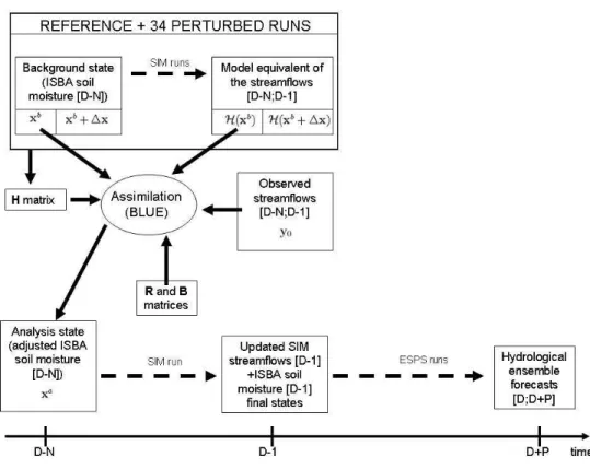
4.1 Principle of the assimilation process for SIM

The principle of the assimilation process is shown in Fig. 2 for anN-day time window, initializing ensemble forecasts lastingP+1 days and beginning on day (D).

The background state xb is the initial ISBA soil moisture state at day (D−N). The innovation vector is the difference between the observed streamflows and the simu-20

(10)

HESSD

7, 2413–2453, 2010

G. Thirel et al.

Title Page

Tables Figures

◭ ◮

Back Close

Full Screen / Esc

the background statexbwith small perturbations.

Then, BLUE uses all these elements to identify the analysis soil moisture state. The (D−N) background soil moisture is corrected by this analysis state, and SIM is integrated over the [D−N;D−1] time window. This integration provides soil moisture and river initial states for performing ensemble streamflow forecasts from day (D) to 5

day (D+P).

The assimilation process can be re-iterated after a delay of at leastNdays so as not to use the same streamflow observations several times.

4.2 Selection of gauge stations for observations

The streamflow observations come from the data collected by the “Banque Hydro” 10

over a network of approximately 3500 river gauge stations . This French database is available online at the following website: http://www.hydro.eaufrance.fr/. The stations simulated by SIM (≈900) all correspond to real gauge stations present in the “Banque Hydro” database. A set of 186 relevant gauge stations (good quality of streamflow measurements and SIM results) was selected for assimilation. Thus the size of the 15

variable state vector was 186. The discharge observations are available daily, and are daily-averaged values.

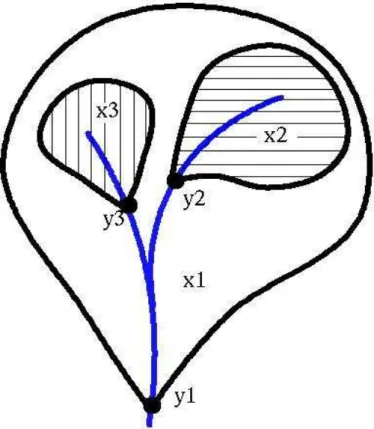
In order to respect the river structures and to deal with dependencies between sub-basins, all the stations were sorted into river “trees” (main basins) in which the bases were the down stream station (base station) and the “branches” were its upstream sub-20

stations (see an example in Fig. 3). The number of stations in a tree ranged from one (independent basins) to 34 (the Loire main basin).

4.3 State variable definitions

The state variable of the assimilation system is the soil moisture of SIM. In SIM, which includes the ISBA-3L version of ISBA (Boone et al., 1999), the soil is divided into three 25

(11)

HESSD

7, 2413–2453, 2010

G. Thirel et al.

Title Page

Tables Figures

◭ ◮

Back Close

Full Screen / Esc

layer (1-cm deep on average) is part of the root layer and has no impact on streamflows (this layer is mainly used to determine the surface humidity for bare soil evaporation), so the root- and deep- layers moisture are the only relevant state variables. Three definitions of the state variable were considered. Ifw2andw3(a different value for each ISBA grid mesh) stand for the soil water content (in m3/m3) of the root and deep layers, 5

respectively (see Fig. 1), andd2 and d3−d2 are their corresponding thicknesses, the elements of the first state variable are:

xi=

X

sub−basini

d2·w2+(d3−d2)·w3

d3

(4)

The second method only used the root-layer water content:

x_i= X

sub−basini

w2 (5)

10

The last method considered each soil layer water content separately:

 



x_i₌ P

sub−basini

w2, if 1≤i≤186

xi= P

sub−basin (i−186)

w3,if 187≤i≤372

(6)

The size of this last state variable is twice that of the previously described state

vari-ables. Each P

sub−basinı

sign indicates that the sum is taken over the sub-basini,

exclud-ing meshes belongexclud-ing to another upstream assimilated sub-basin. 15

(12)

HESSD

7, 2413–2453, 2010

G. Thirel et al.

Title Page

Tables Figures

◭ ◮

Back Close

Full Screen / Esc

is given in Eq. (7) for an ISBA mesh included in theith assimilated basin (for Eqs. 4 or 5):

w_2,3a =w_2,3b ∗xa_i/xb_i (7)

4.4 Practical implementation

In the following, equations and matrices are illustrated for the simplest case of a 1-day 5

assimilation window, and for a state variable defined with Eqs. (4) or (5) only. The equations and matrices can be easily generalized for a longer assimilation window, or for the case where soil moisture is taken into account separately for layers 2 and 3 (Eq. 6).

4.4.1 Specification of background and observation errors

10

In Eq. (2), the background (B) and observation (R) error covariance matrices are the terms that define the modelled soil moisture and observed streamflows error statistics. So their specification is a key point of the assimilation process. Both matrices were taken to be diagonal, in order to simplify this first study. This means that the error on soil moisture for a given sub-basin was assumed not to be correlated with the error on 15

soil moisture of any other sub-basin, and that the error on an observed discharge was not correlated with any other observed discharge. It will be demonstrated below that such an assumption does not prevent the system from being efficient.

The variance of the background error was estimated by applying a known error to SAFRAN precipitation and temperature (consistent with the findings of Quintana Segu´ı

20

et al., 2008), and examining the resulting error on ISBA soil moisture. The variance error was estimated by comparing the soil moisture of a reference SIM run with that of a SIM run forced by a perturbed SAFRAN temperature and precipitation. The two parameters were perturbed over a period of 19 months (from March 2005 to Septem-ber 2006) by Gaussian white noise with rmse around 1.5◦C for temperature, and a 25

(13)

HESSD

7, 2413–2453, 2010

G. Thirel et al.

Title Page

Tables Figures

◭ ◮

Back Close

Full Screen / Esc

al., 2008). The variances of the background covariance error matrix were computed according to the definition of the variable state. TheB elements had a mean around 10% of the square of an averaged soil water content (0.25 m3/m3), depending on the chosen variable state.

The variance of the observation error was defined using the quantiles 1 (Q1) of ob-5

served streamflows (daily flow that is exceeded 99% of the time as provided by the “Banque Hydro” database). For streamflows under this quantile, the observation vari-ance errors were defined to be proportional to Q2₁ (i.e. the errors on measurements were proportional to Q1), and above Q1 they were taken about (7%)

2

of the square of the observed streamflow (corresponding to measurement error proportional to 7% 10

of the measured streamflow). This method was chosen in the following, after being compared with another method.

4.4.2 Jacobian of the observation operator

The observation operator H describes the link between the variable to be improved (the simulated streamflowsy) and the state variable (the soil moisture x). In Eq. (2), 15

H, called the Jacobian matrix, is the linear approximation ofH and can be written (on

x=x_b):

H₌∂y

∂x (8)

Assuming the validity of the tangent-linear hypothesis, the modelled streamflow con-secutive to a variation∆xof the initial soil moisture can be approximated by:

20

H(x_{+ ∆}x)≈ H(x)₊H_∆x (9)

So that, using an uncentred finite difference scheme, we have:

H_{i ,j}=∂H ∂x|i ,j≈

H(x+ ∆x)_i− H(x)_i

∆x_j =

∆y_i

(14)

HESSD

7, 2413–2453, 2010

G. Thirel et al.

Title Page

Tables Figures

◭ ◮

Back Close

Full Screen / Esc

Interactive Discussion ∆y_i is the modification of the sub-basini streamflow resulting from a modification∆x_j

of the sub-basin j soil moisture. The computation of H consists of comparing the perturbed response of the MODCOU streamflows to a reference simulation of SIM.

However, since assimilated sub-basins are embedded in larger basins, a single per-turbed run of SIM is not enough to deduce all the elements ofH. In a given basin, all 5

the sub-basins have to be perturbed separately, in order to deduce the specific influ-ence of each sub-basin on all its down stream gauge stations discharges. The detailed computation ofHis given for a simple theoretical example in Appendix A.

The underlying linearity hypothesis used to derive the BLUE equation imposed the use of SIM, during the assimilation process, in domains where the model remained 10

almost linear. To check that such an hypothesis was satisfied, a sensitivity study was performed. A range of perturbations (∆x_j from 0 to 10% of the initial soil water content

x_b) was tested and showed that, for an applied perturbation of around 0.1%, the values of the Jacobian matrix coe_fficients were nearly constant with the applied perturbation. Moreover, it was shown that an opposite perturbation (−0.1%) led to a similar Jacobian 15

matrix. Therefore, in the assimilation experiments presented below, all the Jacobian matrices were computed with a 0.1% perturbation applied to the soil water content. Because of soil moisture heterogeneities in space and time, the Jacobian matrices were recalculated for each assimilation window.

5 Experiments and results

20

5.1 Twin experiments

Several twin experiments (experiments based on synthetic observations) were per-formed in order to validate the assimilation system. Such experiments allow the be-haviour of the assimilation system alone to be evaluated. The experiments were car-ried out over a 3-month period (17 February 2006 to 17 May 2006) characterized, for 25

(15)

HESSD

7, 2413–2453, 2010

G. Thirel et al.

Title Page

Tables Figures

◭ ◮

Back Close

Full Screen / Esc

dryer period. The analysis state included the soil water content of both root and deep zones of ISBA soil (Eq. 4). The assimilation was performed every 5 days on a 5-day time window, with the standard physics of ISBA.

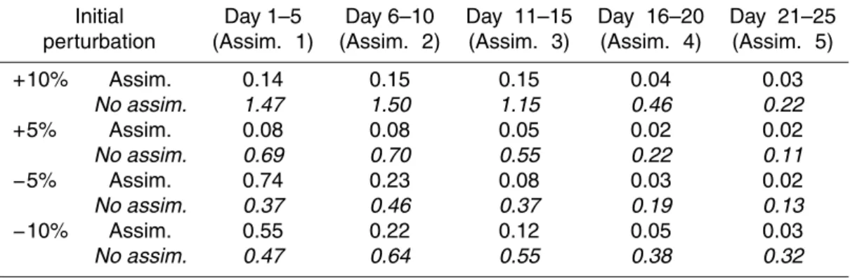
The tests consisted of adding or removing 5% to 10% of the soil water content of all the assimilated basins into the initial state of ISBA soil moisture on 17 February 2006 5

(4 different experiments, Table 1). These initial conditions induced severe floods or droughts, at the beginning of the simulated period, which tended to diminish over time. A reference SIM run was used to generate the synthetic observations.

The results of the 4 assimilation studies are presented in Table 1 and compared to 4 perturbed experiments without any assimilation performed. Table 1 presents the 10

Ratio-rmse (see Appendix B for definition) of simulated SIM streamflows consecutive to the initial perturbation, during the first five assimilation periods. The first experiment (+10% initial state) shows that the assimilation was very effective, reducing the Ratio-rmse to values under 0.15 even for the first assimilation time step, while this score was largely higher than 1 without assimilation for the first assimilation periods. The second 15

experiment (+5% initial state) had the same global behaviour. However, the−5% and −10% experiments did not behave in the same way. The first assimilation time step for these two experiments seemed to be useless, with a Ratio-rmse of the same order as in the corresponding non-assimilated experiment or even higher. In fact, the assimilation “over-corrected” the error. Then, the following assimilations reduced the Ratio-rmse to 20

values lower than 0.1, which was markedly better than the non-assimilated experiment. This “over-correction” (the first assimilation time step led, in fact, to a soil moisture 1 to 2% wetter on average than the reference state) was probably due to the non-respect of the linearity hypothesis: theHmatrix was computed (for the first assimilation process) for dry values of soil moisture (largely below the field capacity value w_{f c}) due to the 25

(16)

HESSD

7, 2413–2453, 2010

G. Thirel et al.

Title Page

Tables Figures

◭ ◮

Back Close

Full Screen / Esc

state, the linear hypothesis was not respected for this first assimilation. However, the system converged rapidly, and it seems important to note that the initial perturbations imposed for these twin experiments were unrealistic and, indeed, huge. For real cases, as described in the following, the increments given by the BLUE are smaller.

5.2 Assimilation of real observations

5

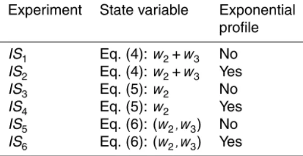
Six experiments are described in this section: the three previously described state vari-ables were used (see Eqs. 4, 5 and 6) and, for each one, two different physics schemes were tested in ISBA (with or without the exponential profile of hydraulic conductivity in the soil). These experiments are summarized in Table 2 with a reference name that is used in all that follows. For theIS1,IS3 andIS5 experiments, the balance between 10

RandBmatrices was chosen by testing a range of possible balances on the shorter 3-month period previously used. Then this was extended to, respectively,IS₂,IS₄and

IS6. The goal of this comparison was to find the best possible set of initial states for the ensemble streamflow forecasts based on SIM. That is why the chosen study pe-riod (from 10 March 2005 to 30 September 2006) corresponded to the pepe-riod for which 15

the comparison of the two ensemble streamflow forecasts chains of M ´et ´eo-France had been performed by Thirel et al. (2008). However, the assimilation was started on 2 January 2005 in order to allow a 2-month spin up of the system.

The assimilation of observations was done daily in order the system to react to bad simulations fast. Therefore, the assimilation window was 1-day long. In order to limit 20

the increments not respecting the validity of the linear hypothesis of the BLUE, the increments were limited to a ±10% range. The validity of this hypothesis will be as-sessed in Sect. 5.4. Moreover, for dry soils (soil moisture lower than 1.1w_{f c}), negative increments were limited to−2% since during observed low flows, if the SIM stream-flow was overestimated during several consecutive days, the BLUE tended to dry the 25

(17)

HESSD

7, 2413–2453, 2010

G. Thirel et al.

Title Page

Tables Figures

◭ ◮

Back Close

Full Screen / Esc

of an aquifer, high anthropization of the basin or difficulties in measurements, which cannot be resolved by adjusting the ISBA soil moisture.

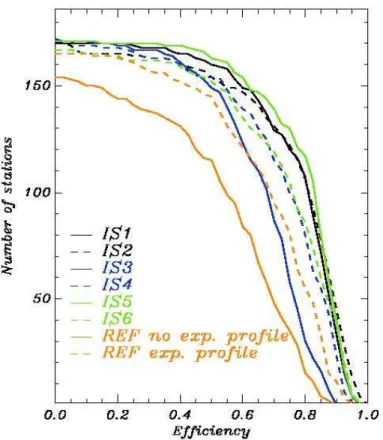
Figure 4 presents the accumulated distribution of efficiency for the 186 assimilated stations, for the 6 experiments plus the two reference simulations of SIM. It shows that the best simulations areIS₁,IS₂andIS₅, and that the improvement in the Nash criterion 5

is significant. For each value of efficiency, the three solid lines are largely higher than the reference solid line. This shows that the experiments with the standard physics of the model (no exponential profile of the hydraulic conductivity) are better than the no-assimilation reference, especially for theIS1 and IS5 experiments. The dashed lines (experiments with the exponential profile of the hydraulic conductivity) are closer to the 10

reference dashed line, because the physics improves the streamflow simulation, but remain above it.

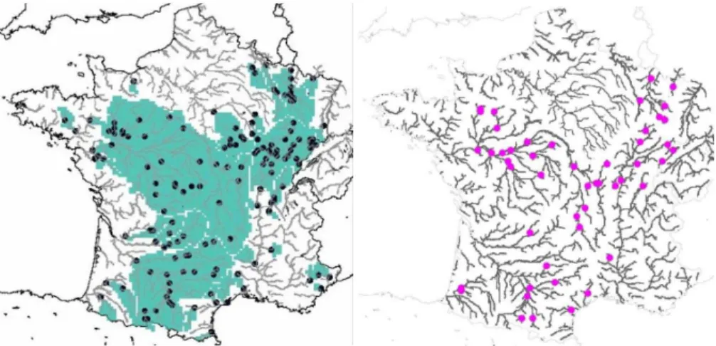
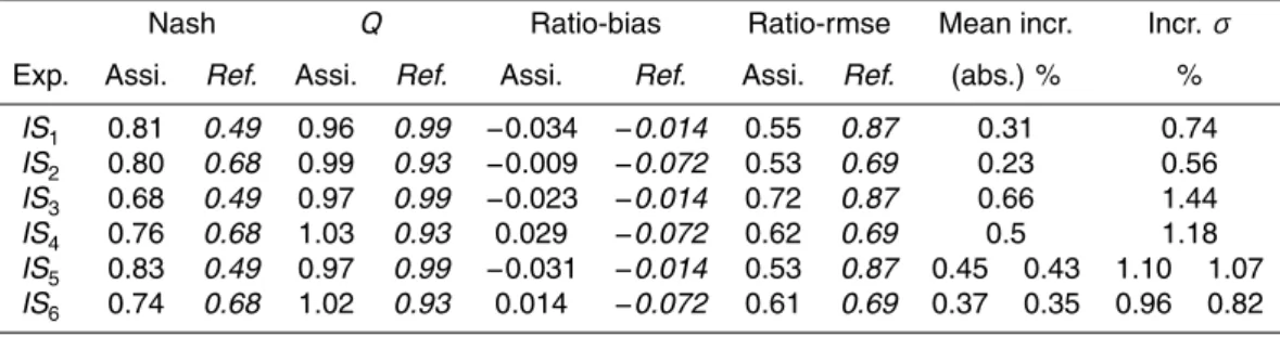
The scores (see Appendix B for definitions) presented in Table 3 are averaged for a selection of 148 stations all over France, out of the 186 available (as shown in Fig. 5 (left)). Stations for which the data assimilation system did not improve the streamflow 15

simulation were excluded here. These stations are located on down-stream parts of the Seine or the Rh ˆone aquifer layers (which are explicitly simulated by SIM). For these basins, the streamflow is mostly affected by the aquifer level rather than by the precipi-tation or the soil water content. Moreover, for some sprecipi-tations, the missing observations were too important so these stations were also excluded.

20

Table 3 shows that, for every experiment, the discharges simulations were improved (better Nash criterion and Ratio-rmse than reference). The assimilation system for ex-periments without the exponential profile of hydraulic conductivity (IS₁,IS₃,IS₅) allowed a greater improvement of the streamflow simulation (when compared to the reference) than theIS2,IS4,IS6 experiments. Since the reference simulation was less accurate 25

(18)

HESSD

7, 2413–2453, 2010

G. Thirel et al.

Title Page

Tables Figures

◭ ◮

Back Close

Full Screen / Esc

The Ratio-rmse, the mean of absolute values of increments, and the spread of the increments were lower for the experiment with the exponential profile of hydraulic con-ductivity (with the same state variable). This means that the assimilation system per-formed better for this experiment (i.e. the Ratio-rmse was reduced), and that smaller changes were imposed by the assimilation system, that is to say the water budget of 5

SIM was less modified. This indicates that the exponential profile of hydraulic conduc-tivity should be chosen, rather than the standard physics of the ISBA scheme, in order to limit the modification of the ISBA prognostic variables by the assimilation. Never-theless, experimentIS5had a better Nash criterion than experimentIS6, for which the only difference was the use of an exponential profile of hydraulic conductivity. This poor 10

performance of theIS₆ experiment can be explained by the fact that the assimilation system acted, in an independent way, on the third soil moisture layer. So it acted di-rectly on the drainage flux to the river, which was a phenomenon having a much longer time-scale than the 1-day assimilation window, with the exponential profile of hydraulic conductivity version of ISBA.

15

It clearly appears that the state variable defined by Eq. (4) (average of the root- and deep-layer soil moistures) gave better results than when defined by Eq. (5) (root layer only). The Nash criterion was the best for these experiments, and the Ratio-rmse, mean increments and spread of increments were lower. The superiority of the Eq. (4) definition over the Eq. (5) one can be explained by the fact that changing only the root-20

layer soil moisture (i.e. Eq. (5) definition) controls the streamflow simulation driven by the runoffalone, not by the drainage. Moreover, a drainage flux of soil water content goes from the root layer to the deep layer, modifying the streamflow simulation, and there is no possibility for the assimilation system to directly act on the deep layer if too much water is added there.

25

With a comparable Nash criterion of about 0.8, the three best experiments wereIS₁

(19)

HESSD

7, 2413–2453, 2010

G. Thirel et al.

Title Page

Tables Figures

◭ ◮

Back Close

Full Screen / Esc

improved with respect to the physics ofIS₅, it can be assumed that the assimilation system contribution should be maintained over longer periods. It is also important to notice that the CPU time cost ofIS5is twice that ofIS1 orIS2. The same conclusions (except for the computational cost) can be drawn betweenIS₁andIS₂, illustrating that

IS2should be preferred toIS1. 5

The best configuration for assimilating the streamflows in SIM appears to be IS2. Moreover, the mean of the absolute values of the increments (0.23%) for this experi-ment is comparable to the value, 0.1%, of the perturbation used to compute the Jaco-bian matrix for the BLUE. This reveals that the assimilation system should respect the linearity hypothesis of the BLUE most of the time. This will be assessed below.

10

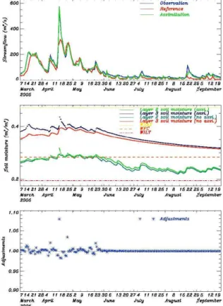
The behaviour of theIS₂assimilation process during a shorter 200-day period is ex-amined in Fig. 6 for streamflows (Fig. 6a), layer 2 and 3 soil moistures (averaged over the sub-basin considered, Fig. 6b), and BLUE increments (Fig. 6c), for the specific case of the River Doubs at Besanc¸on. This period was characterized by a wet period with several flood events, followed by a dryer period. The assimilation was remark-15

ably efficient for the flood events. For the largest flood, the assimilated streamflow was very close to the observation (560 m3s−1) whereas the no-assimilation simulation did not produce values beyond 320 m3s−1. The assimilation system seemed quite sen-sitive and reactive during this period, with mean absolute values of increments being regularly larger than 1% of the soil water content. The soil moisture was wetter with 20

assimilation than without. For the largest flood, the increment was very large (+8%), allowing SIM to immediately simulate a higher streamflow than it would have otherwise. The assimilation performed fewer corrections during the following dryer period. In fact, hardly any increments were produced during this period and the streamflows were lower than the observations, with few improvements when compared to the reference 25

(20)

HESSD

7, 2413–2453, 2010

G. Thirel et al.

Title Page

Tables Figures

◭ ◮

Back Close

Full Screen / Esc

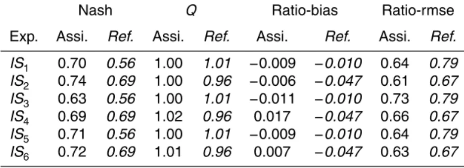
5.3 Validation over independent stations

All the scores previously presented were computed over stations whose discharge ob-servations had been used by the assimilation system. Such a validation is not sufficient to prove that the assimilation works correctly (Talagrand, 2003). For this reason, a se-lection of 49 independent station was used for another validation. These stations, not 5

used by the assimilation system, were located upstream or downstream of the stations used in the assimilation system (see Fig. 5, right). They thus benefited from the better soil moisture of the sub-basins concerned, and from the improved river water content.

Some scores concerning this independent validation are presented in Table 4. Al-though the Nash, Q, Ratio-bias and Ratio-rmse are better for these 49 independent 10

stations than for the 148 stations studied previously when we look at the experiments without assimilation, the scores with assimilation do not show the same behaviour. The 148 stations whose observed discharges were used by the assimilation system have better scores, which is logical. However, it is very interesting that the scores for the 49 independent stations were improved by the assimilation of observed streamflows (ex-15

cept for theIS₄experiment). This overall improvement of the scores of the experiments using the assimilation system shows that this assimilation system is actually effective for improving the SIM river flow simulation.

Here again, the experimentsIS₃andIS₄showed the lowest scores. This was due to the fact that these experiments were already the least efficient for the 148 used stations, 20

and also to the fact that the increments of these two experiments were the highest of the 6 experiments. Thus, with high increments, fluxes were more modified, and the adjustments of the soil moisture did not necessarily lead to discharges simulations fitting the non-used observed discharges. The scores of the four other experiments were very close, with Nash criteria between 0.70 and 0.74, aQratio of 1, a Ratio-bias 25

(21)

HESSD

7, 2413–2453, 2010

G. Thirel et al.

Title Page

Tables Figures

◭ ◮

Back Close

Full Screen / Esc

quality, the use of a better physics scheme, combined with small modifications of the soil moisture, are key ingredients for an improvement of discharges on independent stations. That is why this configuration (IS2, which uses the improved physics and an assimilation method modifying the soil moisture of the deep and root layers jointly) will be chosen to initialize the ensemble streamflow forecasts (Thirel et al., 2010).

5

5.4 Impact of iterations of the BLUE

Using the BLUE to implement a data assimilation system requires using the model in an area of linear behaviour. The linearity is necessary for the BLUE to provide the exact solution to the analysis equation. Of course, with many models, and particularly with hydrological models, linearity is not always respected. It was therefore necessary, 10

in order to verify the relevance of using the BLUE, to investigate this point.

An external loop was implemented on the BLUE, i.e. the BLUE was iterated, until convergence, around the analysis state. In practice, this means that a first iteration of the BLUE was performed (as previously) but then another iteration was performed by computing a new Jacobian matrix around the analysis state given by the first iteration. 15

For this second iteration, the background state modified by this new iteration of the BLUE was once again the one used for the first iteration. Such iterations were per-formed until the decrease of the Ratio-rmse was lower than 0.1 for all the assimilated stations, and a maximum of 10 iterations was fixed. It is obvious that such a process needs at least twice as much CPU time (when the convergence is immediate) and pos-20

sibly 10 times as much CPU time (the maximum number of iterations). Thus, testing of the iterations for this study was limited to theIS2experiment.

The results of the iterations of the BLUE on the scores of the IS2 experiment are presented in Table 5 together with the results of SIM without assimilation but with the improved physics, and the results of the original IS2 experiment. This table shows a 25

(22)

HESSD

7, 2413–2453, 2010

G. Thirel et al.

Title Page

Tables Figures

◭ ◮

Back Close

Full Screen / Esc

the iterations of the BLUE. Finally, the mean of the absolute values of the increments is not modified. All these scores indicate that the contribution of the iterations is very weak, so, because of its prohibitive CPU time cost, its use is far from worthwhile. Moreover, this experiment showed that the linearity of SIM was quite well respected by the past discharge assimilation system, justifying the use of the BLUE for this particular 5

application.

6 Conclusions

The implementation of a streamflow assimilation system in the SIM distributed hydrom-eteorological model has been described in this paper. The performance of this system was assessed for four twin experiments, which showed that the system was efficient 10

in the case of assimilation of synthetic observations. Then the system was assessed for six different configurations over a 569-day period with a set of statistical scores for the assimilation of real observations on 148 dependent stations discharges, and also on 49 independent station discharges. Finally, the respect of the linearity of the model was assessed by studying the contribution of an external loop.

15

The BLUE theory was used for the data assimilation system in the modular coupler PALM. The assimilation system was designed to correct the model soil moisture in or-der to bring the simulated streamflows closer to their true state. Observed streamflows from a total of 186 gauge stations were used. Three choices for the state variable were assessed: considering both layer 2 and layer 3 soil moisture in a single state variable, 20

only considering the layer 2 soil moisture, or considering the soil moisture of the two layers separately. Moreover, the impact of using an improvement in the physics (the use of the exponential profile of hydraulic conductivity) was assessed for each of these choices.

This assimilation system showed results that were very encouraging for the appli-25

(23)

HESSD

7, 2413–2453, 2010

G. Thirel et al.

Title Page

Tables Figures

◭ ◮

Back Close

Full Screen / Esc

observed for each configuration considered, for a selection of 148 assimilated stations. It is important to note that the use of the exponential profile of hydraulic conductivity did not necessarily improve the Nash criterion but, as it reduced the Ratio-rmse, as well as the size of the increments produced by the assimilation system, this physics should be used. For an equivalent streamflow simulation, the less the soil moisture is modified, 5

the better the system performs. Moreover, the benefit of the improved initial state of the assimilation would last longer with this better physics.

The best assimilation (combining high scores and low modification of the model soil moisture) was found for a state variable that was the mean of soil moistures for the two layers with the exponential profile of hydraulic conductivity (IS2experiment). When only 10

the root layer was used, increments were seen to be too large and poor performance was noted. Adjusting the two layers separately could give the best Nash criterion (IS5 experiment) but the overall performance of the assimilation system (bias, rmse, increments) was lower than for theIS₂experiment. TheIS₂ configuration should thus be chosen, in order to combine good performance of the simulation, small soil moisture 15

corrections, and the respect of theQratio.

These conclusions were reinforced by the study of the scores for 49 independent stations. These scores showed the best behaviour of theIS2experiment for the Nash criterion, the Q ratio, the Ratio-bias and the Ratio-rmse. This was due to the better physics used in this configuration and to the low increments imposed by the BLUE. 20

Finally, it was shown that the hypothesis of the linearity ofHwas quite well respected when using the BLUE, as the use of an external loop increased the performance of the system only a little. As the CPU time cost of an external loop is very high, it will not be selected. The improved physics greatly reduced the intensity of the increments, as, it did the respect of the hypothesis of the linearity ofH, showing the interest of using it. 25

(24)

HESSD

7, 2413–2453, 2010

G. Thirel et al.

Title Page

Tables Figures

◭ ◮

Back Close

Full Screen / Esc

the performance of the SIM model. The modularity of the PALM coupler, and the structure of the algorithm as implemented in PALM (perturbed runs of SIM) could also allow the estimation ofK in the BLUE to be easily replaced using Ensemble Kalman Filter, an approach that could handle non-linear effects of the model better (even though these non-linear aspects seemed negligible). Finally, the assimilated basins could be 5

reorganized in order to save CPU time. It could be interesting to subdivide the biggest basins into a smaller number of assimilated sub-basins, thereby reducing the number of perturbed runs of SIM needed to compute the Jacobian matrix.

This study has demonstrated the potential of using a past discharge assimilation sys-tem in order to improve the SIM streamflow simulations and then to provide good quality 10

initial states for ensemble prediction systems. The impact of the IS₂ initial states on the scores of two Ensemble Streamflow Prediction Systems of M ´et ´eo-France (PEARP – and ECMWF-based SIM hydrological forecasts) will be examined in a forthcoming study (Thirel et al., 2010).

Acknowledgements. The authors would like to thank Bertrand Bouriquet (CERFACS) for the

15

assistance he gave to launch the project on its early stages. We are also grateful to Thierry Morel and Anthony Th évenin (CERFACS) for their time spent on technical support of the PALM software, including a special version available for this work on the M ét éo-France NEC super-computer platform, and for their debugging assistance.

We would like to thank Jo ël Noilhan (CNRM-GAME, M ét éo-France, CNRS) who suggested

20

implementing such an assimilation on this distributed hydrometeorological model and using PALM. Discharge observations were provided by the French Hydro database (Minist ère de l’ Écologie, de l’ Énergie, du D éveloppement durable et de la Mer, Direction de l’Eau, http://www. eaufrance.fr), which gathers data from many producers.

(25)

HESSD

7, 2413–2453, 2010

G. Thirel et al.

Title Page

Tables Figures

◭ ◮

Back Close

Full Screen / Esc

Interactive Discussion The publication of this article is financed by CNRS-INSU.

Appendix A

Filling of the Jacobian matrix for a simple main basin

A simple, theoretical example is given here to explain how theHmatrix was computed. 5

Figure 3 represents a schematic river network, where three stations are assimilated. Two upstream sub-basins (subscripts 2 and 3), independent of each other, flow into a larger down-stream sub-basin (subscript 1). xstands for the soil moisture as the state variable, andystands for the streamflow as the observation.

With these three assimilated stations, the Jacobian matrix is a 3×3 matrix (for a 10

“tree”):

H=



  

∆y₁

∆x₁

∆y₁

∆x₂

∆y₁

∆x₃ 0 ∆y2

∆x₂ 0 0 0 ∆y3

∆x₃



  

(A1)

Three perturbed runs of SIM (in addition to a reference run) had to be processed to estimateHcompletely. For the first one, only basin 1 soil moisture was perturbed, with no change to the soil moisture of sub-basins 2 and 3. With this run, the response of 15

station 1 streamflow (y₁) to a perturbation of the soil moisture of sub-basin 1 (x₁) was deduced, and so H1,1 was known (the state variable element corresponding to sub-basin 1 excludes the soil moisture of sub-sub-basins 2 and 3, so its change has no effect on streamflows 2 and 3 (i.e. H_2,1 and H_3,1were null)). Then, when x₂ was perturbed, the response of y2 (H2,2) and y1 (H1,2) were simultaneously deduced. And finally, a 20

(26)

HESSD

7, 2413–2453, 2010

G. Thirel et al.

Title Page

Tables Figures

◭ ◮

Back Close

Full Screen / Esc

For the assimilation of the 186 stations, 34 perturbed runs of SIM were needed (plus 1 non perturbed run), because this is the number of perturbations to be imposed to compute the Jacobian elements of the largest basin (the biggest basin, the Loire basin, has 34 stations). Other independent basins can be treated during the determination of the part of the Jacobian matrix dedicated to the Loire basin.

5

Appendix B

Statistical scores

Four hydrological statistical scores were used for this study: the Ratio-root mean square error (Ratio-rmse), the Ratio-bias, the discharge ratioQ, and the Nash crite-10

rion (or efficiency).

The Ratio-root mean square error (Ratio-rmse) is defined as:

Ratio−rmse= 1 Qobs

v u u u t

T

P

t=1

(Qt_obs−Qt_sim)2

T (B1)

withT the total number of days of the period studied,Qt_obsthe observed discharges (for dayt), Qobs the mean of the observed discharges during the study period, and Q

t sim 15

the simulated discharges (for dayt). The Ratio-bias is computed as:

Ratio−bias=

T

P

t=1

(Qt_obs−Qt_sim)

T·Qobs

(27)

HESSD

7, 2413–2453, 2010

G. Thirel et al.

Title Page

Tables Figures

◭ ◮

Back Close

Full Screen / Esc

The discharge ratio (Q) is the ratio between the mean simulated discharges and the mean observed discharges:

Q=Qsim Qobs

(B3)

And finally, the Nash criterion (E, efficiency) is:

E=1− T

P

t=1

(Qt_obs−Qt_sim)2

T

P

t=1

(Qt_obs−Qobs)2

(B4) 5

The Nash criterion is a score of between−∞and 1, and it is often considered that a score higher than 0.7 characterizes a very good simulation of the discharges. Further-more, this score, by its definition, is very sensitive to flood errors.

References

Aubert, D., Loumagne, C., and Oudin, L.: Sequential Assimilation of Soil Moisture and

Stream-10

flow Data in a Conceptual Rainfall-RunoffModel, J. Hydrol., 280, 145–161, 2003. 2416 Boone, A., Calvet, J. C., and Noilhan, J.: Inclusion of a Third Soil Layer in a Land Surface

Scheme Using the Force-Restore Method, J. Appl. Meteorol., 38, 1611–1630, 1999. 2417, 2422

Boone, A. and Etchevers, P.: An Intercomparison of Three Snow Schemes of Varying

Com-15

plexity Coupled to the Same Land Surface Model: Local-Scale Evaluation at an Alpine Site, J. Hydrometeorol., 2, 374–394, 2001. 2417

Bouttier, F. and Courtier, P.: Data assimilation concepts and methods, ECMWF Lecture notes, 58 pp., 1999. 2420

Brasseur, P., Bahurel, P., Bertino, L., et al.: Data assimilation in operational ocean forecasting

20

(28)

HESSD

7, 2413–2453, 2010

G. Thirel et al.

Title Page

Tables Figures

◭ ◮

Back Close

Full Screen / Esc

Interactive Discussion Buis, S., Piacentini, A., and D ´eclat, D.: PALM: A Computational framework for assembling high

performance computing applications, Concurrency and computation: practice and experi-ence, 18(2), 247–262, 2006. 2419

Buizza, R., Bildot, J.-R., Wedi, N., Fuentes, M., Hamrud, M., Holt, G., and Vitart, F., The new ECMWF VAREPS (Variable Resolution Ensemble Prediction System), Q. J. Roy. Meteor.

5

Soc., 133, 681–695, 2007. 2415

Chessa, P. A. and Lalaurette, F.: Verification of ECMWF Ensemble Prediction System forecasts: A study of large-scale patterns, Weather Forecast., 16, 611–619, 2001. 2415

Clark, M. P., Rupp, D. E., Woods, R. A., Zheng, X., Ibbitt, R. P., Slater, A. G., Schmidt, J., and Uddstrom, M. J.: Hydrological data assimilation with the ensemble Kalman filter: Use

10

of streamflow observations to update states in a distributed hydrological model, Adv. Water Resour., 31, 10, 1309–1324, 2008. 2416

Durand, Y., Brun, E., Merindol, L., Guyomarc’h, G., Lesaffre, B., and Martin, E.: A meteoro-logical estimation of relevant parameters for snow schemes used with atmospheric models, Ann. Glaciol., 18, 65–71, 1993. 2417

15

Etchevers, P., Golaz, C. and Habets, F.: Simulation of the water budget and the river flows of the Rh ˆone basin from 1981 to 1994, J. Hydrol., 244, 60–85, 2001. 2418

Fouilloux, A. and Piacentini, A., The PALM Project: MPMD Paradigm for an Oceanic Data Assimilation Software, Lecture Notes In Computer Science, 1685, 1423–1430, 1999. 2419 Habets, F., Etchevers, P., Golaz, C., Leblois, E., Ledoux, E., Martin, E., Noilhan, J., and Ottl ´e,

20

C.: Simulation of the water budget and the river flows of the Rh ˆone basin, J. Geophys. Res., 104, 31145–31172, 1999a. 2417

Habets, F., Noilhan, J., Golaz, C., Goutorbe, J. P., Lacarr `ere, P., Leblois, E., Ledoux, E., Martin, E., Ottl ´e, C., and Vidal-Madjar, D.: The ISBA surface scheme in a macroscale hydrological model, applied to the HAPEX-MOBILHY area: Part 2 simulation of streamflows and annual

25

water budget, J. Hydrol., 217, 97–118, 1999b. 2417

Habets, F., Boone, A., Champeau, J. L., Etchevers, P., Leblois, E., Ledoux, E., Lemoigne, P., Martin, E., Morel, S., Noilhan, J., Quintana Segu´ı, P., Rousset-Regimbeau, F., and Vien-not, P.: The SAFRAN-ISBA-MODCOU hydrometeorological model applied over France, J. Geophys. Res., 113, D06113, doi:10.1029/2007JD008548, 2008. 2418

30

Komma, J., Bl ¨oschl, G., and Reszler, C.: Soil moisture updating by Ensemble Kalman Filtering in real-time flood forecasting, J. Hydrol., 357, 228 242, 2008. 2416

(29)

HESSD

7, 2413–2453, 2010

G. Thirel et al.

Title Page

Tables Figures

◭ ◮

Back Close

Full Screen / Esc

Interactive Discussion the PALM flow charting approach, Q. J. Roy. Meteor. Soc., 127, 189–207, 2001. 2419

Ledoux, E., Girard, G., de Marsilly, G. and Deschenes, J.: Spatially distributed modeling: Con-ceptual approach, coupling surface water and groundwater, Unsaturated Flow Hydrologic Modeling, edited by: Morel-Seytoux, H. J., Theory and Practice, NATO ASI Series C, Kluwer, 275, 435–454, 1989. 2418

5

Morel, S.: Mod élisation à l’ échelle r égionale des bilans énerg étique et hydrique de surface et des d ébits; application au bassin Adour-Garonne (Modeling at a regional scale of surface and streamflows energetic and hydric balance sheet), Ph.D. Thesis, Universit é Paul Sabatier, Toulouse, France, 280 pp., 2003. 2418

Noilhan, J. and Mahfouf, J.-F.: The ISBA land surface parameterization scheme, Global Planet.

10

Change, 13, 145–159, 1996. 2417

Noilhan, J. and Planton, S., A simple parametrization of land surface processes for meteoro-logical models, Mon. Weather Rev., 117, 536–549, 1989. 2417

Nicolau, J.: Short-range ensemble forecasting at M ´et ´eo-France - A preliminary study, Proc. Tech. Conf. on Data Processing and Forecasting Systems, Cairns, QLD, Australia,

15

WMO/Commission on Basic Systems, available at: http://www.wmo.int/pages/prog/www/ DPS/TC-DPFS-2002/Papers-Posters/Topic1-Nicolau.pdf, 2002.

Quintana, C., Segu´ı, P., Le Moigne, P., Durand, Y., Martin, E., Habets, F., Baillon, M., Canellas, Franchisteguy, L., and Morel, S.: Analysis of near surface atmospheric variables: Validation of the SAFRAN analysis over France, J. Appl. Meteorol. Clim., 47, 92–107, 2008. 2417,

20

2424

Quintana Segu´ı, P., Martin, E., Habets, F., and Noilhan, J.: Improvement, calibration and vali-dation of a distributed hydrological model over France, Hydrol. Earth Syst. Sci., 13, 163–181, 2009,

http://www.hydrol-earth-syst-sci.net/13/163/2009/. 2417, 2418

25

Ramos, M.-H., Bartholomes, J., and del Pozo, J. T.: Development of decision support products based on ensemble forecasts in the European Flood Alert System, Atmos. Sci. Lett., 8, 113– 119, 2007. 2415

Reichle, R. H., Walker, J. P., Koster, R. D., and Houser, P. R.: Extended versus Ensemble Kalman Filtering for Land Data Assimilation, J. Hydrometeorol., 3(6), 728–740, 2002. 2415

30

(30)

HESSD

7, 2413–2453, 2010

G. Thirel et al.

Title Page

Tables Figures

◭ ◮

Back Close

Full Screen / Esc

Interactive Discussion Rousset-Regimbeau, F., Habets, F., Martin, E., and Noilhan, J.: Ensemble streamflow forecasts

over France, ECMWF Newsletter No. 111, Spring, 2007. 2415, 2418

R ¨udiger, C.: Streamflow Data Assimilation for Soil Moisture Prediction, Ph.D. thesis, Dept. of Civil & Environmental Engineering, The University of Melbourne, 414 pp., 2006. 2415 Schaake, J., Franz, K., Bradley, A., and Buizza, R.: The Hydrologic Ensemble Prediction

EX-5

periment (HEPEX), Hydrol. Earth Syst. Sci. Discuss., 3, 3321–3332, 2006, http://www.hydrol-earth-syst-sci-discuss.net/3/3321/2006/. 2415

Seo, D-J., Cajina, L., Corby, R., and Howieson, T.: Automatic state updating for operational streamflow forecasting via variational data assimilation, J. Hydrol., doi: 10.1016/j.jhydrol.2009.01.019, 2009. 2416

10

Talagrand, O.: Objective Validation and Evaluation of Data Assimilation, Proceedings of Semi-nar on Recent developments in data assimilation for atmosphere and ocean, SemiSemi-nar Series on Recent developments in atmospheric and ocean data assimilation, 287–299, ECMWF, Shinfield Park, Reading, 8–12 September, 2003. 2432

Thirel, G., Rousset-Regimbeau, R., Martin, E., and Habets, F.: On the Impact of Short-Range

15

Meteorological Forecasts for Ensemble Streamflow Predictions, J. Hydrometeorol., 9, 1301– 1317, 2008. 2415, 2418, 2428

Thirel, G., Martin, E., Mahfouf, J.-F., Massart, S., Ricci, S., Regimbeau, F., and Habets, F.: A past discharges assimilation system for ensemble streamflow forecasts over France, Part 2: Impact on the ensemble streamflow forecasts, Hydrol. Earth Syst. Sci. Discuss., 7,

2455-20

2497, 2010. 2433, 2436

Zaitchik, B. F., Rodell, M., and Reichle, R. H.: Assimilation of GRACE Terrestrial Water Storage Data into a Land Surface Model: Results for the Mississippi River Basin, J. Hydrometeorol., 9, 535–548, 2008.

(31)