The Good, The Fast And The Better Pedestrian Detector

(1)

THE GOOD, THE FAST AND THE BETTER

(2)

(3)

ARTUR JORDÃO LIMA CORREIA.

THE GOOD, THE FAST AND THE BETTER

PEDESTRIAN DETECTOR

Dissertação apresentada ao Programa de Pós-Graduação em Ciência da Computação do Instituto de Ciências Exatas da Univer-sidade Federal de Minas Gerais - Departa-mento de Ciência da Computação. como requisito parcial para a obtenção do grau de Mestre em Ciência da Computação.

Orientador: William Robson Schwartz

Belo Horizonte

(4)

(5)

ARTUR JORDÃO LIMA CORREIA.

THE GOOD, THE FAST AND THE BETTER

PEDESTRIAN DETECTOR

Dissertation presented to the Graduate Program in Ciência da Computação of the Universidade Federal de Minas Gerais - De-partamento de Ciência da Computação. in partial fulfillment of the requirements for the degree of Master in Ciência da Com-putação.

Advisor: William Robson Schwartz

Belo Horizonte

(6)

c

Artur Jordão Lima Correia.

C824g The Good, the Fast and the Better pedestrian detector / Artur Jordão Lima Correia.. — Belo Horizonte, 2016

xx, 51 f. : il. ; 29cm

Dissertação (mestrado) — Universidade Federal de Minas Gerais - Departamento de Ciência da

Computação.

Orientador: William Robson Schwartz

1. Computação - Teses. 2. Visão por computador -Teses. 3. Teoria da estimativa - Teses. 4. Detecção de pedestres. I.Orientador. II Título.

(7)

(8)

(9)

Acknowledgments

I am eternally thankful for all support that my parents gave me, allowing me to focus on research and studies.

I would like to thank deeply professor William Robson Schwartz for the outstand-ing orientation on my graduate study.

A special thanks to my friends: Bruno Salomão, Felipe Casanova, Fernando Plantier, Caio Russi, Arthur Santos, Renan Ferreira (Xisto), Pedro Machado, An-derson Gohara, Guilherme Potje, Thais Lima, Renata Boin and Ana Flávia, for the sincere friendship.

Also, I thank my colleagues in Federal University of Minas Gerais: Luis Pedraza, André Costa, Leandro Augusto, Thiago Rodrigues, Gabriel Gonçavels, Clebson Car-doso, Ricardo Kloss, Jessica Senna, Victor Melo, Antonio Nazaré, Marco Tulio, Rensso Mora, Cássio Elias, Rafael Vareto, Carlos Caetano, Ramon Pessoa, Raphael Prates, César Augusto.

I would like to thank the Brazilian National Research Council – CNPq (Grant #477457/2013-4), the Minas Gerais Research Foundation – FAPEMIG (Grants APQ-00567-14 and PPM-00025-15) and the Coordination for the Improvement of Higher Education Personnel – CAPES (DeepEyes Project).

(10)

(11)

Resumo

Detecção de pedestres é um bem conhecido problema em Visão Computacional, prin-cipalmente por causa de sua direta aplicação em vigilância, segurança de trânsito e robótica. Na última década, vários esforços têm sido realizados para melhorar a de-tecção em termos de acurácia, velocidade e aprimoramento de features. Neste tra-balho, nós propomos e analisamos técnicas focando sobre estes pontos. Primeiro, nós desenvolvemos uma acurada random forest oblíqua (oRF) associada comPartial Least Squares (PLS). O método utiliza o PLS para encontrar uma superfície de decisão, em cada nó de uma árvore de decisão. Para mensurar as vantagens providas pelo PLS so-bre o oRF, nós comparamos o método proposto com a random forest oblíqua baseada em SVM. Segundo, nós avaliamos e comparamos abordagens de filtragem para reduzir o espaço de busca e manter somente regiões de potencial interesse para serem apresen-tadas para os detectores, acelerando o processo de detecção. Resultados experimentais demonstram que os filtros avaliados são capazes de descartar um grande número de janelas de detecção sem comprometer a acurácia. Finalmente, nós propomos uma nova abordagem para extrair poderosasfeatures em relação à cena. O método combina resul-tados de distintos detectores de pedestres reforçando as hipóteses humanas, enquanto que suprime um significante número de falsos positivos devido á ausência de consenso espacial quando múltiplos detectores são considerados. A abordagem proposta, referida como Spatial Consensus (SC), supera os resultados de todos os métodos de detecção de pedestres previamente publicados.

(12)

(13)

Abstract

Pedestrian detection is a well-known problem in Computer Vision, mostly because of its direct applications in surveillance, transit safety and robotics. In the past decade, several efforts have been performed to improve the detection in terms of accuracy, speed and feature enhancement. In this work, we propose and analyze techniques focusing on these points. First, we develop an accurate oblique random forest (oRF) associated with Partial Least Squares (PLS). The method utilizes the PLS to find a decision surface, at each node of a decision tree, that better splits the samples presented to it, based on some purity criterion. To measure the advantages provided by PLS on the oRF, we compare the proposed method with the oRF based on SVM. Second, we evaluate and compare filtering approaches to reduce the search space and keep only potential regions of interest to be presented to detectors, speeding up the detection process. Experimental results demonstrate that the evaluated filters are able to discard a large number of detection windows without compromising the accuracy. Finally, we propose a novel approach to extract powerful features regarding the scene. The method combines results of distinct pedestrian detectors by reinforcing the human hypothesis, whereas suppressing a significant number of false positives due to the lack of spatial consensus when multiple detectors are considered. Our proposed approach, referred to as Spatial Consensus (SC), outperforms all previously published state-of-the-art pedestrian detection methods.

Keywords: Random Forest, Oblique Decision Tree, Partial Least Squares, Filtering Approaches, High-Level Information, Fusion of Detectors, Pedestrian Detection.

(14)

(15)

List of Figures

1.1 Detection pipeline used to find people in images. . . 2

3.1 Pipeline detection and its respective section. . . 13 3.2 Decision tree split types (the bars represent the information gain). . . 15 3.3 Translucent areas demonstrate regions eliminated by filtering stage for

dif-ferent filtering approaches. . . 18 3.4 Different regions of the image (detection windows) captured by sliding

win-dows approach and their respective magnitude images where M is the av-erage gradient magnitude computed from each region using Equation 3.10. 19 3.5 Sliding window approach on saliency map. . . 21 3.6 Detection results and their respective heat map. . . 22 3.7 Different aspects between our proposed Spatial Consensus algorithm and

the weighted-NMS [Jiang and Ma, 2015]. . . 25

4.1 Image examples from the datasets used in this work. . . 28 4.2 Log-average miss rate achieved in each bootstrapping iteration using

oRF-PLS and oRF-SVM, respectively, on validation set. . . 30 4.3 Log-average miss-rate (in percentage points) on the validation set as a

func-tion of the number of trees. . . 31 4.4 Comparison of our oRF-PLS approach with the state-of-the-art. . . 32 4.5 Tradeoff between scale factor and number of windows generated for a640×

480 image. . . 33 4.6 Threshold approaches analyzed to be used as rejection criteria in the

saliency map. . . 34 4.7 Relationship between rejection percentage and recall achieved by filters

(as-suming that an ideal detector was employed after the filtering stage). . . . 35 4.8 Number of false positives as a function of the number of detectors added

and the thresholdσ (results on INRIA Person dataset). . . 39

(16)

4.9 Comparison between our proposed method with the baseline in terms of improvement and depreciation (according todetroot) of the log-average miss rate. . . 40 4.10 Comparison of our proposed approach with the state-of-the-art. . . 44

(17)

List of Tables

2.1 Overview of state-of-the-art detectors on INRIA person dataset, sorted by

log-average miss-rate. . . 11

4.1 Miss rate obtained at100 _{FPPI with different scale factors. . . .} ₃₄

4.2 Miss rate at 100 _{FPPI applying the filtering stage on the detectors. . . . .} ₃₆

4.3 INRIA Person Detectors Accumulation. . . 37

4.4 ETH Detectors Accumulation. . . 37

4.5 Caltech Detectors Accumulation. . . 37

(18)

(19)

Chapter 1 Introduction

Since the past decade, pedestrian detection has been an active research topic in Com-puter Vision, mostly because of its direct applications in surveillance, transit safety and robotics [Benenson et al., 2014]. This task faces many challenges, such as variance in clothing styles and appearance, distinct illumination conditions, frequent occlusion among pedestrians and high computational cost.

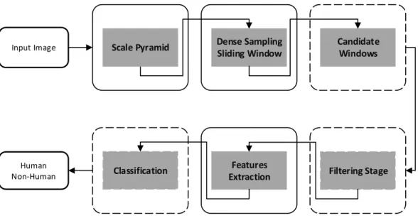
Figure 1.1 introduces the steps employed by traditional approaches to detect pedestrians in an image. First, the image is downsampled by a scale factor generating a set of new images, this procedure is named scale pyramid. Then, a window slides on each image of the pyramid yielding several candidate windows. Once the candidates have been generated, they might be presented to an optional filtering stage, employed to remove a large number of windows quickly. Finally, for each candidate window, features are extracted and presented to a classifier that assigns a score, which will be considered as the likelihood of having a pedestrian located at the particular location in the image. Different challenges are found throughout this pipeline and this work addresses some of them. More specifically, we tackle these challenges by acting on three main points: classification, candidate rejection, and fusion of detectors.

According to Benenson et al. [2014], the most promising pedestrian detection methods are based on deep learning and random forest. Despite accurate, deep learning approaches (commonly convolutional neural networks) require a powerful hardware architecture and considerable amount of samples to learn a model. Moreover, the best results associated to such approaches are comparable with simpler methods [Dollár et al., 2012; Benenson et al., 2014]. On the other hand, random forest approaches are able to run on simple CPU architecture and can be learned with fewer samples. The increasing number of studies based on this classifier is due several advantages that this approach presents including low computational cost to test, probabilistic output and

(22)

2 Chapter 1. Introduction

Input Image

Human Non-Human

Scale Pyramid Dense Sampling Sliding Window

Classification Features Extraction

Candidate Windows

Filtering Stage

Figure 1.1. Detection pipeline used to find people in images.

it naturally treats problems with more than two classes [Criminisi and Shotton, 2013].

Following the definition of Breiman [2001], a random forest is a set of decision trees, in which the response is a combination of all tree responses at the forest. We can classify a random forest according to the type of the decision tree that it is composed: orthogonal or oblique. In the former type, each tree node creates a boundary decision axis-aligned, i.e, it divides the data selecting an individual feature at a time. The latter type separates the data by oriented hyperplanes, providing better data separation and shallower trees [Menze et al., 2011]. Inspired by these features, in the first part of this work, we propose a novel oblique random forest (oRF) associated with Partial Least Squares (PLS) [Jordao and Schwartz, 2016], which is a popular technique to dimensionality reduction and regression [Schwartz et al., 2009, 2011; de Melo et al., 2014].

(23)

3

2010; Benenson et al., 2012a]; and (iv) filtering regions of interest [Silva et al., 2012; de Melo et al., 2014]. Among the aforementioned approaches, filtering regions of inter-est is a simple and effective way of speeding up the detection. Filtering approaches are performed before of the feature extraction and classification stage, and focus on reduc-ing the amount of data that has to be processed, allowreduc-ing the consideration of fewer samples (detection windows), reducing the computational cost. Such approaches are based on two prior knowledges: (1) only a subset of all detection windows contains the target object (the distribution between pedestrian and non-pedestrian is largely unbal-anced) and (2) several detection windows cover the same object at the scene [de Melo et al., 2013; Silva et al., 2012; de Melo et al., 2014].

Although filtering approaches are effective, it is unclear which filters are more ap-propriate according to the detector employed since there is not a study evaluating this relationship. Even though similar studies have been performed in previous works [Dol-lár et al., 2009, 2014], where several techniques to improve the detection rate were evaluated, to the best of our knowledge, there is not a comparison among filters in terms of efficiency and robustness, i.e., the ability of rejecting candidate windows while preserving a high detection rate. This motivated the second part of our work, where we evaluate and compare filtering approaches to both reduce the search space and keep only potential regions of interest to be presented to detectors [Jordao et al., 2015].

While numerous classification methods and optimization approaches have been investigated, the majority of efforts in pedestrian detection in the last years can be attributed to the improvement in features alone and evidences suggest that this trend will continue [Dollár et al., 2012; Benenson et al., 2014]. In addition, several works show that the combination of features creates a more powerful descriptor which improves the detection [Schwartz et al., 2009; Dollár et al., 2009; Marín et al., 2013]. Despite the combination of features provide a better discrimination, pedestrian detection is still dealing with some problems. The existence of false positives, such as lampposts, tree and plates, which are very similar to the human body, is a difficult problem to solve. To address this problem, previous works employed high level information regarding the scene to refine the detections [Schwartz et al., 2011; Li et al., 2010; Benenson et al., 2014; Jiang and Ma, 2015].

(24)

the confidence. However, when the windows do not overlap, their method keeps both, which might increase the number of false positives (details in Section 3.3). Aiming at tackling such limitation, in the third part of this work, we propose a novel late fusion method called Spatial Consensus (SC) to combine multiple detectors [Jordao et al., 2016].

According to the experimental results, the proposed oblique random forest based on PLS (oRF-PLS) achieves comparable results when compared with traditional meth-ods based on HOG features. Besides, we demonstrate that a smaller forest is produced when compare to the oblique random forest based on SVM (oRF-SVM). In the exper-iments considering the filtering approaches, we demonstrate that the evaluated filters are able to discard a large number of windows without compromising the detection accuracy. Finally, regarding the spatial consensus algorithm, experiments showed that it outperforms the state-of-the-art, achieving the best results in all evaluated datasets.

1.1 Motivation

An important application involving the pedestrian detection is to improve the efficient of the work of a human operator. For instance, large surveillance centers demand which a single operator observes several cameras at the same time to find suspicious activities. However, studies show that in a short time the concentration is lost since this activity is routine and monotonous [Smith, 2004]. To avoid that, pedestrian detection algorithms might be employed to attract the operator’s attention to a determined camera (or another surveillance device) and relevant regions of the scene, improving the efficient of the work. Another target in detect people in images is directed to automatic systems applications, e.g, driving assistance and robotics. In these applications, the pedestrian detection assists on the decision-making, focusing on avoiding damage to the humans and the environment. The issues listed above require a robust and accurate pedestrian detection, these requirements motivated us to propose and study a series of techniques focused on improvement of pedestrian detection.

Our first center of attention regards the classification stage associated with oblique random forest. Such class of random forest is commonly generated using the SVM as oriented hyperplane (details in Section 3.1.2). This inspired the first part of our work, where we demonstrate experimentally that the PLS provide a more accurate oblique random forest than SVM [Jordao and Schwartz, 2016].

(25)

1.2. Objectives ₅

the second part of our work, in which we consider several optimization approaches to keep only regions of the scene where there is the object of interest [Jordao et al., 2015]. Therewith, a smaller number of candidate windows are propagated to the classifica-tion stage to allow a faster pedestrian detecclassifica-tion without compromising the detecclassifica-tion accuracy.

The promising results using high level information regarding the scene to refine detections [Schwartz et al., 2011; Li et al., 2010; Benenson et al., 2014; Jiang and Ma, 2015] motivated the third part of our work, where we propose a novel late fusion method to combine the responses coming from multi-detectors [Jordao et al., 2016].

1.2 Objectives

This work targets the problem of finding people in images through use distinct ways in different stages of the detection (see Figure 1.1). We can divide the objectives into three main parts, as follows. First, we intend to demonstrate the advantage of the PLS as alternative to build the oblique random forest. To this end, we employed another accurate classifier to produce the oblique random forest, the SVM. Second, we intend to evaluate the behavior of the filters approaches when employed on different detectors. To this analysis, we collect the main filters used in the pedestrian detection context. Third, we demonstrate that information coming from multiple detectors can improve the detection, increasing the confidence of true positives. To evidence that, we propose a novel late fusion method that enable such combination and we showed experimentally that our method is a more suitable choice to fuse detectors when compared with the weighted-NMS (a recent approach to combine detectors) [Jiang and Ma, 2015].

1.3 Contributions

Our first contribution is a novel alternative to generate the oRF to providing a smaller forest when compared with the traditional oRF-SVM [Jordao and Schwartz, 2016]. Our second contribution is a detailed study of a series of filtering approaches that provide a lower computational cost to the detection [Jordao et al., 2015]. Finally, our last contribution is a novel late fusion approach that enable to combine multi-detectors improving the detection [Jordao et al., 2016].

The publications achieved with this work are listed as follows.

(26)

Computacional (WVC), pages 1-8.

2. Jordao, A., de Souza, J. S., and Schwartz, W. R. A Late Fusion Approach to Combine Multiple Pedestrian Detectors. In IEEE Transactions on Image Pro-cessing (ICPR).

3. Jordao, A. and Schwartz, W. R. Oblique random forest based on partial least squares applied to pedestrian detection. In IEEE International Conference on Image Processing (ICIP).

1.4 Work Organization

(27)

Chapter 2 Related Work

In this chapter, we present an overview regarding the main approaches employed in the pedestrian detection context. Initially, we discuss the main feature descriptors employed to describe human samples and background samples. Then, we review ap-proaches used to reduce the computational cost to enable faster detection. Finally, we demonstrate techniques applied after the detection stage to improve the detection.

The detector based on the Histogram of Oriented Gradients (HOG) features pro-posed by Dalal and Triggs [2005] enabled impressive advances in several object recog-nition tasks, mainly on the pedestrian detection problem. On their initial work, Dalal and Triggs proposed to divide the detection windows in blocks of 16×16 pixels with shift of 8×8 pixels between blocks to compute the HOG features. Zhu et al. [2006] then showed that extracting HOG with different block sizes and strides, could lead to a more discriminative descriptor. Following the work of Zhu et al. [2006], Schwartz et al. [2009] employed similar block configurations to extract HOG features and with the addition of extra information provided by co-occurrence and color frequency fea-tures, the detector proposed by Schwartz et al. [2009] was able to reducing considerably the false positives. However, these features when combined yield a high dimensional feature space, rendering many traditional machine learning techniques intractable. To address that, the authors employed the partial least squares (PLS) to reduce the high dimensional feature space onto a low dimensional latent space before projecting itself to Quadratic Discriminant Analysis (QDA) performs the classification.

Similarly to Schwartz et al. [2009], several works showed that the combination of features creates a more powerful descriptor that improves the detection [Dollár et al., 2009; Marín et al., 2013]. A classical example of feature combination widely-used is the HOG with local binary patter (LBP), HOG+LBP [Wang et al., 2009]. This merge has been shown efficient since HOG describes the shape information while the LBP capture

(28)

8 Chapter 2. Related Work

the texture of the object, both important clues to find people in images. Marín et al. [2013] employed this combination to describe human regions with high discriminative power, achieving a detector robust to partial occlusions. In contrast to Marín et al. [2013], Costea and Nedevschi [2014] combined HOG+LBP and LUV color channels in a high level visual words named word channels allowing detection of pedestrians of different sizes on single scale image, which considerably reduces the computational cost.

Another feature combination that present good results to object detection are the Integral Channel Features (ICF) [Dollár et al., 2009]. Proposed by Dollár et al. [2009], the ICF features consists on ten channels of features: HOG (6 channels), LUV color channels (3 channels) and normalized gradient magnitude (1 channel). All these feature channels are extracted using the Integral Image trick, which render the feature extraction process extremely fast [Gerónimo and López, 2014]. Due to its simplicity and low computational cost, ICF features are the most predominant features explored in pedestrian detection, as illustrates Table 2.1. That table lists the main state-of-the-art pedestrian detectors on INRIA person dataset and synthesizes the essential features of each detector instead of discussing each one individually. An important aspect to be pointed out is that the Adaboost classifier is usually a preferential choice since its classification is very fast, mainly when combined with ICF features.

Adaboost classifier consists on an ensemble of classifiers that are combined to make prediction once test samples are presented. Generally, weak classifiers as decision stumps and orthogonal decision forest are chosen to compose the ensemble. However, some works [Criminisi and Shotton, 2013; Marín et al., 2013] have shown promising results when using strong classifiers (for instance SVM) on the ensemble. Inspired by these works [Criminisi and Shotton, 2013; Marín et al., 2013], we analyze, in the first part of our work (Section 3.1), the performance of the PLS as alternative to the SVM to creating ensemble members, focusing on oblique decision trees.

An alternative to enable a faster pedestrian detection independently of features and the classifier utilized are two main class: parallelization and use of GPUs [Masaki et al., 2010; Benenson et al., 2012b], and filtering regions of interest [Hou and Zhang, 2007; Silva et al., 2012; de Melo et al., 2014]. The latter is a simple but effective manner of speeding up the detection. In the next paragraph, we review the main filtering approaches applied to object recognition tasks.

(29)

9

To find objects in the imageI, the authors applied a threshold, τ, on the saliency map S(I). This threshold was empirically estimated as τ = 3E(S(I)), where E represents the average of intensity in the saliency map. Silva et al. [2012] proposed an extension of Hou and Zhang [2007] to pedestrian detection, where a saliency map was build for multiple scales. Different from of Hou and Zhang [2007], Silva et al. [2012] computed τ based on a trade-off between false negative and selected regions. Following a dif-ferent direction, de Melo et al. [2014] proposed a random filtering based on a uniform distribution. Their work demonstrated that selecting14% of all candidate windows1

is enough to cover around83%of the people on the INRIA Person dataset. Moreover, the authors proposed a method named location regression where each window is displaced by δx and δy adjusting itself better on the pedestrian improving the detection. Also aiming to discard candidate windows, Singh et al. [2012] employed a filtering technique to remove regions of the images unlikely to contain objects. In their work, the energy gradient is utilized to discard regions of the image (named patches) with low energy (e.g sky patches). Even though effective, it is unclear which filters are more appropri-ate for a given detector since there are not studies evaluating this relationship. This motivated the second part of our work (Section 3.2), where we evaluate, compare and improve the filtering approaches described above.

Another line of research that has been explored in pedestrian detection is the use of high level information regarding the objects in the scene to improve detection. Since these approaches are used after the detection, we can call themselves of post-processing approaches. The high level information in post-processing approaches can be obtained by using the raw response of a single detector [Schwartz et al., 2011] or by combining distinct detectors [Li et al., 2010]. While Schwartz et al. [2011] proposed an approach to learn a classifier using the raw responses of a general pedestrian detector, Li et al. [2010] combined several pre-trained general object detectors, aiming at producing a powerful image representation. The authors noted that distinct detectors yielded complementary information achieving a better scene classification.

The combination of results obtained by multiple detectors has also been explored for pedestrian detection. Ouyang and Wang [2013] proposed a method to combine multiple detectors into a single detector to address the problem of groups of people. Their method learns the unique visual pattern of occluded regions using the responses of other detectors. In addition, Jiang and Ma [2015] combined multiple detectors via a weighted-NMS algorithm. In contrast to the traditional non-maximum suppression algorithms, the weighted-NMS does not simply discard the window with lower score

1

(30)

10 Chapter 2. Related Work

(given the Jaccard coefficient), but it uses the score to weight the kept window. The successful results of approaches such as in [Li et al., 2010; Schwartz et al., 2011; Ouyang and Wang, 2013; Jiang and Ma, 2015] rely on the hypothesis that re-gions containing a pedestrian have a strong concentration of high responses, different from false positive regions, where the responses have a large variance (low and high responses). Inspired by these observations, the last part of this work proposes a novel late fusion method, theSpatial Consensus, to capture additional information provided by a set of detectors of simpler and low computational cost manner, since it does not require the employment of machine learning techniques.

(31)

11

Table 2.1. Overview of state-of-the-art detectors on INRIA person dataset, sorted by log-average miss-rate. Training column: INRIA/Caltech model trained using INRIA and Caltech datasets; INRIA+ model trained using INRIA dataset with additional data.

Detector Feat. Type Classifier Occlusion Handled training

SpatialPolling [Paisitkriangkrai et al., 2014] Multiple pAUCBoost - INRIA/Caltech

S.Tokens [Lim et al., 2013] ICF Adaboost - INRIA+

Roerei [Benenson et al., 2013] ICF AdaBoost - INRIA

Franken [Mathias et al., 2013] ICF AdaBoost X INRIA

LDCF [Nam et al., 2014] ICF AdaBoost - Caltech

I.Haar [Zhang et al., 2014] ICF AdaBoost - INRIA/Caltech

SCCPriors [Yang et al., 2015] ICF AdaBoost X INRIA/Caltech

NAMC [C. Toca and Patrascu, 2015] ICF AdaBoost - INRIA/Caltech

R.Forest [Marín et al., 2013] HOG+LBP D.Forest X INRIA/Caltech

W.Channels [Costea and Nedevschi, 2014] WordChannels AdaBoost - INRIA/Caltech

(32)

(33)

Chapter 3 Methodology

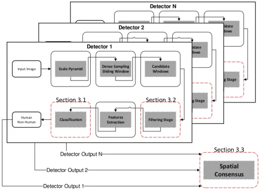
An overview of our methodology is summarized in Figure 3.1, where we show at which stage of pipeline the described method is operating. In Section 3.1, we introduce a

Detector Output 2 Detector Output N

Detector N

Input Image

Human Non-Human

Scale Pyramid Dense Sampling Sliding Window Classification Features Extraction Candidate Windows Filtering Stage Detector 2 Input Image Human Non-Human

Scale Pyramid Dense Sampling Sliding Window Classification Features Extraction Candidate Windows Filtering Stage Detector 1 Input Image Human Non-Human

Scale Pyramid Dense Sampling Sliding Window Classification Features Extraction Candidate Windows Filtering Stage

Section 3.1 Section 3.2

Detector Output 1

Spatial Consensus

Section 3.3

Figure 3.1. Pipeline detection and its respective section. Red dashed lines

denotes where our work operates.

brief mathematical definition of the PLS, the main features of the oblique decision tree and how the oRF-PLS and oRF-SVM are built, respectively. Section 3.2 describes the steps performed by each filtering approach evaluated as well as its properties. Finally,

(34)

14 Chapter 3. Methodology

in Section 3.3, we present our proposed late fusion algorithm to combine multiple detectors.

3.1 Oblique Random Forest with Partial Least

Squares

This section starts by giving a brief mathematical definition of the Partial Least Squares (PLS). Afterwards, we describe the features of the oblique random forest as well as its build process. Last, we describe how to employ the PLS and SVM with the oblique random forest and an adaptive bootstrapping procedure to improve the performance of the oblique random forest.

3.1.1 Partial Least Squares

The PLS is a technique widely employed to model the relationship between variables (features) utilized in several application areas [Rosipal and Krämer, 2006]. A brief definition of the PLS is shown below, detailed mathematical definitions can be found in Wold [1985] and Rosipal and Krämer [2006].

Let X ⊂ Rm _{be the matrix representing} _n _{data in} _m₋_dimensional _{space of} features,y⊂R be the label class, in this work a 1−dimensionalvector. The method decomposes X and y as

X =T PT +E, y=U qT +f, (3.1)

where T and U are n ×p matrices of variables in latent space, p is a parameter of algorithm. P and q corresponds to matrix m×p and vector 1×p of loadings, in this order. The residuals are represented by E and f matrices of size n×m and n×1, respectively. The PLS, constructs a matrix of weight W = {w1, w2, ..., wp}, where

the ith column represents the maximum covariance (cov) between the ith element of the matrix T and U as denotes the Equation 3.2. This procedure is made using the nonlinear iterative partial least squares (NIPALS) algorithm [Wold, 1985].

[cov(ti, ui)]2 = max

wi

[cov(Xwi, y)]2 (3.2)

(35)

3.1. Oblique Random Forest with Partial Least Squares ₁₅

vector, vi. To this end, first we compute the regression coefficients, βm×1,

β =W(PT_W₎−₁

TT_y, _(3.3)

then the regression response to a features vector vi is

yvi = ¯y+β

T

vi, (3.4)

where y¯represents the average of y.

An important aspect of the PLS regarding the traditional dimensionality reduc-tion techniques, e.g, principal component analysis (PCA) [Shlens, 2005], is that it con-siders the class label in the construction process of the matrix of weights W. Schwartz et al. [2009] showed that the PLS is able to separate data better than PCA, in the pedestrian detection context. In view of their results [Schwartz et al., 2009], we opt to utilize the PLS as dimensionality reduction technique as well as regression model.

3.1.2 Oblique Random Forest

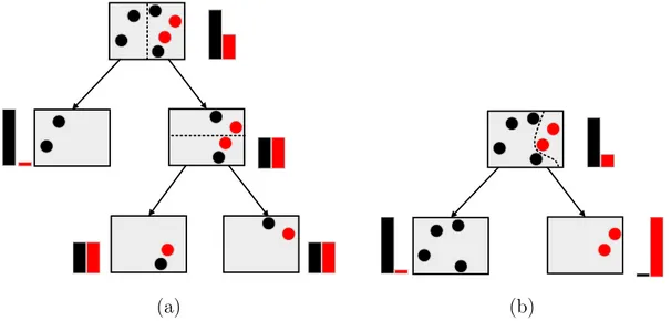
Figure 3.2 illustrates the main advantage provided by oblique random forest (oRF). As can be observed, the samples are separated by oriented hyperplanes (Figure 3.2 (b)), achieving a better partition of the space that induces to shallower trees.

(a) (b)

Figure 3.2. Decision tree split types (the bars represent the information gain).

(a) Orthogonal split, tree with depth 2. (b) Oblique split, tree with depth 1.

(36)

noticed by Breiman [2001] and Criminisi and Shotton [2013], this technique ensures decorrelation (or diversity) between the trees, presenting an important contribution to improve the accuracy. In particular, the bagging mechanism also provides diversity on the random forest [Breiman, 2001]. However, as reported by Criminisi and Shotton [2013], several works are abandoning the use of such method. Therefore, in this work we discard the use of bagging since a considerable number of samples is required to build each oblique decision tree. Second, a starting node (root),Rj, is created with all data. The creation of a node estimates a decision boundary (hyperplane) to separate the presented samples according to their classes. Third, the data samples are projected onto the estimated hyperplane and a thresholdτ is applied on its projected values splitting the samples between in two children (Rjr, Rjl). The samples below this threshold are sent to the left child, Rjl, and samples equal or above to the threshold are sent to its right child,Rjr. This procedure is recursively repeated until the tree reaches a specified depth or another stopping criterion.

To estimate the threshold that better separates the data samples, we employ the gini index as quality measure. The gini index is computed in terms of

∆L(Rj, s) =L(Rj)−|Rjls|

|Rj | L(Rjls)−

|Rjrs |

|Rj | L(Rjrs), (3.5)

where

L(Rj) =

K

X

i=1

lij(1−l j

i), (3.6)

in which s ∈S (S is a set of thresholds), K represents the class number and lj_i is the label of class i at the nodej. We choosegini index because it produces an extremely randomized forest [Criminisi and Shotton, 2013].

Once the trees have been learned, given a testing sample v, each node sends it either to the right or to the left child according to the threshold applied to the projected sample. For a tree, the probability of a sample to belong to class c is estimated combining the responses of the nodes in the path from the root to the leaf that it reaches at the end. The final response for a sample v presented to the forest is given by

l(c|v) = 1

F F

X

i=1

li(c|v), (3.7)

whereF is the number of trees composing the forest.

(37)

3.1. Oblique Random Forest with Partial Least Squares ₁₇

PLS. The value topis set by validation (see Section 4.2.2). Subsequently, the regression coefficients β are estimated using the Equation 3.4. Finally, the best threshold to split the training data samples, is obtained using the gini index on the regression values given by Equation 3.4.

The difference to build the oRF-SVM is that the received data samples do not have their dimensionality reduced and instead computing the regression coefficients, a linear SVM1

is learned at each tree node. The remaining of the process is equal. This way, the approaches can be compared only in terms of better data separation and generalization.

3.1.3 Boostrapping

The idea of bootstrapping consists in retraining an initial model F, using negative sample considered hard to classify (hard negatives samples). These hard negative samples are found according to a threshold applied on the prediction performed by F in a pool of negative examples S. The samples above of this threshold are introduced into a set N. It is important to mention that this set S are negative samples distinct of the negative examples used to generate the initial model F. Once modelF classified

Algorithm 1: Bootstrapping

input : Samples to hard negative miningS, Iterations K

output: Forest F

1 for iteration = 1 until K do

2 Find hard negatives samples (N) in S, using the current forest F. 3 X =P ∪N, where P is the set of positive samples.

4 Train n new trees using X.

5 Add these new trees n into current forest F. 6 iteration=iteration+ 1.

7 end

all the negative examples in S, it is updated using the initial positives samples and the samples in set N. This procedure is repeatedK times. Algorithm 1 is a variation of the bootstrapping proposed by Marín et al. [2013] focused on random forest and summarizes the steps above mentioned. Our experiments (Section 4.2.3) showed that, for each bootstrapping iteration, the log-average miss-rate decreases (lower is better). However, once four iterations are reached, the accuracy saturates.

1

(38)

In particular, our bootstrapping procedure ensures diversity among the trees at the forest, since in each iteration different negative samples are utilized to produce n new trees, as we explained before.

3.2 Filtering Approaches

This section describes each filtering approach and its properties. The following filtering approaches are used in our study: the entropy filter, the magnitude filter, the random filtering and the saliency map based on spectral residual. A common feature among them is illustrated in Figure 3.3, in which all removed regions do not contain the object of interest (in our context, the pedestrian).

(a)Input image (b)Entropy filter

(c) Magnitude filter (d) Saliency map based on spectral residual

Figure 3.3. Translucent areas demonstrate regions eliminated by filtering stage

for different filtering approaches. Some filters removed more regions than others, yet, all preserved the pedestrian (the random filtering, also considered in this work, was not showed since it is difficult to be visualized).

3.2.1 Entropy Filter

(39)

3.2. Filtering Approaches ₁₉

to its more uniform distribution when compared with windows containing a human (rich on edges in a given orientation).

The computation process is the following. Initially, we compute the image deriva-tivesIx′

andIy′

, regarding thexandy, using a3×3Sobel mask [Gonzalez and Woods, 1992]. Then, we estimate the orientation (0◦

to180◦

) for each pixeli using

θi = arctan

Iy′₍_x,y₎

Ix′₍_x,y₎

. (3.8)

Afterwards, we generate a histogram h incrementing its respective bin θi by the mag-nitude of the pixel2

(the number of bins was set experimentally to be nine). Finally, we normalize h using the L1-norm to become a probability distribution and estimate its entropy as

E(w) = −

bins

X

i=0

(a(hi) log(a(hi))), (3.9)

where a(hi) denotes the value of the normalized bin i and E(w) is the entropy to detection window w.

3.2.2 Magnitude Filter

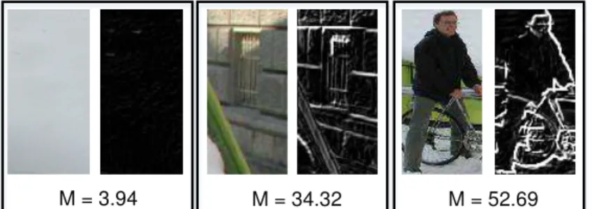
The average of the gradient magnitude within a detection window can be used as a cue for discriminating humans from the background. As illustrated in Figure 3.4, there is a gap between the magnitude values of regions containing background and regions containing humans. Therefore, we can utilize this interval to reject detection windows with background. This is a similar procedure that Singh et al. [2012] employed to discard image patches without relevant information.

2

We accumulate the magnitude to soften the contribution of noisy pixels to h_.

M = 52.69

M = 3.94 M = 34.32

Figure 3.4. Different regions of the image (detection windows) captured by

sliding windows approach and their respective magnitude images whereM _{is the}

(40)

To this filter, we initially compute the image derivatives as in the entropy filter. Then, we sum all values inside the detection window as

M(w) = 1

D X i X j q I2

x′(i, j) +I_y2′(i, j)

, (3.10)

whereD is the window area.

This filter is relatively simple and our experiments demonstrate that a large number of windows can be discarded. Besides, it presents two important aspects: (1) when using integral images, the average magnitude can be computed using only four arithmetic operations yielding a faster filtering stage; (2) the magnitude is a feature widely used to create the image descriptors, such as the HOG, therewith detectors based on such descriptors do not have extra computational cost after this filtering stage.

3.2.3 Random Filtering

The random filtering technique consists in randomly selecting a sufficiently large amount m˜ of windows from the set of detection windows W, which has cardinality m=|W| [de Melo et al., 2014]. The approach relies on the Maximum Search Problem theorem [Schölkopf and Smola, 2002] to ensure that every person will be covered. The theorem provides a set of tools that allows to estimate the required number of windows

˜

m to be selected.

The problem is formulated as follows. Let W = {w1, . . . , wm} be the set of

m detection windows generated by the sliding window approach. In this problem, one needs to find a window wiˆ that maximizes the criterion F[wi], which evaluates whether a detection window covers a pedestrian or not. The problem is usually solved by evaluating each window wi regarding such criteria, thus requiring m evaluations. However, such evaluations are expensive since the number of windows is large. The Maximum Search Problem states that one does not need to evaluate every window. By selecting a random subsetW˜ ⊂W sufficiently large, it is very likely, that the maximum overW˜ will approximate the maximum over W (with a confidence η).

The size m˜ =|W˜| of this random selection can be estimated by

˜

m= log (1−η)

ln (n/m) , (3.11)

(41)

3.2. Filtering Approaches ₂₁

In their initial work, de Melo et al. [2014] proposed an extra stage, the location regression, where each selected windows is displaced by δX and δY adjusting itself better on the pedestrian. Despite this procedure improve the detection performance, the δX and δY values must be previously learned in a training step. Hence, since we are evaluating the random filtering only on the selection stage and the focus of our study is to evaluate simple filtering approaches, we disregard the location regression since it depends on previous learning.

3.2.4 Salience Map based on Spectral residual

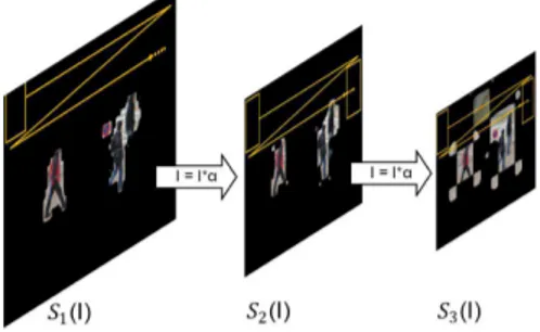
In their work, Hou and Zhang [2007] observed that images share the same behavior when viewed from the log spectral domain. Using this feature, the authors proposed a method to capture the saliency regions of the image removing redundant information and preserving the non-trivial regions in the scene. Following Silva et al. [2012], we ap-ply the saliency map on multi-scales as this procedure outperforms the original method proposed in Hou and Zhang [2007]. Moreover, we demonstrate that the choice of the threshold used to discard regions of the image is essential to reject a large number of detection windows without compromising accuracy.

As mentioned in Chapter 2, the proposed threshold used to consider a detection window valid is based on the global mean of the saliency map. In this work, we propose two alternative thresholds: (1) the amount of the saliency pixels within a detection window is greater or equal to one, and (2) the sum of the saliency pixels within a detection window is greater than 10% of its dimension. In our experimental results, we show that the latter proposed thresholding allows to discard a larger number of candidate windows, without affecting the detection rate.

Figure 3.5. Sliding window approach on saliency map.

(42)

image is downsampled by a scale factor and the process above is repeated, as illustrated in Figure 3.5. In other words, we can consider which each output image of the scale pyramid (see Figure 1.1) is a S(I).

3.3 Spatial Consensus

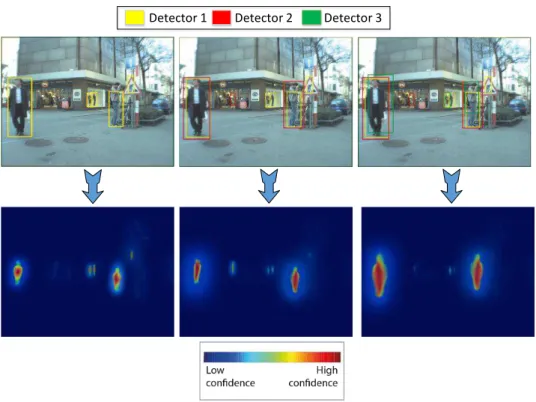
This section describes the steps of our proposed algorithm to combine multiple-detectors iteratively. Using the responses coming from these multiple-detectors, we weight their scores and give, giving more confidence to candidate windows that really belong to a pedestrian (our hypothesis is that regions containing pedestrians have a dense concen-tration of detection windows from multiple detectors converging to a spatial consensus) and eliminating a large amount of false positives, as illustrates Figure 3.6.

Detector 1 Detector 2 Detector 3

Figure 3.6. Detection results and their respective heat map. From the left to

the right. First image only one detector is being used to generate the heat map, but in the second and third images two and three detectors, respectively, are used to generate the heat map. Each bounding box color represents the results of a distinct detector. As can be noticed, the addition of more detectors reduces the confidence of false positives with similar human body structure and reinforces the pedestrian hypothesis (best visualized in color).

(43)

3.3. Spatial Consensus ₂₃

fusion) is to normalize the output scores to the same range because different classifiers usually produce responses in a different ranges. For instance, if the classifier used by the ith detector attributes a score of [−∞,+∞] to a given candidate window and the classifier of the jth detector attributes a score between [0,1], the scores cannot be combined directly. To address this problem, in this work we employ the same procedure used by Jiang and Ma [2015] to normalize the scores. The procedure steps are described as follows. First, we fix a set of recall points, e.g, {1,0.9,0.8,0.7, ...,0}. Then, for each detector, we collect the set of scores, τ, that achieve these recall points. Finally, we estimate a function that projects τj onto τi (details in Section 4.4.1).

After normalizing the scores to the same range, we combine the candidate win-dows of different detectors as follows. Let detroot be the root detector from which the window scores will be weighted based on the detection windows of the remaining de-tectors in {detj}n

j=1. For each window wr ∈ detroot, we search for windows wj ∈ detj

that satisfies a specific overlap according to the Jaccard coefficient given by

J = area(wr∩wj)

area(wr∪wj), (3.12)

wherewr andwj represent windows ofdetroot anddetj, respectively. Finally, we weight wr in terms of

score(wr) =score(wr) +score(wj)×J. (3.13)

The process described above is repeated n times, where n is the number of detectors besides the root detector. Algorithm 2 represents the aforementioned process.

Regarding the computational cost, the asymptotic complexity of our method is denoted by

O(cwroot× n

X

j=1

cwj) =O(cwroot×p) =O(cw2),

where cwroot is the number of candidate windows ofdetroot,cwj denotes the number of detection windows of the jth detector andpis the amount of all candidate windows in {detj}n

j=1. Similarly, the approach proposed by Jiang and Ma [2015] (weighted-NMS

method) presents complexity of O(cwlogcw+cw2₎_{. Although both methods present}

a quadratic complexity, p is extremely low because the non-maximum suppression is employed for each detector before presenting the candidate windows to Algorithm 2 (see Section 4.4.10), which renders the computational cost of both our Spatial Con-sensus method and the baseline approach [Jiang and Ma, 2015] to be negligible when compared with the execution time of the individual pedestrian detectors.

(44)

Algorithm 2: Spatial Consensus

input : Candidate windows of detroot and {detj}n j=1

output: Updated windows of detroot

1 for j ←1 to n do

2 project detj score todetroot score; 3 foreach wr in detroot do

4 foreach wj in detj do

5 compute overlap using Equation 3.12; 6 if overlap >=σ then

7 update wr score using Equation 3.13;

8 end

9 end

10 if wr does not presents any matching then

11 discardwr;

12 end

13 end

14 end

main aspects: (1) instead of inserting the candidate windows of detroot and detj into a single set and performing weighted-NMS (see Section 4.4.3), we fix detroot and weight its windows using the detj windows responses. In this way, we reduce the possibility of errors added by choosing a window that covers poorly the pedestrian according to the ground-truth, as illustrated in Figure 3.7 (a) - the suppression made by weighted-NMS algorithm, the chosen window will be the orange and thus we lose the pedestrian, generating one false positive and one false negative; (2) in the weighted-NMS [Jiang and Ma, 2015], windows without overlap will be kept, as illustrated the Figure 3.7 (b). On the other hand, our approach (step 11 in Algorithm 2) remove such a window even if it presents high confidence score. This is the key point that enables our approach to be powerful in eliminating hard false positives.

3.3.1 Removing the Dependency of the Root Detector

According to the algorithm described in the previous section, the execution of the SC algorithm requires the selection of a root detector. To address this restriction, we propose a generation of a “virtual” root detector, referred to as virtual root detector. The idea behind building this virtual root detector is to increase the flexibility of the algorithm – this way, we do not need to specify a particular pedestrian detector as input to the SC algorithm (see Algorithm 2).

(45)

3.3. Spatial Consensus ₂₅

set of detectors {detj}n

j=1. For a detection window w

j

i ∈ detj with dimensions (x, y, width, height), we search for overlapping windows in the remaining detectors (wl

i, l = 1,2, ..., k) to create a set of windows that will be used to generate a single window belonging to the detvr using

wvr i =

1

k k

X

l=1

wl

i, (3.14)

where k is the number of overlapping windows to the window wij. Finally, we assign a constant C (for instance, C = 1) to this novel window. This constant contains the score of this window and its value will be updated after executing the SC algorithm.

Once the windows of the virtual root detector had been generated, we can execute the SC algorithm. However, the steps 10 to11 of the algorithm are inoperative, since we will always have windows presenting overlapping.

Score: 0.89

Score: 0.75

Score = 0.9

Score = 0.7 Score = 0.8

(a) (b)

Figure 3.7. Different aspects between our proposed Spatial Consensus algorithm

and the weighted-NMS [Jiang and Ma, 2015]. Yellow and orange boxes indicate the detection coming from det_root _and det_j_{, respectively, and the dashed green}

box shows the ground-truth annotation. (a) Our Spatial Consensus algorithm will maintain the yellow box (true positive), since this window belongs to det_root_,

(46)

(47)

Chapter 4 Experimental Results

We start this chapter describing the benchmarks employed through of our work. Then, we present the experiments, results and discussion regarding the oRFs, filtering ap-proaches and spatial consensus, respectively.

The majority of the methods were implemented using the Smart Surveillance Framework (SSF) [Nazare et al., 2014], except to generate the saliency map (see Section 3.2.4), where we use its version that is available online1

.

To measure the detection accuracy, we employed the standard protocol evalua-tion used by state-of-the-art called reasonable set (a detailed discussion regarding this protocol of evaluation can be found in [Dollár et al., 2009; Dollár et al., 2012]), in which only pedestrians with at least 50 pixels high and under partial or no occlusion are considered. The reasonable set measures the log-average miss rate of the area un-der the curve on the interval from 10−2

to 100 _{(low values are better). However, in}

some experiments, we report the results using the interval from10−₂

to10−₁

. The area under curve in this interval represents a very low false positive rate (that is a require-ment to real applications, e.g., surveillance, robotics and transit safety), this way, we evaluate the methods under a more rigorous detection. We used the code available in the toolbox2

of the Caltech pedestrian benchmark to perform the evaluations.

4.1 Datasets

We compare our work with the state-of-the-art methods on three challenging widely-used pedestrian detection benchmarks: INRIA Person, ETH and Caltech. An extra dataset was used as validation set (TUD pedestrian) to calibrate the oRF parameters.

1

http://www.saliencytoolbox.net/ 2

www.vision.caltech.edu/Image_Datasets/CaltechPedestrians/

(48)

28 Chapter 4. Experimental Results

However, we prefer not report the results of the other methods in this dataset since it is more utilized to pedestrian detectors that are part based [Andriluka et al., 2008].

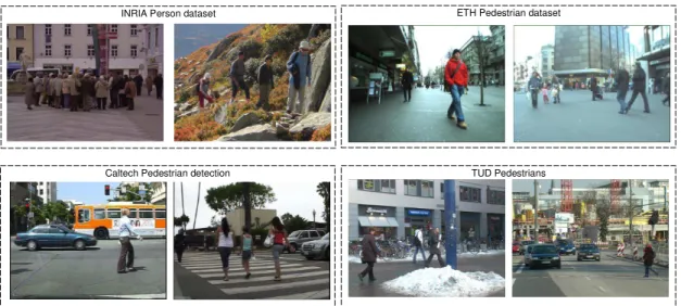
Figure 4.1 illustrates the different scenarios of the datasets. As can be noticed, the datasets present high variability in the terms of illumination, human pose and background, rendering the pedestrian detection a challenging task.

INRIA Person dataset ETH Pedestrian dataset

Caltech Pedestrian detection TUD Pedestrians

Figure 4.1. Image examples from the datasets used in this work.

INRIA Person dataset. Proving rich annotations and high quality images, INRIA Person dataset still remains as the most employed dataset in pedestrian detection [Dalal and Triggs, 2005]. This dataset provides both positive and negative sets of images for training and testing, where there is a wide variation in illumination and weather conditions.

ETH Pedestrian dataset. Composed of images with size 640×480 pixels, the ETH dataset provides stereo information. In this dataset are available four video sequences, one for training and three for test [Ess et al., 2007]. The large pose and people height variation make this dataset a challenging pedestrian detection dataset.

Caltech Pedestrian detection. Nowadays, this is the most predominant and chal-lenging benchmark in pedestrian detection. Caltech dataset consists of urban environ-ment images acquired from a moving vehicle [Dollár et al., 2012]. This dataset provides about 50,000 labeled pedestrians. Moreover, it has been largely utilized by methods designed to handle occlusions since such labels are available.

(49)

4.2. Oblique Random Forest Evaluation ₂₉

composed from people of side view, we are using this dataset as validation set (only to the experiments of the oRFs), aiming at measure the power of generalization of the models by considering that they were learned on side view samples.

4.2 Oblique Random Forest Evaluation

This section details the experimental setup utilized to validate our proposed oblique random forest as well as the comparison between our method with the baseline and the state-of-the-art.

4.2.1 Feature Extraction

We extract the HOG descriptor for each detection window following the configuration proposed by Dalal and Triggs [2005], with blocks of 16×16pixels and cells8×8pixels. This configuration results in a descriptor of 3780dimensions. We are using these 3780

features during the feature selection process (see Section 3.1.2), for both the oblique random forest to provide a comparison not influenced by the features.

4.2.2 Tree Parameters

To tune the parameters for both oRFs, we adopted the grid search technique where each parameter is placed as a dimension in a grid. Each cell in this grid represents a combination of the parameters.

(50)

sub-30 Chapter 4. Experimental Results

stantially. For instance, modifying p from 6 to 8 the log-average miss rate goes from

38.18% to42.98%. Therefore, this is a crucial parameter to oRF-PLS.

It is important to mention that the number of trees composing the forest is considering bootstrapping iterations (see Section 3.1.3).

4.2.3 Bootstrapping Contribution

As can be noticed in Figure 4.2, the log-average miss rate presents a significant reduc-tion to each bootstrapping iterareduc-tion. From the initial model to the third iterareduc-tion, the log-average miss rate decreases 16 percentage points (p.p) to oRF-PLS against 17.43

p.p. to oRF-SVM. This improvement is achieved since in each bootstrapping iteration, the forest finds more hard negative samples and these examples, when used to produce more trees, allow the current forest be more robust to false positives. In addition, for each bootstrapping iteration, the computational cost increases since the forest becomes larger, hence, more projections are performed.

10−2 10−1 100

.20 .30 .40 .50 .64 .80

false positives per image

miss rate

54.18% Initial Model 39.30% Iteration 1 39.10% Iteration 2 38.18% Iteration 3

10−2 10−1 100

.20 .30 .40 .50 .64 .80 1

miss rate

59.10% − Initial model 50.22% − Iteration 1 45.71% − Iteration 2 41.67% − Iteration 3

(a) oRF-PLS (b) oRF-SVM

Figure 4.2. Log-average miss rate achieved in each bootstrapping iteration using

oRF-PLS and oRF-SVM, respectively, on validation set.

4.2.4 Influence of the Number of Trees

(51)

4.2. Oblique Random Forest Evaluation ₃₁

8 16 24 32 40 200

0 10 20 30 40 50 60 70 80 NumberSofStrees Log − averageS missS rat eS (%) oRF−PLS oRF−SVM

Figure 4.3. Log-average miss-rate (in percentage points) on the validation set

as a function of the number of trees.

high (see Section 4.2.5). In addition, by computing the standard deviation of the log-average miss rate, we can notice that the oRF-SVM is more sensitive to variation of the number of trees to presenting a standard deviation of 10.58% while our proposed method presented a standard deviation of2.42%. Thus, the use of PLS to build oRF is more adequate than use the SVM since it produces smaller and more accurate forests.

4.2.5 Time Issues

In this experiment, we show that the proposed oRF-PLS is faster than oRF-SVM. For this purpose, we performed a statistical test (visual test [Jai, 1991]) among the time (in seconds) to run the complete pipeline detection on an image of640×480 pixels. To each approach, we execute the pipeline 10 times and compute its confidence interval using95%of confidence. The oRF-PLS obtained a confidence interval of[270.2,272.44]

against [382.72,392.72] achieved by the oRF-SVM. As can be observed, the confidence intervals does not overlap, showing that the methods present statistical differences regarding the execution time, being the proposed method faster.

4.2.6 Comparison with Baselines

(52)

outper-32 Chapter 4. Experimental Results

forms a robust partial occlusion method, HOG+LBP [Wang et al., 2009], in 1.84and

6.28 percentage points to the area in10−₂

to100 _and ₁₀−₂

to 10−₁

, respectively.

When evaluated on the ETH pedestrian dataset, showed in the second row in Fig-ure 4.4, the accuracy of our method decreases. However, its result still overcomes the oRF-SVM in 2.35 and 2.99 percentage points on the area in 10−₂

to 100 _and ₁₀−₂

to

10−1

, respectively.

According to results showed in this section, the proposed oRF-PLS is able to obtain equivalent (or better) results when compared with traditional classifiers.

10−2 10−1 100

.20 .30 .40 .50 .64 .80

miss rate 48.17% oRF−SVM 45.98% HOG 40.09% Pls 39.10% HogLbp 37.26% oRF−PLS

10−2 10−1

.40 .50 .64 .80

miss rate

64.14% oRF−SVM 61.70% HOG 54.87% HogLbp 53.20% Pls 48.59% oRF−PLS

(a) (c)

INRIA Person Dataset

10−3 10−2 10−1 100 101 .05 .10 .20 .30 .40 .50 .64 .80 1

miss rate 69.75% oRF−SVM 67.40% oRF−PLS 64.23% HOG 54.86% Pls 55.18% HogLbp

10−2 10−1

.40 .50 .64 .80

miss rate 76.73% oRF−SVM 79.55% HOG 73.74% oRF−PLS 70.89% Pls 68.91% HogLbp (b) (d)

ETH Pedestrian Dataset

Figure 4.4. Comparison of our oRF-PLS approach with the state-of-the-art.

The first column reports the results using the log-average miss-rate of10−₂

to100

(standard protocol). The second column report the results using the area of10−₂

to 10−₁

(53)

4.3. Filtering Approaches ₃₃

4.3 Filtering Approaches

In this section, we evaluate several aspects of the filtering approaches and describe the experimental setup employed throughout of our analyze.

4.3.1 Scaling Factor Evaluation

Pedestrians can have different heights in an image due to their distance to the cam-era [Dollár et al., 2012]. Therefore, to ensure that all people have been covered by detection windows, a common technique is to employ a pyramid scale, keeping fixed the sliding window size. To generate this pyramid, we employ an iterative procedure that scales the image by a scale factor α, in which the new image is generated by ap-plying this scale factor to the previously generated image. In the first experiment, we

1.15 1.10 1.05 1.01

0 1 2 3 4 5 6xd10

5

35,364 48,495

95,887

519,851

ScaledFactor

Numberd

of

dwindowsd

produced

Figure 4.5. Tradeoff between scale factor and number of windows generated for

a 640_×480_image.

evaluate the impact of the scaling factor on the number of detection windows generated, as well as the miss rate obtained by the detectors.

Figure 4.5 shows that the number of windows increases quickly depending on α. For a 640×480 image, while the sliding window algorithm generates 10 scales with α = 1.15, this number increases to 171 scales when α = 1.01. Table 4.1 presents the results achieved by the detectors at100_{false positive per image (FPPI), value commonly}

used to report the results in pedestrian detection [Dollár et al., 2012; Benenson et al., 2014].

(54)

Table 4.1. Miss rate obtained at 100 _{FPPI with different scale factors.}

Scale factor α HOG+SVM PLS+QDA oRF-PLS oRF-SVM

1.15 0.34 0.33 0.28 0.26

1.10 0.33 0.29 0.28 0.24

1.05 0.31 0.29 0.27 0.23

1.01 0.29 0.27 0.25 0.22

part of the generated windows will be removed in the filtering stage and will not be presented to the classifier. However, throughout of the next experiments, we are using α= 1.15, since it is a typical value used in pedestrian detection [Benenson et al., 2014] and, this way, our results can be compared directly with the original detectors.

4.3.2 Saliency Map Threshold

Our next experiment evaluates the power of the saliency map to discard candidate windows using different threshold approaches (as discussed in Section 3.2.4). According to the results showed in Figure 4.6, the proposed threshold approach is able to discard a larger number of detection windows, demonstrating to be more suitable than the threshold approach proposed in [Hou and Zhang, 2007]. It is important to mention that all the thresholds evaluated have been set to achieve the same recall to provide a fair comparison. 0 5 10 15 20 25 30 35 40 45 50 55 127 307 487 P erce nt ageH of Hdiscar dH (7) WindowHintensityH>H1pixel HouHandHZhangH[2007] WindowHintensityH>H107

Figure 4.6. Threshold approaches analyzed to be used as rejection criteria in

(55)

4.3. Filtering Approaches ₃₅

4.3.3 Number of Discarded Windows

Figure 4.7 presents the percentage of rejected windows achieved by the filters assuming that an ideal detector3

were to be used afterwards. In this experiment, we fixed α as

1.15, which generated a total of15,956,718detection windows for all testing images of the INRIA person dataset. One may notice that some filters were able to reject more than 30%, while preserving the same recall rate as obtained without window rejection. According to the results in Figure 4.7, the entropy filter was able to reject a small number of windows when compared to the other filters. Besides, this filter presented the largest increase of miss rate when a larger percentage of detection windows were dis-carded. The magnitude filter demonstrated to be effective to discriminate background windows from humans. It was able to reject up to 50% of the candidate windows con-serving the recall rate above 90%. The random filtering and saliency map presented a powerful ability to reject candidate windows, discarding around 70%while keeping the recall rate above of 90%.

0 0.1 0.2 0.3 0.4 0.5 0.6 0.7 0.8 0.9 1

0 0.1 0.2 0.3 0.4 0.5 0.6 0.7 0.8 0.9 1 PercentageuDiscarded Recall Entropy Magnitude RandomuFiltering SaliencyuMap

Figure 4.7. Relationship between rejection percentage and recall achieved by

filters (assuming that an ideal detector was employed after the filtering stage).

4.3.4 Filtering Approaches Coupled with Detectors.

Our last experiment regarding the filtering approaches evaluates the distinct behavior of the filters when employed before different detectors. First, we defined ranges of rejection percentages (30−40,41−50and 51−60). We use these ranges to determine

3

(56)

Table 4.2. Miss rate at 100 _{FPPI applying the filtering stage on the}

detec-tors. Values between parentheses indicate the percentage of discarded detection windows.

Entropy Magnitude R. Filtering S. Map

HOG+SVM

0.39(31%) 0.34(38%) 0.36(32%) 0.33(38%) 0.45(41%) 0.35(44%) 0.36(45%) 0.34(48%) 0.58(53%) 0.38(54%) 0.37(53%) 0.34(52%)

PLS+QDA

0.36(31%) 0.33(38%) 0.33(32%) 0.30(38%) 0.42(41%) 0.34(44%) 0.35(45%) 0.30(48%) 0.56(53%) 0.36(54%) 0.35(53%) 0.31(52%)

oRF-PLS

0.31(31%) 0.28(38%) 0.30(32%) 0.26(38%) 0.38(41%) 0.30(44%) 0.30(45%) 0.27(48%) 0.51(53%) 0.31(54%) 0.30(53%) 0.28(52%)

oRF-SVM

0.30(31%) 0.27(38%) 0.28(32%) 0.25(38%) 0.37(41%) 0.29(44%) 0.29(45%) 0.25(48%) 0.51(53%) 0.31(54%) 0.28(53%) 0.25(52%)

the same rejection ratio among the filters, since we are only interested in analyzing the relationship between filter and detector. We reported the miss rate fixed at 100

FPPI. The results are reported in Table 4.2. In the evaluation of the number of discarded windows, the random filtering outperformed all approaches. However, in this experiment, the detectors performed poorly when evaluating the windows selected by this approach. This happens due to its random essence, since windows that fit the pedestrian might be slightly misplaced from the pedestrian’s center. Hence, as holistic detectors are trained considering a centered window, the classifier assigns a low score to that sample, even though it satisfies the evaluation protocol.

The results obtained indicate that for a fixed recall (Figure 4.7), each filter is able to reject a percentage distinct of candidate windows, being the saliency map the most efficient since it is able to discard a large number of candidate windows and reduce the miss rate. Moreover, when more windows are discarded, the detectors are effected differently according to filter being applied.

The Good, The Fast And The Better Pedestrian Detector

THE GOOD, THE FAST AND THE BETTER

ARTUR JORDÃO LIMA CORREIA.

THE GOOD, THE FAST AND THE BETTER

PEDESTRIAN DETECTOR

Orientador: William Robson Schwartz

Belo Horizonte

ARTUR JORDÃO LIMA CORREIA.

THE GOOD, THE FAST AND THE BETTER

PEDESTRIAN DETECTOR

Advisor: William Robson Schwartz

Belo Horizonte

Acknowledgments

Resumo

Abstract

List of Figures

List of Tables

Contents

Chapter 1

Introduction

1.1

Motivation

1.2

Objectives

1.3

Contributions

1.4

Work Organization

Chapter 2

Related Work

Chapter 3

Methodology

3.1

Oblique Random Forest with Partial Least

Squares

3.1.1

Partial Least Squares

3.1.2

Oblique Random Forest

3.1.3

Boostrapping

3.2

Filtering Approaches

3.2.1

Entropy Filter

3.2.2

Magnitude Filter

3.2.3

Random Filtering

3.2.4

Salience Map based on Spectral residual

3.3

Spatial Consensus

3.3.1

Removing the Dependency of the Root Detector

Chapter 4

Experimental Results

4.1

Datasets

4.2

Oblique Random Forest Evaluation

4.2.1

Feature Extraction

4.2.2

Tree Parameters

4.2.3

Bootstrapping Contribution

4.2.4

Influence of the Number of Trees

4.2.5

Time Issues

4.2.6

Comparison with Baselines

4.3

Filtering Approaches

4.3.1

Scaling Factor Evaluation

4.3.2

Saliency Map Threshold

4.3.3