Ficha catalográfica elaborada pela Biblioteca Mario Henrique Simonsen/FGV
Pires, Victor Duarte Garcia
Monetary policy and the cross-section of stock returns: a FAVAR approach / Victor Duarte Garcia Pires. – 2012.
18 f.
Dissertação (mestrado) - Fundação Getulio Vargas, Escola de Pós-Graduação em Economia.
Orientador: Tiago Couto Berriel. Inclui bibliografia.
1. Política monetária. 2. Bolsa de valores. I. Berriel, Tiago Couto. II. Carvalho, Carlos Viana de. III. Fundação Getulio Vargas. Escola de Pós- Graduação em Economia. IV. Título.
Funda¸c˜ao Get´ulio Vargas
Escola de P´os-Gradua¸c˜ao em Economia - EPGE
Monetary Policy and the Cross-section of Stock Returns
A FAVAR Approach
Disserta¸c˜ao submetida `a Escola de P´os-Gradua¸c˜ao em Economia da Funda¸c˜ao Get´ulio Vargas como requisito de obten¸c˜ao do t´ıtulo de
Mestre em Economia
Aluno: Victor Duarte Garcia Pires Orientador: Tiago Couto Berriel Co-orientador: Carlos Viana Carvalho
Funda¸c˜ao Get´ulio Vargas
Escola de P´os-Gradua¸c˜ao em Economia - EPGE
Monetary Policy and the Cross-section of Stock Returns
A FAVAR Approach
Disserta¸c˜ao submetida `a Escola de P´os-Gradua¸c˜ao em Economia da Funda¸c˜ao Get´ulio Vargas como requisito de obten¸c˜ao do t´ıtulo de
Mestre em Economia
Aluno: Victor Duarte Garcia Pires
Banca Examinadora:
Tiago Couto Berriel (EPGE-FGV/RJ) Carlos Viana Carvalho (PUC/RJ) Marco Bonomo (EPGE-FGV/RJ)
Abstract
We use a factor-augmented vector autoregression (FAVAR) to estimate the impact of mon-etary policy shocks on the cross-section of stock returns. Our FAVAR combines unobserved factors extracted from a large set of financial and macroeconomic indicators with the Federal Funds rate. We find that monetary policy shocks have heterogeneous effects on the cross-section of stock returns. These effects are very well explained by the degree of external finance dependence, as well as by other sectoral characteristics.
Contents
1 Introduction 5
2 Empirical Framework 7
3 Data 8
4 Results 9
4.1 Heterogeneous Responses . . . 9
4.2 Rajan-Zingales Measure of Dependence on External Finance . . . 9
4.3 Market capitalization(Size) and value indices . . . 12
4.4 Identified Shock . . . 15
4.5 VAR vs FAVAR dynamics . . . 16
5 Do the Fama-French Factors matter for monetary policy? 18 5.1 Other specifications and robustness . . . 20
1
Introduction
Measuring the real effects of monetary policy is a central issue in Macroeconomics. Under-standing how central banks actions can influence important macroeconomic variables such as inflation, unemployment, aggregate investment and GDP growth is essential to make good pol-icy decisions. Moreover, the fact that all over the world stock markets participants attentively monitor central banks movements suggest that maybe monetary policy has impact on stock returns as well. The purpose of this paper is to empirically answer this very question: does monetary policy affect stock returns? As suggested by a vast theoretical literature on the lend-ing and balance sheet channels of monetary policy(e.g. Bernanke and Blinder (1992), Hart and Moore (1998) and Gertler and Gilchrist (1994))the presence of capital market imperfections should cause monetary policy to have greater impact on borrowers that are more dependent on external finance. Accordingly, one may expect firms with limited access to capital markets to suffer more from a contractionary monetary policy shock. Indeed, a financially constrained firm may be unable to raise enough capital to invest at its optimal level, therefore damaging its future cash flows, profits and ultimately its dividends. As theory posits that stock prices reflect the discounted present value of the sum of future dividends, following a negative monetary policy shock rational investors would anticipate this future dividends decline and this should readily hurt stock prices.
The empirical attempts to verify this prediction have focused on two general approaches. The first, pioneered by Thorbecke (1997), uses vector auto regressions including a few relevant macroeconomic variables and identifies monetary policy shock as innovations in the monetary policy instrument, usually the Federal Funds Rate. In this study, for each portfolio studied, Thorbecke runs a 7 variable VAR in which the seventh variable is the return of the aforemen-tioned portfolio. Of course this leads to as many identified shocks and dynamical models as portfolios included in the analysis, so when comparing different responses from different port-folios, one is actually using different models to compare the results. The second approach, as in Bernanke and Kuttner (2005), consists of regressing stock returns on a measure of “unan-ticipated monetary-policy action”, ignoring all other macroeconomic variables that could, in principle, be important in pricing stocks. Both approaches find that monetary policy indeed impact equity returns and this happens in an heterogeneous way, that is, different portfolios react quantitatively differently to a monetary shock.
(FAVAR) to identify monetary policy shocks and estimate their effects on stock prices. This approach allows us to consistently exploit the information contained in hundreds of macroeco-nomic and financial time series. If the Federal Reserve and market participants are not wasting time and resources in gathering and analysing this data, it should contain relevant information that is missing in ordinary small-scale VARs. As argued by Bernanke et al.(2005) and Boivin
et al.(2009), using more of the available information reduces the risk of misspecification in the statistical model of the economy. In addition, contrary to simple regressions of stock returns on monetary policy surprises, the VAR approach allows us to trace out the dynamics of stock prices in the periods after the shocks. One could argue that if markets are efficient, than all relevant stock price changes following a monetary shock should take place immediately after the shock, so there is no need to analyse the returns responses months after the shock. We, however, take an agnostic view of the efficiency of the stock market and let the data speak for itself. Finally, after identifying the monetary policy shock, we are able to compute the impulse response for every single portfolio/stock return included in our large dataset. This is paramount since our goal is to estimate and understand the effects of monetary policy shock in the cross-section of stock returns. Note that this is done within the same single framework. There is no need the set up several models to analyse several portfolios.
We find that monetary policy shocks have heterogeneous effects on the cross-section of returns. We then analyze the impulse response functions of portfolios sorted according to 5 characteristics: industry, size (market capitalization), book-to-market ratio, earnings-to-price ratio, and cash-flow-to-price ratio. We also examine the correlation of the responses of industry stock returns with their Rajan-Zingales measure of dependence on external finance (Rajan and Zingales (1998)). We chose these characteristics because all of them serve as proxies for financial constraints.
Take size, for instance. As collateral values are known to alleviate financial frictions, it is reasonable to suppose that bigger firms are less financially constrained. Also, as value stocks are more likely to be financially constrained, one may expect firms with high book-to-markets, earnings-to-price and cash flow-to-price ratios to be more vulnerable to monetary policy shocks. Overall, our results show that the pattern of stock-price responses to monetary shocks across sectors is very well explained by the degree of all these proxies for external finance dependence. This relation is remarkably strong and robust and for the market capitalization proxy.
the analysis. Section 3 describes the data. Section 4 presents the results for the baseline framework. In section 5 we impose the Fama-French Factors as observable components and section 6 concludes.
2
Empirical Framework
We use the same framework described in Boivinet al.(2009). For a more detailed discussion on this econometric tool we also refer the reader to Bernankeet al. (2005) and Stock and Watson (2002).
Suppose the economy is driven by a vector of components Ct whose dynamics is given by
Ct = Φ(L)Ct−1+vt (1)
where
Ct=
Ft Yt
and Φ(L) is finite order lag polynomial. Yt is a M ×1 vector of observed components, Ft
is a K ×1 vector of unobserved components, called factors, and the vector od shocks vt is
assumed to be i.i.d. with mean zero. The factors are supposed to capture the general concepts like ”economic activity”, ”inflation” and ”unemployment”, that cannot be tied to a single time series without a certain degree of arbitrarity. Note that if K = 0 then we have an ordinary VAR, hence the name ”factor-augmented” VAR. As in Boivin et al.(2009), we parsimoniously take Yt to be a single monetary policy instrument, namely the federal funds rate: Yt =Rt
1
. Since (by definition) we cannot observeFt, we need more information to estimate this dynamic
model.
We assume that we have available a large number of economic variables stacked in a panel
X whose dynamics is given by
Xt = ΛCt+et (2)
where et contains series specific components uncorrelated with Ct and are allowed to be
se-rially correlated and weakly correlated across indicators. Equation (2) is called observational equation.
1
We use the two stages estimation described in Stock and Watson (2002). In this procedure, the estimator of F is a weighted averaging estimator, in which the weight is the eigenvectors matrix of the sample variance matrix. The estimation proceeds in the following steps: First, we take F0
t to be the first K principal components of Xt.With these components we can estimate
the loading factor Λ0
= [λ0
F λ
0
R] T
in equation (2)´, and then define X0
t ≡ Xt−λ
0
RRt. Next,
we take F1
t to be the first K principal components of X
0
t and iterates this procedure until a
certain convergence criterion is met. We do so because we are interested in uncovering the space spanned by the factors, that is, the components but the monetary policy instrument,Rt.
Once we uncover the factors by this iteration, we can deal with Ftas if they were
measure-ments and hence estimate equation (1), the dynamic equation, as a standard VAR.
In order to analyze the effects of monetary policy shocks it remains to identify the shock to the federal funds rate. This is done by assuming that all factors respond with a lag to monetary policy changes. Note that this assumption by no means implies that the economic variables in
Xcannot respond instantaneously to a monetary shock. Bernanke et al.(2005) shows that this identification produces plausible results.
3
Data
The data consists of a panel of 781 monthly observations ranging from 1976:1 to 2005:6. We chose this time span so we could use all data used in Boivinet al. (2009), which is publicly and readily available at the American Economic Association website.2
This includes a comprehen-sive set of macroeconomic time series that we believe to be important for a study on monetary policy and stock returns, like several series on output, employment, housing sales, stock prices, exchange rates, interest rates, price indices and disaggregated series on personal consumption expenditures and producer price indices. As we are interested in measuring the effects of mone-tary policy in many portfolios, we augmented this panel by including time series for 49 industry returns, the Fama-French Factors, and portfolios sorted by size, book-to-market, cash flow-to-price, and earnings-to-price ratios. All the later time series were taken from Kenneth French’s website.
4
Results
4.1
Heterogeneous Responses
We begin the analysis examining the impact of a monetary policy shock on industry portfolios excess returns. Figure 1 shows the accumulated response(percent) of 49 industry portfolios to a 25 basis points surprise increase in the Federal Funds Rate, as well as the whole market returns response(dashed black line). This market index is a value weighted average of all NYSE, AMEX, and NASDAQ firms. From this plot it’s clear that the shock’s impact on market excess return is nil at the time of the shock, but there is a large heterogeneity in industries’ responses. Interestingly, this impact becomes pronounced one month after the shock and reaches it’s peak around 4 months after the shock. At that time the accumulated excess returns of the 49 industry portfolios ranges from -10 basis points, for the Drugs industry, to -143 basis points, for the Gold industry. This cross section averages -82 basis points and has a 31 basis points standard error. All these information confirms the existence of heterogeneity on the effects of monetary policy shocks on stock returns. The red solid line is the unweighted average of these 49 portfolios.
4.2
Rajan-Zingales Measure of Dependence on External Finance
Once we verified that stocks respond differently following a monetary shock, a natural next step in our analysis is to relate these heterogeneous responses to sectoral characteristics. We begin by analysing the relation of industries portfolios responses to their Rajan-Zingale measure on dependence on external finance. Rajan and Zingales (1998) define it as capital expenditures minus cash flows from operations divided by capital expenditures. To aggregate these ratios and make them comparable across industries and time, they sum those ratios for every firm over the 1980’s and define the industry dependence on external finance as the median of all firms DEFs in this industry. Evidently, what this measure captures is not exactly the desired amount of external funds, but only the equilibrium that emerges from supply and demand.
As we gathered this measure from the original paper and did not make the calculations ourselves3
, we have this data for just 36 industries. Of these, only 9 industries coincide with
3
Figure 1: Impact of a monetary shock on a cross-section of portfolios.
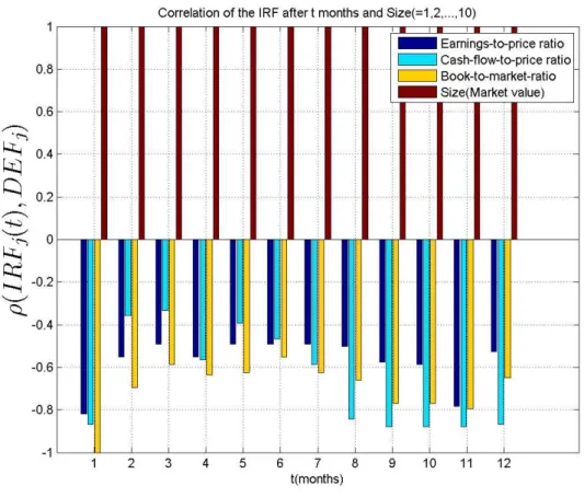
the 49 industries for which we have impulse response functions, which leaves us with the small amount of 9 industry sectors to analyze. The response of these industries portfolios are plotted in Figure 2. With the notable exception of the Drugs industry, we observe a clear correlation between those responses and its corresponding Rajan-Zingales measure. Indeed, if we consider the Drugs industry an outlier and calculate the order correlation of the impact effect of the monetary shock and its RZ DEF it rises(in absolute value) from 0.38 to 0.97. This correlation is 0.37 four months after the shock if we keep the Drugs industry and 0.95 if we discard it. The small number of industries for which we have the Rajan-Zingales measure of DEF however, prevents us from telling if the Drugs industry is an outlier or not. Therefore we are unable to draw any decisive conclusion by analyzing just those 9 industries.
4.3
Market capitalization(Size) and value indices
Figure 2: Impact of a monetary shock on a cross-section of portfolios sorted by industry sector.
for the entire time horizon plotted. This indicates that, when calculating the whole market return, greater weight is put on the stocks less impacted by the monetary shock, or equivalently, bigger stocks are less sensitive to this identified monetary policy shock.
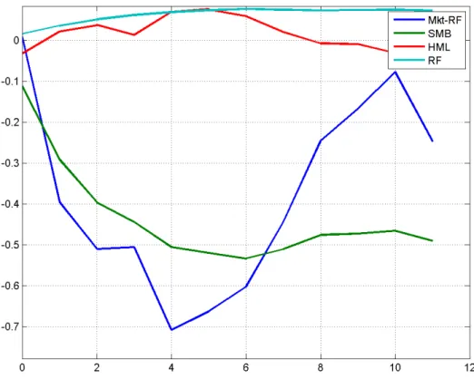
Figure 3: Impact of a monetary shock on the Fama-French Factors.
Figure 4 plots the impulse response functions for 10 portfolios sorted by size and presents our most striking result. Sectors with higher Market Values are plotted with thicker lines. We find a perfectly monotonic relation between market capitalization and stocks excess returns. Immediately after the shock all but the bigger stocks have a negative impact. Note that this is not inconsistent with previous results that a monetary shock has no immediate impact on market excess returns, since the largest caps have overwhelming weight on market indices. All portfolios reach their (negative) peaks 4 months after the shock, ranging from -51 basis points for the highest decile down to -133 basis points for the lowest decile. Furthermore, we note that the correlation of excess returns and size remains very high thought the entire time horizon of the plot.
Figure 4: Impact of a monetary shock on a cross-section of portfolios sorted by Size.
4.4
Identified Shock
A common critique (e.g. Rudebusch (1998) ) of the VAR approach to measure the effects of monetary policy is that the estimated interest rate shocks from different VARs fail to agree among themselves. Is our FAVAR framework subject to this critique? To answer this question we compare the estimated shocks for several model setups. The first is our benchmark model, with the just the Federal Funds Rate as observed component. The second FAVAR model is the one in Boivin et al. (2009). We compare the shocks of these two models with ten standard VAR models that include the growth rate of industrial production, an inflation rate, the log of a commodity price index, the federal funds rate, the log of nonborrowed reserves, the log of total reserves, and the returns of thekth
Figure 5: Correlation between impact and proxies for dependence on external finance.
Benchm. BGM VAR 1 VAR 2 VAR 3 VAR 4 VAR 5 VAR 6 VAR 7 VAR 8 VAR 9 VAR 10
Benchm. 1.00 0.99 0.69 0.70 0.70 0.70 0.70 0.69 0.70 0.69 0.69 0.69
BGM 0.99 1.00 0.70 0.71 0.71 0.71 0.71 0.70 0.71 0.71 0.71 0.71
VAR 1 0.69 0.70 1.00 1.00 0.99 0.99 0.98 0.98 0.98 0.97 0.97 0.96
VAR 2 0.70 0.71 1.00 1.00 1.00 0.99 0.99 0.99 0.99 0.99 0.98 0.97
VAR 3 0.70 0.71 0.99 1.00 1.00 1.00 1.00 0.99 0.99 0.99 0.98 0.97
VAR 4 0.70 0.71 0.99 0.99 1.00 1.00 1.00 1.00 0.99 0.99 0.99 0.98
VAR 5 0.70 0.71 0.98 0.99 1.00 1.00 1.00 1.00 0.99 0.99 0.99 0.98
VAR 6 0.69 0.70 0.98 0.99 0.99 1.00 1.00 1.00 1.00 0.99 0.99 0.98
VAR 7 0.70 0.71 0.98 0.99 0.99 0.99 0.99 1.00 1.00 1.00 0.99 0.99
VAR 8 0.69 0.71 0.97 0.99 0.99 0.99 0.99 0.99 1.00 1.00 1.00 0.99
VAR 9 0.69 0.71 0.97 0.98 0.98 0.99 0.99 0.99 0.99 1.00 1.00 0.99
4.5
VAR vs FAVAR dynamics
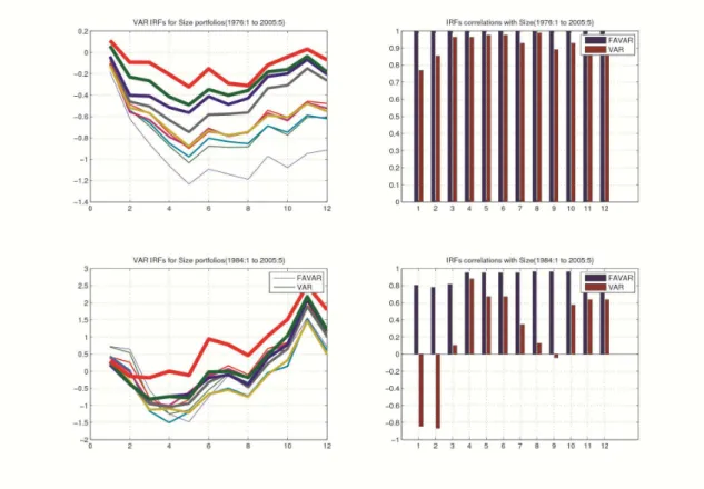
Even though the identified monetary shocks uncovered by the FAVAR approach are quite similar to the ones obtained with ordinary small scale VARs, should we expect similar dynamics? Figure 6 compares the impulse response functions of the ten size portfolios obtained by the two approaches following a 25 basis contractionary monetary shock. This picture shows that for this model setup(number of lags = 13 and sample ranging from 1976:1 to 2005:5), there is a small difference in the impulse responses functions. This small difference, however, is enough to destroy the perfect monotonicity in the responses of the ten size portfolios. This is illustrated in figure 7. The left pictures show the impulse response of all these portfolios in the same plot. As before, large caps are represented by thicker lines. The pictures on the right of figure 7 show the order correlation between these responses and market capitalization. We plot again in this same picture the order correlation obtained with the FAVAR approach for comparison. The bottom pictures show analogous results for the estimation using the subsample ranging from 1984:1 to 2005:1.
Figure 6: FAVAR x VAR impulse response functions for 10 size portfolios.
of stocks responses to a monetary shock. Although we do not report the results here, we observe a similar deterioration of the explanatory power of the other proxies for dependence on external finance. We believe that this happens due to the failure of the standard VARs in incorporating all relevant macroeconomic and financial information. This is where the FAVAR approach shows its full power. Indeed, to estimate the FAVAR dynamical system we use the entire data set that contains hundreds of time series. This could not be done with an ordinary VAR due to degrees-of-freedom problems. Indeed, most VARs in the related literature (e.g. Leeperet al. (1996) )do not use more than 20 variables. Given such limitation, a researcher has to make a somewhat arbitrary choice of the series to be used in the analysis. For example, it is known that a measure of ”economic activity” is important in most macroeconomic empirical studies. But what time series should be used to represent ”economic activity”? Gross domestic product? Gross national product? Unemployment? Industrial production? This situation is still more uncomfortable if we have to choose among several measures of ”price pressures”. The very existence a whole plethora of inflation indexes points out that maybe no single inflation index captures the notion of ”price pressures” in a dominant way. If we are forced to choose only one index to include in a model and discard the remaining ones due to degrees-of-freedom problems, we may be throwing away useful information. The FAVAR approach spares us of making this type of arbitrary choice by using the available data altogether.
5
Do the Fama-French Factors matter for monetary
pol-icy?
Figure 7: Impulse response functions and for size portfolios and their order correlation.
Yt =
Rt
M ktt−RFt
SM Bt
HM Lt
(3)
In which Rt is the Federal Funds Rate, M ktt is the market return, RFt is the one-month
t-bills(and therefore M ktt−RFt is the market excess return), SM Bt is the small minus big
index and HM Lt is the high minus low index. As we are adding 3 variables to our formerly 6
dimensional VAR, we set the number of extracted unobseved factors to 3, in order to keep the low dimensionality of the VAR and thus avoid degrees-of-freedom problems.
reasoning we used to explain the analogous figure in the last section, we conclude that even more weight is put on the stocks less impacted by the monetary shock. In short, what this picture points out is that by imposing the Fama-French Factors as observed components we may be explaining an even bigger difference in the response of big and small caps. If this intuition is right, than we would expect theSM B to be more severely hit by the shock in this specification. Moreover the gap between different size portfolios should widen. These very two predictions are confirmed in Figure 8 panels B and C, respectively.
Figure 8: Impulse response functions for the benchmark specification(left) and the specification with the Fama-French Factors as observable components(right).
5.1
Other specifications and robustness
To check the robustness of the results we stressed the model in various dimensions4
equation and the results once again remained robust. Finally, we did the same analysis using the subsample period of 1984:1 to 2005:5, and the qualitative results remained unchanged.
6
Conclusion
In this paper we investigated whether monetary policy shocks affect the cross-section of stock returns. To that end, we used a macro factor-augmented VAR. This technology allowed us to use hundreds of macroeconomic and financial time series that in principle could be useful to identify monetary policy shocks. This virtually eliminates the problem of the small scope of the informational set that is typical in small scale VARs. Furthermore with the FAVAR approach we could measure the monetary shock impact on several equity portfolios and indexes within a single empirical framework.
References
Ben S. Bernanke and Alan S. Blinder. The federal funds rate and the channels of monetary transmission. The American Economic Review, 82(4):pp. 901–921, 1992.
Ben S. Bernanke and Kenneth N. Kuttner. What explains the stock market’s reaction to federal reserve policy? The Journal of Finance, 60(3):pp. 1221–1257, 2005.
Ben S. Bernanke, Jean Boivin, and Piotr Eliasz. Measuring the effects of monetary policy: A factor-augmented vector autoregressive (favar) approach. The Quarterly Journal of Eco-nomics, 120(1):pp. 387–422, 2005.
Jean Boivin, Marc P. Giannoni, and Ilian Mihov. Sticky prices and monetary policy: Evidence from disaggregated us data. The American Economic Review, 99(1):pp. 350–384, 2009. Mark Gertler and Simon Gilchrist. Monetary policy, business cycles, and the behavior of small
manufacturing firms. The Quarterly Journal of Economics, 109(2):pp. 309–340, 1994. Oliver Hart and John Moore. Default and renegotiation: A dynamic model of debt. The
Quarterly Journal of Economics, 113(1):pp. 1–41, 1998.
Eric M. Leeper, Christopher A. Sims, Tao Zha, Robert E. Hall, and Ben S. Bernanke. What does monetary policy do? Brookings Papers on Economic Activity, 1996(2):pp. 1–78, 1996. Raghuram G. Rajan and Luigi Zingales. Financial dependence and growth. The American
Economic Review, 88(3):pp. 559–586, 1998.
Glenn D. Rudebusch. Do measures of monetary policy in a var make sense? a reply to christo-pher a. sims. International Economic Review, 39(4):pp. 943–948, 1998.
James H. Stock and Mark W. Watson. Forecasting using principal components from a large number of predictors.Journal of the American Statistical Association, 97(460):pp. 1167–1179, 2002.