Março de 2015
Working
Paper
380
Dynamic coordination among
heterogeneous agents
• •
Os artigos dos Textos para Discussão da Escola de Economia de São Paulo da Fundação Getulio Vargas são de inteira responsabilidade dos autores e não refletem necessariamente a opinião da
FGV-EESP. É permitida a reprodução total ou parcial dos artigos, desde que creditada a fonte.
Escola de Economia de São Paulo da Fundação Getulio Vargas FGV-EESP
Dynamic coordination among heterogeneous agents
∗Bernardo Guimaraes† Ana Elisa Pereira‡
March 2015
Abstract
We study a dynamic model of coordination with timing frictions and payoff heterogeneity. There
is a unique equilibrium, characterized by thresholds that determine the choices of each type of agent.
We characterize equilibrium for the limiting cases of vanishing timing frictions and vanishing shocks to
fundamentals. A lot of conformity emerges: despite payoff heterogeneity, agents’ equilibrium thresholds
partially coincide as long as there exists a set of beliefs that would make this coincidence possible – though
they never fully coincide. In case of vanishing frictions, the economy behaves almost as if all agents were
equal to an average type. Conformity is not inefficient. The efficient solution would have agents following
others even more often and giving less importance to the fundamental.
Keywords: coordination, conformity, timing frictions, heterogeneous agents, dynamic games.
Jel Classification: C73, D84.
1
Introduction
Profitability of investment decisions depends on future demand for a firm’s good, which depends on whether other firms will be investing as well but also on idiosyncratic factors that affect demand for a particular product. In a problem of debt roll-over, both coordination motives and an individual’s appetite for risk have to be considered. When deciding between Facebook and Google+, a consumer will take into account what others have been choosing but also her own tastes. Similarly, adopting a new technology may not be the best decision if others in the production chain will keep working with an old technology but heterogeneity in agents’ productivity might also play an important role in this decision. In all these settings, both payoff complementarities and idiosyncratic features of preferences or technologies are important for an agent’s choice.
∗We thank Luis Araujo, Braz Camargo, Itay Goldstein, Caio Machado, Daniel Monte, Jakub Steiner and seminar participants at CERGE-EI, LAMES 2014 (Sao Paulo), Wharton and the Sao Paulo School of Economics – FGV. Bernardo Guimaraes gratefully acknowledges financial support from CNPq. Ana Elisa Pereira gratefully acknowledges financial support from FAPESP.
†Sao Paulo School of Economics – FGV.
Strategic complementarities induce players to try to do the same thing. In a dynamic setting, that means following what others are doing and what they are likely to choose in the future. However, the idiosyncratic component of payoffs might push agents in different directions. This paper studies the interplay of complementarities and heterogeneity in payoffs in a dynamic setting.
In order to study this question we consider a dynamic environment with timing frictions as inFrankel and Pauzner(2000). Agents make a binary choice between two actions (say joining Facebook or not). Agents’ instantaneous utility flow depends on an exogenously moving fundamental (which captures the intrinsic quality of Facebook), on how many others are in the network and on idiosyncratic tastes. Agents get opportunities to revise their behavior (join or leave Facebook) according to a Poisson clock, which can be seen as an attention friction modeled in a reduced form way.
We first show there is a unique rationalizable equilibrium where agents of a given type play according to a threshold that depends on the total number of agents in a network and on the exogenous fundamental. We then obtain analytical results for the limiting cases of vanishing shocks and vanishing frictions, and provide an analytical characterization of the equilibrium thresholds in a tractable case with linear utility. Last, we solve the planner’s problem to understand the inefficiencies that arise in equilibrium and assess the effects of policies targeting distinct types.
Each type of agent joins the network if the exogenous fundamental (θ) is larger than a threshold that is a function of the fraction of agents in the network (n). In the tractable limiting cases, a lot of conformity arises. Different types will always play the same strategy for some values on n unless their preferences are so heterogeneous that there is no set of (arbitrary) beliefs that would induce them to play according to the same threshold. Agents’ choices are more similar for intermediate values ofn, when there is more heterogeneity in their behavior – and more dispersion of beliefs in a neighborhood around the threshold. In case of vanishing frictions, although agents play according to different strategies, the economy behaves almost as if all agents were identical and equal to an average type (again, unless agents’ preferences are so heterogeneous that no set of beliefs could induce conformity).
Dvorak alternative because everybody else is used to the QWERTY standard, even though the Dvorak keyboard is better in terms of its intrinsic quality.1 The planner would be even
more inclined towards QWERTY.
As an application, we consider a simple economy where investment generates positive ex-ternalities and study how subsidies to each type affect the equilibrium. For an economy in a state where nobody is investing, the most ‘productive’ agents are the ones who trigger a recovery. The model can be used to understand whether the government should target the most productive agents with investment subsidies in order to get investment going. Interest-ingly, in case of vanishing frictions, the distribution of subsidies is essentially irrelevant for agents’ decisions, as subsidies to less productive agents have a strong effect on the behavior of the more productive ones.
This paper builds on the model of Frankel and Pauzner (2000). They base their analysis on a model of sectorial choice (along the lines of Matsuyama (1991)), but their framework has been used to analyze location choices (Frankel and Pauzner (2002)), carry trades and speculation (Plantin and Shin (2006)), speculative attacks (Daniëls (2009)) and investment and business cycles (Frankel and Burdzy(2005),Guimaraes and Machado(2014)). The model of currency attacks in Guimaraes (2006) and the model of debt runs in He and Xiong(2012) employ similar timing frictions.
The paper is related to the literature on coordination in games with strategic comple-mentarities. With complete information and no shocks, these games might exhibit multiple self-fulfilling equilibria. Carlsson and Van Damme(1993),Morris and Shin(1998) andFrankel et al.(2003) have shown that a unique equilibrium arise in a static environment in which fun-damentals are not common knowledge and agents have idiosyncratic information about them (the so called global games). Frankel and Pauzner (2000) and Burdzy et al.(2001) show that a small amount of shocks in a dynamic model (with no private information) yields similar results. The relation between both literatures is discussed inMorris (2014).2 In a related
con-tribution,Herrendorf et al.(2000) show that if there is enough heterogeneity and a continuum of types, there is a unique equilibrium even in a dynamic setting with complete information. Applied work employing the global games methodology has often considered heterogeneous populations.3 Our results can be used in applied settings where dynamic coordination and
heterogeneity are important. The application developed in this paper is inspired by Sakovics and Steiner (2012) who consider a static coordination game played by a heterogeneous pop-ulation and study the effect of investment incentives for each type of agent. They conclude
1
SeeDavid(1985).
2See alsoMorris and Shin(2003).
3Examples include heterogeneity in roles (Goldstein(2005)); wealth (Goldstein and Pauzner(2004)), risk aversion and
the government should subsidize those who generate important externalities but are not im-portantly affected by others’s actions.
The paper is also related to literature on network externalities, in which strategic comple-mentarities arise from consumption externalities.4 Agents’ optimal choices typically depend
on what they expect others will do. However, most of this literature makes ad-hoc assump-tions on how agents coordinate.5 One important exception isArgenziano (2008). She studies
welfare in a model with differentiated networks in a static global-game model and highlights two sources of inefficiencies: agents give too much importance to their own idiosyncratic tastes and firms with the larger network charge a higher price. Both effects contribute to make the network “too balanced”. Our work complements her work by pointing out inefficiencies coming from the dynamic interaction among agents.6
The efficiency results here contrast with those in models with information externalities that generate herd behavior (e.g.,Bikhchandani et al.(1992)). In those models, agents follow others too much from a social point of view. Here, conformity of behavior arises because of preferences, not through learning, and they follow others too little.
2
The model
There is a continuum of infinitely-lived agents indexed by i ∈ [0,1]. Time is continuous and agents discount the future at rate ρ. There are two possible actions ai ∈ {0,1}, but
agents cannot switch from one to another at will. They receive chances to revise their actions according to a Poisson process with arrival rate δ, and stay committed to this choice until the arrival of another opportunity. This timing friction might represent an attention friction of consumers or firms, a machine break-up in an environment with a choice between two technologies or maturity of debt in a model of debt runs.
The flow payoff an agent gets from either action depends on fundamentals, on her idiosyn-cratic preferences and on the actions of others (there are strategic complementarities). Let n
be the proportion of agents choosing action 1. Strategic complementarities can arise owing to either one-sided externalities or two-sided externalities: either the payoff of choosing action 0 is independent of the amount of agents making the same choice, but the payoff of choosing 1 is increasing inn (as in Matsuyama (1991)); or both actions become more appealing the larger is the proportion of agents taking them (as in Argenziano (2008)); or flow-payoffs from both actions can be increasing in n, but the difference in payoffs is also monotonically increasing
4This literature has started withKatz and Shapiro(1985) andKatz and Shapiro(1986). SeeShy(2011) for a survey. 5For instance,Katz and Shapiro(1986) assume that whenever there are multiple equilibria in the model, agents manage to
coordinate their decisions in order to achieve the Pareto-superior outcome.
inn (as in Guimaraes and Machado (2014)).
We denote agent i’s relative flow-payoff of choosing action 1 by πq(i)(θ, n), where θ ∈ R
denotes the fundamentals of the economy, n ≡ ´1
0 aidi is the fraction of agents currently
committed to action 1 andq(i)∈ {1, ..., Q}is agenti’s type. All functionsπq(.) are continuous
and strictly increasing in both arguments. If we let αq denote the mass of type-q agents in
the population and nq the proportion of type-q agents currently playing 1, n can be written
as n=PQq=1αqnq.
An agent who receives a chance to revise her choice at time τ will choose ai = 1 whenever
E ˆ ∞
τ
e−(ρ+δ)(t−τ)πq(i)(θt, nt)dt≥0
and ai = 0 otherwise. The expected discounted payoff takes into account only the states
in which the agent believes she will still be committed to her action (e−δ(t−τ) expresses the
probability of not receiving a revising opportunity between τ and t).
We further assume that payoff functions πq(.) are such that there are dominance regions
for all types of agents. For each type, there is a region in theR×[0,1] space where choosing action 0 is a dominant action, and a region in which choosing action 1 is a dominant action. In other words, for any given initial n, there is a sufficiently low level of fundamentals at which an agent prefers to play 0 even if she expects all others to play 1 when they get a chance to revise their actions, and there is a sufficiently high level of fundamentals such that it is preferable to play 1 even if no one else is expected to choose so in the future.
LetPq be the boundary of the upper dominance region of a type-q agent, i.e., the curve on
which such agent is indifferent between the two actions if she believes everyone after her will choose 0 (P stands forpessimisticabout the proportion of agents playing 1 in the future). This boundary is downward sloping: sinceπq(θ, n) is increasing inθand n, a highern today means
that the value of θ needed to make agents indifferent between the two actions is smaller. At the other extreme, let Oq be the boundary of the lower dominance region for a type-q player,
that is, the curve on which this type of agent is indifferent between the two actions under the belief that everyone will choose 1 when they get the chance (O stands for optimistic). This curve is also downward sloping.
2.1 Unique equilibrium
multi-Figure 1: Dominance regions: an example
θ n= 1
n= 0
O1
O3 P3 O2 P2 P1
plicity.7
However, when there are shocks to θ, the equilibrium is unique for any amount of hetero-geneity. Proposition1presents this result. The following lemma is key for the demonstration. It states that the dynamics of n depends on (θt, nt) but not on each nq,t, q∈ {1, ..., Q} (for a
given nt).
Lemma 1. For any given strategy profile, the dynamics of ndepends only on the state(θt, nt).
Proof. Fix a strategy profile nsq(i)
o
q∈{1,...,Q}. Denote by It the set of types playing 1 at time
t. Notice that the path of nq is given by the following differential equation:
∂nq,t ∂t =
δ(1−nq,t) ifq∈ It
−δnq,t ifq /∈ It
(1)
Equation 1means that a type-qagent whose strategy prescribes playing 1 and is currently playing 0 will switch to action 1 when she receives an opportunity to revise her choice (there are 1−nq,t such agents). Likewise, every type-q agent whose strategy prescribes playing 0
and who has previously chosen 1 will switch to action 0 at the first opportunity. Using the fact that n=PQq=1αqnq,t, we have that ∂n∂tt is given by:
∂nt ∂t =
Q X
q=1
αq ∂nq,t
∂t !
= X
q∈It
αqδ(1−nq,t) + X
q /∈It
αq(−δnq,t)
=δ
X
q∈It αq−
Q X
q=1
αqnq,t
7Herrendorf et al.(2000) shows that in a similar environment with no shocks and a continuum of types, multiplicity is ruled
=⇒ ∂nt
∂t =δ
X
q∈It
αq−nt
Lemma1allows us to deal with this problem in a two-dimensional space: agents only need to look at the fundamentals (θt) and at the aggregate mass of agents currently committed to
action 1 in order to understand the dynamics of the system. One could expect this dynamics to depend on the proportion of each type of agent currently on each option, but due to the assumption of a Poisson process for the arrival of opportunities to switch actions, that is not true. It suffices to know the aggregate nt and each type’s strategy to compute∂nt/∂t.
Proposition 1. Suppose θ follows a Brownian motion with drift µ and variance σ2 > 0.
There is a unique equilibrium characterized by downward sloping thresholds Z∗
q
q∈{1,...,Q} in
the R×[0,1] space, such that
ai,t =
1 if θt> Zq∗(i)(nt)
0 if θt< Zq∗(i)(nt)
That is, each agent i called upon acting at time t plays 1 when to the right and 0 when to the left of Z∗
q(i).
Proof. See AppendixB.1.
The proof of equilibrium uniqueness employs a strategy of iterative elimination of strictly dominated strategies, starting from the dominance regions. Even if these regions are very remote, making it unlikely that the fundamentals will reach one of them before an agent receives another chance to revise her action, the existence of such regions triggers an iterative contagion effect until there is a single rationalizable strategy left (for each type of agent). The basic intuition is as follows: an agent at any point on the boundary of her upper dominance region is indifferent between actions 0 or 1 under the assumption that, at all future dates, all other agents will choose 0. But once shocks to fundamentals are introduced, she knows there is a positive probability that fundamentals will reach regions in which it is dominant for some agents to play 1 (while she is still committed to her choice).8 Thus, she cannot
hold the belief that others will play 0 under any circumstances. The most pessimistic belief she can hold is that agents will play 0 whenever it is not strictly dominated to do so, and under this new (a bit more optimistic) belief, there is another (smaller) level of fundamentals that makes such agent indifferent between the two actions. Extending this reasoning to all
following rounds and employing an analogous procedure starting from the lower dominance regions yields a unique rationalizable equilibrium. An interesting aspect of this result – which was demonstrated byFrankel and Pauzner(2000) for the case of identical individuals – is that uniqueness of equilibrium can be achieved even with vanishing shocks to fundamentals (that is, in the limit as µ, σ → 0). Multiplicity of equilibrium in this environment do not survive the introduction of the smallest amount of shocks.
The unique equilibrium is characterized by thresholds for each type of agent, to the right of which these agents play 1, and to the left of which they play 0. Depending on the initial value of n, these strategies imply an upward or downward path for nt. Figure 2 below exemplifies
the dynamics around the equilibrium for a case with three types of agents. ∂nt/∂tis computed
as in Lemma 1.
Figure 2: Dynamics (Q= 3)
θ n= 1
n= 0
˙
n=δ(1−n)
˙
n=−δn
˙
n=δ(α1−n)
α1+α2 Z∗
1 Z2∗ Z
∗ 3
α1
˙
n=δ(α1+α2−n)
3
Limiting cases
We now restrict our attention to situations with two types, Q= 2, and analyze two limiting cases: vanishing shocks to fundamentals and vanishing timing frictions. Assumeq(i) = q∀i∈
[0, α] and q(i) = q ∀i ∈ (α,1], i.e., there is a mass α of type-q agents in the economy and a mass 1−α of type-q agents. Denote their payoff functions, respectively, by π(θ, n) and
π(θ, n). We assume that for any pair (θ, n), π(θ, n) > π(θ, n), that is, type-q agents have a higher relative instantaneous payoff of choosing action 1 in every state.
The next lemma, based on Burdzy et al. (1998), characterizes agents’ beliefs on the equi-librium threshold and is key for the results of the paper.
Lemma 2. Suppose agents play according to distinct thresholdsZ(n)< Z(n)for allnin some interval (n1, n2). Consider a point (θ, n) with θ=Z∗
i(n) for some i∈[0,1] and n ∈(n1, n2).
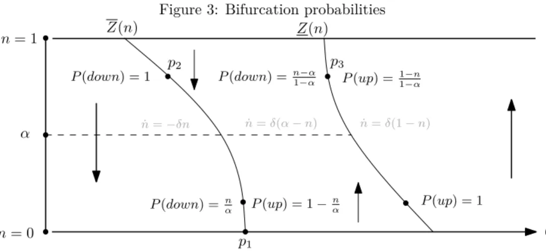
Figure 3: Bifurcation probabilities
θ n= 1
n= 0
α
Z(n) Z(n)
P(down) = 1
P(up) = 1
P(down) =n
α P(up) = 1− n α
P(down) = n−α
1−α P(up) = 1−n 1−α
˙
n=δ(α−n) n˙=δ(1−n)
˙
n=−δn
p1
p2 p3
Moreover, the probabilities of an upward or a downward bifurcation are computed as follows: (i) Consider a point (θ, n) with θ=Z(n).
P(up) =
0 if n ≥α
1− n
α if n < α
and P(down) = 1−P(up).
(ii) Consider a point (θ, n) with θ =Z(n).
P(up) =
1−n
1−α if n > α
1 if n ≤α
and P(down) = 1−P(up). Proof. See AppendixB.2.
Figure3shows the dynamics around the two types’ thresholds in case they do not intersect (computed as in the proof of Lemma 1) and the implied bifurcation probabilities along the thresholds (computed as in Lemma 2). The idea behind Lemma 2 is that, considering an initial point exactly on an agent’s threshold, the probability of the system going up or down depends on the speed of increase or decrease of n at each side of the threshold. Intuitively, once the economy has headed off in one direction, it does not revert to Z∗
i, since thresholds
are downward sloping and shocks to fundamentals are small, but will it start going up or down? That depends on the realization of the Brownian motion in a tiny space of time and on the speed of decrease and increase ofn at each side of the threshold that pull the economy away from the (downward sloping) threshold.
revising her action when the economy is at p1 in Figure 3. As n = 0, a small negative shock
pushing θ slightly to the left will make no difference (n cannot decrease anymore), while a small positive shock to θ will lead high type agents to choose action 1, so agents believe that
n will increase with probability one. An agent at point p2 holds the opposite belief but for a
different reason: both to the left and to the right of Z, n is decreasing, so the agent assigns probability one tonheading towards zero. Last, look at pointp3in Figure3. A small negative
shock to θ means that all high-type agents who get the chance will play 1, but all low-types will play 0. Since there are more agents currently committed to 1 than agents willing to choose 1 (because n > α), n decreases in that region at a rate δ(n−α). A small positive shock, though, would make every agent willing to switch to action 1, hence n would increase at rate δ(1−n). This dynamics implies that at p3, the probability of the system bifurcating
up is proportional to the relative rate at which it goes up: δ(1−δn(1−)+δn()n−α) = 1−n
1−α.
3.1 Vanishing shocks
Consider the limiting case in which shocks to fundamentals vanish, that is,µ→0 andσ →0. LetZ(n) andZ(n) denote the two types’ equilibrium thresholds. The equilibrium properties depend on the degree of payoff heterogeneity.
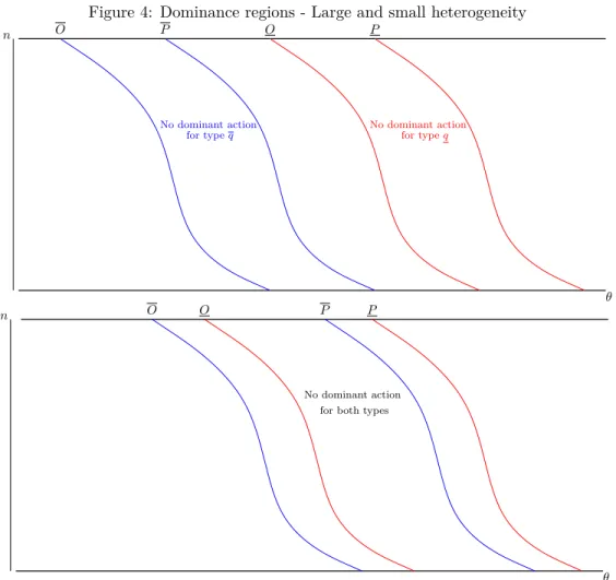
The relative position of the dominance regions for the two types of agents on theR×[0,1] space reflects the degree of heterogeneity in their payoff functions. For a sufficiently large degree of heterogeneity, we have thatP(n)< O(n)∀n: a high-type agent that holds the worst possible belief concerning future choices of others demands a smaller value of the fundamental to be indifferent between the two actions than a low-type agent under the most optimistic belief. This implies there is no region in the state space in which neither type has a dominant action. On the other hand, if heterogeneity is not too large, dominance regions can be such that O(n)< P(n)∀n, so there is a region in which neither action is dominant for both types of agents. Figure4 exemplifies those two cases.
In the case of vanishing shocks, the upper dominance region boundary of a high-type agent can be computed as:
ˆ ∞
0
e−(ρ+δ)tπ(P , n↓t)dt= 0, (2)
where n↓t =n0e−δt. The lower dominance region boundary of a low-type agent is given by
ˆ ∞
0
e−(ρ+δ)tπ(O, n↑t)dt= 0, (3)
Figure 4: Dominance regions - Large and small heterogeneity
n
θ
O P O P
No dominant action
for typeq No dominant actionfor typeq
n
θ
O O P P
No dominant action for both types
Expressions for the equilibrium thresholds are provided in Appendix A.1. Proposition 2
shows the main equilibrium properties for the case of vanishing shocks.
Proposition 2. Suppose there are two types of agents in the economy, q and q, with payoff functions given by π(θ, n) and π(θ, n), respectively, with π(.) > π(.) ∀(θ, n). In the limit as
µ, σ →0, in the unique rationalizable equilibrium:
(i) if O(n)> P(n)∀n, thenZ(n)< Z(n)∀n, so different types’ thresholds do not intersect; (ii) if O(n)< P(n)∀n, then Z(n) = Z(n) for alln in an interval containingα. Moreover, there are neighborhoods around 0 and 1 in which Z(n)< Z(n).
Proof. See AppendixB.3.
strictly dominated strategy.
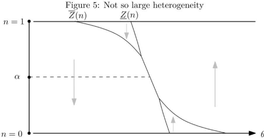
The second part of Proposition 2 brings a surprising result: there is some conformity in agents’ behavior as long as heterogeneity is not large enough to make it impossible for agents to play according to the same threshold for any (arbitrary) set of beliefs. Proposition2also states that different players will choose according to the same threshold for an intermediate range ofn. Their thresholds will never fully coincide though: for extreme values ofn, heterogeneity beats coordination and each type has a distinct threshold. Figure5 exemplifies this result.
Figure 5: Not so large heterogeneity
θ n= 1
n= 0
α
Z(n) Z(n)
In order to understand the result in Proposition 2, suppose agents play according to dif-ferent thresholds as in Figure 3. For n =α, an agent at the lower threshold (the one at the left) holds the most pessimistic beliefs, n will surely decrease from then on. That is because all low-type agents will be choosing 0, and at n = α they are just enough to determine the path of the economy. Hence an agent will not choose action 1 unless it is dominant to do so. Conversely, an agent at the higher threshold (the one at the right) holds the most optimistic beliefs for exactly the same reason: high-type agents are choosing 1 and at n = α they are just enough to drive the economy up. Hence an agent will not choose 0 unless it is dominant to do so.
This reasoning implies that an equilibrium with two distinct thresholds at n=α requires (i) high-type agents being indifferent between either choice for some ˜θ holding the most pessimistic beliefs; and (ii) low-type agents being indifferent between either choice for some
θ >θ˜holding the most optimistic beliefs. This can only happen in case of very large payoff heterogeneity. If that is not the case, owing to the large dispersion in beliefs offsetting idiosyncratic payoffs, both thresholds will coincide at n=α.
difference in beliefs. Hence even a small difference in preferences leads to the existence of two distinct thresholds.
In sum, for intermediate values ofn, there is huge heterogeneity in expectations about the path of n around the equilibrium threshold, which makes payoff heterogeneity less relevant. In contrast, for extreme values of n, there is less uncertainty about the path of n around the equilibrium thresholds and hence heterogeneity in preference matters for agents’ optimal choice.
3.2 Vanishing frictions
We now consider the limiting case of δ → ∞ so that agents receive very frequent opportu-nities to revise their actions. Expressions for equilibrium thresholds under a general payoff function and vanishing frictions are provided in Appendix A.2. Proposition 3 emphasizes some properties of the equilibrium when distinct types’ flow payoffs differ by a constant.
Proposition 3. Let π(θ, n) = π(θ, n) +ε and π(θ, n) = π(θ, n) +ε, ε > ε. Define εˆ ≡
αε+ (1−α)ε andz∗, z∗ andzˆ∗ as satisfying ´α
0 π(z∗, n)dn=−αε, ´1
απ(z∗, n)dn=−(1−α)ε
and ´1 0 π(ˆz
∗, n)dn=−εˆ, respectively. In the limit as δ→ ∞:
(i) ifO(n)> P(n)∀n, the state space is divided in three regions: wheneverθt > z∗, nt≈1;
whenever z∗ < θ
t < z∗, nt ≈α and whenever θt< z∗, nt≈0.
(ii) if O(n)≤P(n)∀n, the vertical line zˆ∗ divides the state space in two regions: whenever
θt>zˆ∗, nt ≈1 and whenever θt <zˆ∗, nt ≈0.
Proof. See AppendixB.4.
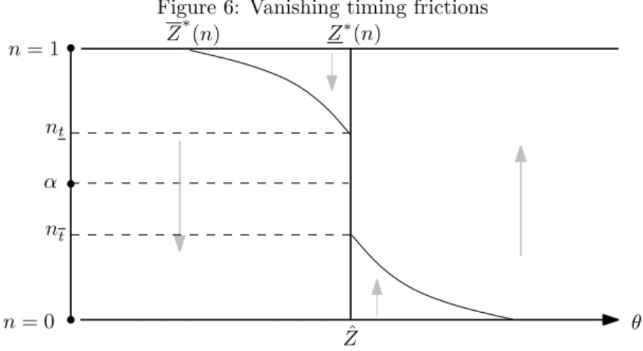
Proposition 3 states that in case of very large heterogeneity, at a given point in time, (almost) all agents of a given type will be playing the same action but different types might be playing different actions. The bounds of the region where behavior is heterogeneous (the switching point for each group) are determined by the value ofθsuch that, at n=α: (i) high types with pessimistic beliefs are indifferent between either action; and (ii) low types with optimistic beliefs are indifferent between either action.
When heterogeneity is not so large, in the limiting case of vanishing frictions, the economy behaves as if agents were identical and had an intermediate preference parameter ˆε. Although agents’ strategies differ, whenever fundamentals cross the vertical division line, all agents of a certain type immediately switch actions, leading the opposite type to consider it profitable to switch actions as well. Since chances to switch arrive at a very large rate, the dynamics of the economy is basically the same as if agents were identical with preferences given by ˆ
the limiting case of vanishing frictions, two networks can only coexist if there is no set of (arbitrary) beliefs that would lead different agents to play according to the same threshold.
Figure 6 depicts the equilibrium in case of not so large heterogeneity. Note that agents’ strategies differ for values ofn close to 0 and 1. As explained before, that is because for high and low values of n, beliefs at both thresholds are not so different, so payoff heterogeneity matters. This intuition is not affected when δ is large – agents at n = 0 at the right of ˆz∗
know n will be moving up fast, but also that they will quickly get another chance to choose.
Figure 6: Vanishing timing frictions
θ n= 1
n= 0
α
Z∗(n) Z∗
(n)
ˆ
Z nt
nt
4
Linear payoff function
We now present a linear example that provides intuition on the forces at play and helps us to understand the relative effects of payoff heterogeneity and complementarities in preferences. Let the relative flow-payoff of action 1 in comparison to action 0 be given by:
πi(θt, nt) = θt+γnt+εi
with
εi =
ε ∀i∈[0, α]
ε ∀i∈(α,1],
that is, there are two types of agents: a proportion α with preference parameter ε and a proportion 1−α with preference parameter ε,ε > ε.
4.1 Vanishing shocks
Consider again the case ofµ, σ →0. First, we compute the two dominance regions’ boundaries that can be used to measure the degree of heterogeneity in agents’ payoffs. Substituting our linear payoff function in equations (2) and (3) and solving the integrals yields the upper dominance region boundary of a high-type agent:
P(n0) = −ε−
γ(ρ+δ)
ρ+ 2δ n0, (4)
and the lower dominance region boundary of a low-type agent:
O(n0) =−ε−
γδ ρ+ 2δ −
γ(ρ+δ)
ρ+ 2δ n0. (5)
Large heterogeneity
The condition ensuring that P(n0)< O(n0)∀n0 is equivalent to
ε−ε > γδ
ρ+ 2δ. (6)
If the difference between idiosyncratic preference parameters is large enough in comparison to the importance of strategic complementarities (γ), the curve on which a high-type agent with pessimistic beliefs about n is indifferent between 0 and 1 is located to the left of the curve on which a low-type agent with optimistic beliefs is indifferent between the two actions. The intersection between the region in which neither action is dominant for a high-type agent and the region with no dominant action for a low-type agent is empty (as in the top picture of Figure4).
If condition (6) holds, then there is no set of beliefs that could induce different agents to play according to the same strategy for any value of n0. Hence, whenever this condition is
satisfied, the equilibrium in the limit asµ, σ → 0 will be such that type-ε and type-ε agents play according to thresholds that do not intersect, as stated in Proposition 2.
How can we analytically compute the thresholds in this case?9 First note that for alln ≥α
the high-type threshold coincides with the high-type upper dominance region. The belief a type-ε agent holds in equilibrium at some point (θ, n) with n ≥ α is that n will fall at the maximum rate with probability one (see Figure 3). Under the most pessimistic belief, this agent is indifferent between the two actions. Thus, type-ε agents’ threshold above α is a function Z(n0) = P(n0), and thus satisfies equation (4). Likewise, for all n ≤α the low-type
9
threshold must coincide with the low-type lower dominance region (in which agents hold the most optimistic belief), so forn0 ≤α, O(n0) is given by equation (5).
What about the high-type threshold belowαand the low-type threshold aboveα? Suppose, for now, that heterogeneity is large enough so that the following inequality holds:
ε−ε > γ(δ+ρα)
ρ+ 2δ . (7)
This condition ensures the equilibrium is such that Z(0) < Z(α), so that if the economy is initially at some point on Z(n0) with n0 < α, it will never reach n = 1: it will either go
down towards n = 0 or up towards n = α. In other words, the system will never cross the other type’s threshold. Graphically, it means that p1 is to the left ofp2 in Figure 7. We can
then compute the high-type equilibrium threshold below α as follows:
(α−n0)
α
| {z }
P(up)
ˆ ∞
0
e−(ρ+δ)tπ(Z, α−(α−n0)e−δt
| {z }
ntgrowing towardsα
)dt+ n0
α |{z} P(down)
ˆ ∞
0
e−(ρ+δ)tπ(Z, n0e−δt
| {z } ntfalling
)dt= 0.
The first term of the sum is the probability of an upward bifurcation times the discounted relative payoff of action 1 when the agent expects nt to grow until it approaches α. The
second term is the probability of a downward bifurcation times the discounted payoff when the agent expectsntto decrease towards zero. Substituting our linear functional form forπ(.)
and solving the integrals, we have that, whenever (7) holds, Z is given by
Z(n0) =
−ε− γρ(ρ+2+δδ)n0 if n0 ≥α
−ε− ραγδ+2δ −ρ+2γρδn0 if n0 < α
. (8)
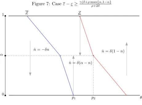
Analogous expressions for the low-type equilibrium threshold are derived in AppendixA.3. Figure 7depicts the equilibrium in case ε−ε > γ(δ+ρmax{ρ+2δα,1−α}, that is, the case in which if the economy starts at one threshold, it will never cross the other one. 10
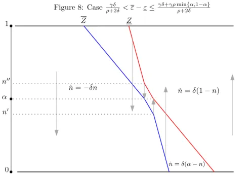
Now, suppose heterogeneity is still large so that P is to the left of O, but not as large as before. Specifically, assume
γδ
ρ+ 2δ < ε−ε≤
γ(δ+ρα)
ρ+ 2δ . (9)
Define n′ ≡ α − (ρ+2δ)(ε−ε)−γδ
γρ .
11 The threshold Z is still given by equation (8) for all
10
Figure 7: Caseε−ε≥ γ(δ+ρmaxρ+2{δα,1−α} 1 θ Z Z α 0 ˙
n=−δn n˙ =δ(1
−n)
˙
n=δ(α−n)
p1 p2
n0 ≥n′, but for all n0 < n′, it satisfies:
(α−n0)
α
| {z }
P(up) ˆ t 0
e−(ρ+δ)tπ(Z, α−(α−n0)e−δt
| {z }
ntgrowing towardsα
)dt+
ˆ ∞
t
e−(ρ+δ)tπ(Z,1−(1−n0)e−δ(t−t)
| {z }
ntgrowing towards 1
)dt n0 α |{z} P(down) ˆ ∞ 0
e−(ρ+δ)tπ(Z, n0e−δt
| {z } ntfalling
)dt = 0 (10)
where t is the time at which the system reaches the other type’s threshold, and it is given by t = −1
δln α−nt
α−n0, nt = Z
−1Z(n 0)
. This expression can be better understood with the aid of Figure 8. There is a range of n (n is sufficient low) such that a type-ε agent on her threshold knows that, if the system bifurcates up, it will cross the other type’s threshold at some point, and thereafter n will grow at a higher rate. Then, given this more optimistic belief, the increase in the level of fundamentals an agent demands to be indifferent between the two actions for a given decrease in n0 is smaller, i.e., the threshold is steeper.
Using the fact that Z(n) = O(n) for all n ≤ α and performing a change of variables in equation (10), we find that, whenever (9) holds, ∀n0 < n′,Z satisfies
(ρ+2δ)(Z+ε)+γρn0+γδα+γδ
(1−α)
α
1
α−n0
ρδ "
α+ (Z+ε)(ρ+ 2δ) +γδ
γ(ρ+δ)
#ρ+δδ
Figure 8: Case ρ+2γδδ < ε−ε≤γδ+γρminρ+2{δα,1−α}
1
θ
Z Z
α
0
˙
n=−δn n˙ =δ(1
−n)
˙
n=δ(α−n) n′
n′′
Not so large heterogeneity
Finally, consider the case in which P(n0)≥O(n0)∀n0, which is equivalent to
ε−ε≤ γδ
ρ+ 2δ. (12)
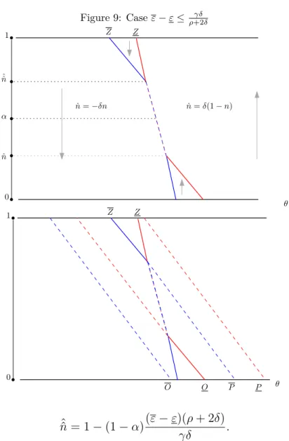
We know by Proposition 2that different-type agents’ strategies will coincide for some values of n, but never fully coincide. The equilibrium in this case is as depicted in Figure 9.
For all n0 ≤ nˆ, the type-ε threshold is identical to P(n0), and for all n0 ≥ nˆˆ, the type-ε
threshold is given by (11). Analogous equations describing the low-type threshold are provided in Appendix A.3.
In equilibrium, there is conformity in agents’ strategies for intermediate values of n as long as the condition in (12) holds. In most applications, ρ (time discount rate) is much smaller than δ (frequency of opportunities to revise behavior), so the expression in (12) can be approximated by ε−ε ≤ γ/2. In words, an equilibrium where agents play according to different thresholds requires payoff heterogeneity to be as important as an increase inn equal to half of the population. When (12) does not hold, there is no set of beliefs that would make conformity possible as P is to the left of O.
The bounds ˆn and ˆˆn in Figure 9 are given by
ˆ
n =α(ε−ε)(ρ+ 2δ)
Figure 9: Caseε−ε≤ρ+2γδδ
1
θ
Z Z
α
0
˙
n=−δn n˙ =δ(1−n) ˆˆ
n
ˆ n
1
θ
Z Z
0
O
O P P
ˆˆ
n= 1−(1−α)(ε−ε)(ρ+ 2δ)
γδ .
In case α= 1/2 and ρis much smaller than δ, we get ˆn ≈(ε−ε)/γ, thus ˆn is approximately equal to the increase in n that would compensate the idiosyncratic difference in payoffs.
Intuitively, the existence of type-εagents increases incentives for type-εto choose action 1, while the existence of type-εagents increases incentives for type-εto opt for 0. In consequence, agents behave in a more similar way. That is particularly true when n is in an intermediate range so that the path of the economy will be decided by the actions of both groups.
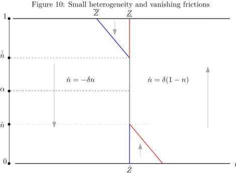
4.2 Vanishing frictions
Proposition6, or equivalently, take the limit asδ → ∞of all equilibrium thresholds computed in the previous subsection. The more interesting case is when O is to the left of P, which is equivalent to ε−ε ≤γ/2. Equilibrium is as in Figure 10. The line ˆZ divides the state space in two regions: whenever θt > Zˆ, nt ≈ 1, and whenever θt < Zˆ, nt ≈ 0. ˆZ coincides with
the equilibrium that would be played if there was just one type of agent in the economy with preference parameter ˆε≡αε+ (1−α)ε. ˆZ satisfies
ˆ
Z =−εˆ−γ/2.
Figure 10: Small heterogeneity and vanishing frictions
1
θ
Z Z
α
0
˙
n=−δn n˙ =δ(1−n)
ˆ ˆ
n
ˆ
n
ˆ
Z
The increase in nwhenθ crosses to the right of ˆZ atn≈0 is triggered by high-type agents choosing action 1, as low-type agents initially keep choosing 0. However, this difference in behavior will be very short lived. One implication of this result is that an increase in the mass of high-type agents (α) will affect the behavior of everyone in the economy (it will shift the threshold to the left) but there will be virtually no difference in the behavior of low-type and high-type agents.
5
The planner’s problem
We now solve the planner’s problem for the case of linear payoffs in order to analyze efficiency in this environment. All results in this section refer to the case of very small shocks,µ, σ →0. Agents face the choice between two actions, 0 and 1. The flow utility agent i derives from being committed to action 1 is given by u1
being at 0 is given byu0
i(θ0t, nt) =θ0t+ν0(1−nt)+ε0i. ntis the mass of agents currently playing
1, νj >0 is a parameter measuring the relative importance of strategic complementarities in
the choice ofj,θjt represents the fundamentals affecting the flow-payoff of playingj at timet,
and εji captures an idiosyncratic preference for actionj,j ∈ {0,1}.12 We will refer to 0 and 1
as networks, since the measure of agents playing each action generates externalities that can be thought of as network effects.
5.1 The case with ex-ante identical agents
In the case with ex-ante identical agents, we can setεji = 0 for j ∈ {0,1}. Hence the relative
payoff function can be written as
πi(θt, nt) =θt+γnt∀i,
where θt≡θt1−θt0−ν0 and γ ≡ν0+ν1.
The planner’s problem at time zero is to maximize the discounted sum of payoffs across agents, i.e.,
W =E ˆ ∞
t=0
e−ρthntut1+ (1−nt)u0t i
dt=
ˆ ∞
t=0
e−ρthnt
θt−ν0
+γn2tidt. (13)
At every point in time, the planner decides whether those with an opportunity to revise their actions will opt for 0 or 1. Action 1 is optimal if an infinitesimal increase inntpays off.
The effect on nt of an increase inn0 bydn0 is given bydnt =dn0e−δt since the initial increase
inn0 depreciates at a rateδ. From (13), the planner is indifferent between actions 0 and 1 if
E ˆ ∞
0
∂[e−ρt(n
t(θt−ν0) +γn2t)] ∂nt
dnt dn0
dt= 0,
which can be written as
E ˆ ∞
t=0
e(ρ+δ)thθ
t−ν0+ 2γnt i
dt= 0. (14)
This expression is very similar to the indifference condition in the decentralized equilibrium: an agent is indifferent between 0 and 1 when E´∞
t=0e
(ρ+δ)t[θ+γn
t]dt = 0. There are 2
differences: (i) the externality is more important for the planner (γis multiplied by 2) because the planner also takes into account the spillovers on others; and (ii) the planner might be more inclined towards one of the actions depending on whether we have one-sided or two-sided network externalities (which is captured by ν0 in the equation).
Mathematically, this problem is very similar to the one solved by agents in the decentralized equilibrium: at every timet, the planner chooses according to (14) and beliefs about the future path of n must be consistent with optimality at every point. Hence the planner’s problem is equivalent to a game played by agents with payoffs given in (14), so the planner would choose according to a downward sloping threshold. Proposition 4 relates the planner’s solution to the decentralized equilibrium.
Proposition 4. Suppose there is a single type of agent in the economy. The decentralized equilibrium prescribes playing 1 whenever θt > Z∗(nt) and 0 otherwise, where Z∗ is given by
Z∗(n) =− γδ
ρ+ 2δ − γρ
ρ+ 2δn. (15)
The planner’s solution prescribes playing 1 whenever θt> ZP(nt) and 0 otherwise, where ZP is given by
ZP(n) =ν0− 2γδ
ρ+ 2δ −
2γρ ρ+ 2δn.
In the case of symmetric network effects, that is, ν0 =ν1, the planner’s solution becomes
ZP(n) =− γδ
(ρ+ 2δ)+
γρ
2(ρ+ 2δ) − 2γρ
ρ+ 2δn. (16)
Proof. See AppendixB.5.
The weight given by the planner to the current size of the network in (16) is twice as large as the weight given by agents in the decentralized equilibrium in (15). Common sense might suggest that the planner would push the agents towards the best “fundamentals” (1 when θ
is high, 0 when θ is low) but the planner actually cares less about fundamentals than the agents. If agents prefer the QWERTY over the fundamentally more efficient Dvorak (i.e., if agents prefer to choose 0 even though action 1 would be the optimal choice if θ were the only relevant factor), the planner would be even more inclined to choose the fundamentally worse option. Intuitively, the planner takes into account the externality on others that agents fail to internalize, while the intrinsic quality of each good is fully taken into account by agents in the decentralized equilibrium.13
Figure 11 depicts the results in Proposition 4 when ν0 = ν1, so there is no difference in
terms of externalities. The planner rotates the threshold so that its slope is half of the slope of the threshold in a decentralized equilibrium, which means n is relatively more important for the planner.
13
Figure 11: Planner’s Problem: identical agents n= 1
θ n= 0
Z∗ ZP
1 2
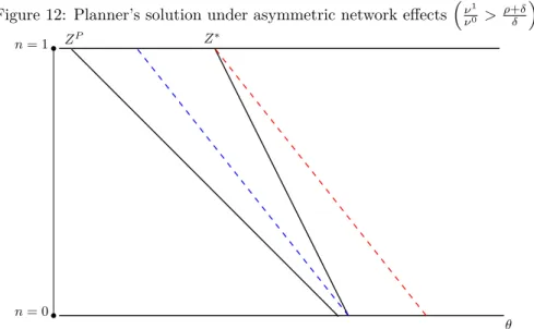
When the network effect is asymmetric, that is, ν0 6= ν1, the planner not only rotate
the threshold around n = 0.5, but it also shifts the threshold in order to enlarge the region in which agents choose the action that generates more externalities. Figure 12 depicts the planner’s solution whenν1/ν0 is larger then (ρ+δ)/δ.
Figure 12: Planner’s solution under asymmetric network effectsν1
ν0 >
ρ+δ δ
n= 1
θ n= 0
Z∗ ZP
When the externality in one network is large enough in comparison to the other, as in Figure 12, the planner’s threshold lies completely on the agents’ lower dominance region, so in the region between the lower dominance region boundary andZP, the planner prescribes a
strictly dominanted strategy to be played by everyone. To see why, consider for example the case in whichnis large. The planner takes into account that a lot of agents are stuck in action
1 (due to timing frictions) and they all would benefit from the network effects generated by an additional increase in n.
5.2 The case with two types of agents
In this section, we consider the planner’s problem in the case with two types of agents. Proposition 4 shows that differences between externalities from each network (ν0 and ν1)
only add a constant to the planner’s threshold, so we now focus on the case ν0 =ν1 =ν, for
simplicity of exposition. The planner’s problem in this case can be written as
maxEα
ˆ ∞
0
e−ρtnnt h
θt1+νnt+ε1 i
+ (1−nt) h
θt0+ν(1−nt) +ε0 io
dt
+ (1−α)
ˆ ∞
0
e−ρtnnt h
θt1 +νnt+ε1 i
+ (1−nt) h
θt0+ν(1−nt) +ε0 io
dt,
which is equivalent to
maxE ˆ ∞
0
e−ρt
nt
θt− γ
2 +γnt)
+αntε+ (1−α)ntε
dt,
where ε ≡ ε1 −ε0 and ε ≡ ε1 −ε0. Following the same reasoning as in the case of identical
agents, we find that the optimality conditions for the planner are given by
E ˆ ∞
0
e−(ρ+δ)t
θt+ε− γ
2 + 2γnt
dt= 0,
and
E ˆ ∞
0
e−(ρ+δ)t
θt+ε− γ
2 + 2γnt
dt= 0.
Proposition 7 in Appendix A.4 characterizes the planner’s solution analytically. Some of the results are illustrated in the figures below.
The planner’s solution has interesting properties. As before, its threshold is always flatter than in the decentralized equilibrium, meaning that the planner sacrifices gains stemming from good fundamentals in order to explore strategic complementarities (the planner is an enthusiast of QWERTY in this case as well). Moreover, the region in which the planner prescribes that the same strategy must be played by different types is always larger, showing that the planner cares less about idiosyncratic preferences as well.14 Figures13and 14depict
the planner’s solutions for different ranges of heterogeneity in comparison to the decentralized solution.
14InArgenziano(2008), the planner also gives a lower weight to idiosyncratic preferences but the dynamic (QWERTY) effect
Figure 13: Planner’s solution when γ(δ+ρmaxρ+2{α,δ(1−α)}) < ε−ε≤ρ2+2γδδ
1
θ
Z Z
α
0
ZP ZP
ˆ
nP
ˆ ˆ
nP
Figure 13 considers a case with large heterogeneity. In the decentralized equilibrium, for some values ofθ, two networks will coexist for long periods of time, with some agents choosing 1 and others going for 0. However, the efficient outcome would feature a single network (except for brief transition periods). The strategies prescribed by the planner imply that n would almost always be very close to 0 or 1.
In the example in Figure 14, heterogeneity is not so large and the equilibrium threshold of both types coincide for some values ofn. In this case, the range of values ofnfor which agents choose different actions is (exactly) twice as large as the analogous range for the planner.
Figure 14: Planner’s solution when ε−ε≤ γδ ρ+2δ
1
θ
Z Z
α
0
ZP ZP
ˆ ˆ
n
ˆ ˆ
nP
ˆ
nP
ˆ
6
Who matters in dynamic coordination problems?
We now consider the case where the planner would like agents to choose action 1 more often. For concreteness, suppose the choice agents face is between investing or not. Investment generates positive spillovers, so the payoff from investing depends positively on a fundamental (θ) and on the fraction of agents that have chosen to invest (n).15 Who matters in this dynamic
coordination problem?16
Consider the case where heterogeneity is not so large, as in Figure 9. If the economy is at a low-n state, the planner is mostly concerned with the high-type agents, since they are the ones who will trigger a switch to the regime with large n. Would the planner be particularly interested in subsidizing the high type then? In general, should the target of investment subsidies vary along the business cycle?
We briefly examine this question by studying the effect of a constant subsidy to agents, a flow amount ofs to each high-type agent and sto each low type conditional on them playing 1 (investing). Payoffs are linear and shocks are very small as in Section 4. Relative payoffs from investing are given by:
π(θt, nt) = θt+γnt+ε+s and π(θt, nt) = θt+γnt+ε+s.
Consider a situation in which n is close to 0 (few firms are investing) and subsidies are intended to trigger a switch to a high-n state. Using the expressions for the high- and low-type thresholds at low values of n given by (11) and (35), respectively, we have that:
∂Z ∂s =−
α
α+ (1−α)Ω and
∂Z ∂s =−
(1−α)Ω
α+ (1−α)Ω
where Ω = (α−n)−ρδ
α+ (Z+εγ)((ρρ+2+δδ))+γδ
ρ δ
<1 and
∂Z
∂s = 0 and ∂Z
∂s =−1.
Since there is a proportion α of high-type agents, paying 1/α units of subsidy to each high-type agent costs the same as paying 1/(1−α) units to each low type. Hence subsidies to high types have a stronger effect on their own threshold Z as long as Ω < 1, which is always true. In contrast, the threshold for low typesZ is importantly affected by subsidies to
15Guimaraes and Machado(2014) present a macroeconomic model where investment decisions are strategic complements in a
similar environment.
16
low-type agents but not at all by subsidies to high types.17 Intuitively, subsidies to low types
affect the beliefs of high types in a pivotal contingency, but subsidies to high types have no effect on beliefs of low types – at their equilibrium threshold, for low values of n, their beliefs are as optimistic as possible.
When n is small, shocks are very small and θ is at the left ofZ, we are mostly concerned with shifting Z to the left, because θ moves very slowly. Whenever the economy gets to the right of Z, high-types will start to invest, leading n to increase and soon the economy will cross the threshold for low types as well.18 Since Ω<1, direct subsidies to high types are the
best strategy to bring the economy closer to a recovery.
In contrast, when n is close to one, the best strategy to avoid an investment slump would be to subsidize the low types, who are the first ones to stop investing when fundamentals deteriorate. Preventing that is enough to keep high types willing to invest, without providing them with any direct incentives.
However, in many applications, it is reasonable to assume thatρ/δis small, that is, the rate at which agents discount the future is substantially smaller than the arrival rate of the Poisson process (which reflects, for example, the frequency at which a firm revises its investment and production decisions). In the limiting case of ρ/δ →0, we have that Ω→1, meaning that it does not matter who the government subsidizes. Interestingly, the indirect effect of s to low types on Z and the direct effect of s to high types on Z are exactly the same. Subsidizing low-type or high-type agents has exactly the same effect in the economy.
As shown in Proposition 3, the dynamics of this economy is well approximated by an economy with only one average type. Naturally, subsidies to either type have the same effect on the average type and hence will have the same effect on the equilibrium. Hence in case of very small frictions (very large values of δ), in order to get high types to invest and trigger a recovery, indirect subsidies to low types are as effective as direct subsidies to high types.
7
Final remarks
This paper shows that in a dynamic coordination model with timing frictions, heterogeneous agents will often play similar strategies. Agents predisposed to a certain action will be less willing to take it anticipating the behavior of agents less inclined to choose that action, and vice versa. That is particularly true when there is an intermediate number of people
17
The case with highnand subsidies aiming to avoid a decrease inn(prevent a recession as fundamentals start to deteriorate) is analogous. Subsidies to high types affect both thresholds, while subsidies to low types only affectZ, but the effect onZ is stronger if subsidies are channeled to low types.
18A shift of the low-type thresholdZto the left implies low types will choose to invest sooner after the recovery starts, but in
in a network, in which case there is more uncertainty about the path of the economy and coordination motives dominate idiosyncratic tastes. While the model is not intended to fit any particular application, the general lessons from the paper have implications for the policy debate.
As an example, the regulation of internet monopolies has been under discussion in the popular press and in the European Parliament.19 Network effects are key for internet
com-panies. Therefore, according to this paper, we should expect a lot of conformity in people’s choices, hence a lot of concentration, but occasional large (positive or negative) shifts in the market share of these firms – which is consistent with the stylized facts. Policy should then take into account that a social planner would be even more inclined towards concentration and conformity.
A
Expressions for the equilibrium thresholds
A.1 Vanishing shocks
Characterization of equilibrium in the limiting case of vanishing shocks is summarized in Proposition
5. Define Z0,Zα, Zα and Z1 as satisfying, respectively,
ˆ α
0
(α−n)ρδπ
Z0, n
dn= 0 (17)
ˆ 1
α
(1−n)ρδπ(Z
α, n)dn= 0 (18)
ˆ α
0
nρδπ
Zα, n
dn= 0 (19)
ˆ 1
α
(n−α)ρδπ(Z
1, n)dn= 0. (20)
Proposition 5. In the limiting case in which µ, σ→0, thresholds are computed as follows:
1. (Large heterogeneity) Case P(n)< O(n)∀n
(a) Type-q agents’ threshold:
i. If Z0 < Zα, then
• ∀n0 ≥α, Z(n0) =P(n0) and satisfies
ˆ n0
0
nρδπ
Z, ndn= 0; (21)
• ∀n0 < α, Z(n0) satisfies
ˆ n0
0
n
n0
ρ δ
π(Z, n)dn+
ˆ α
n0
α−n
α−n0
ρ δ
π(Z, n)dn= 0. (22)
ii. If Z0 ≥Zα, then
• ∀n0 ≥α, Z(n0) =P(n0) and satisfies (21);
• ∀n0 ∈(n′, α), Z(n0) satisfies (22);
• ∀n0 ≤n′,Z(n0) is the solution to the system
ˆ n0
0
n
n0
ρ δ
πZ, ndn+ ˆ nt
n0
α−n
α−n0
ρ δ
πZ, ndn
+
α−n t
1−nt
ρ+δ δ
ˆ 1
nt
1−n
α−n0
ρ δ
πZ, ndn= 0 (23)
ˆ 1
nt
(1−n)ρδπ(Z, n)dn= 0.
• n′ is the value satisfying Z(n′) =Z(α).
(b) Type-q agents’ threshold:
i. If Zα< Z1, then
• ∀n0 ≤α, Z(n0) =O(n0) and satisfies
ˆ 1
n0
(1−n)ρδπ(Z, n)dn= 0; (24)
• ∀n0 > α, Z(n0) satisfies
ˆ n0
α
n−α
n0−α
ρδ
π(Z, n)dn+ ˆ 1
n0
1−n
1−n0
ρδ
π(Z, n)dn= 0. (25)
ii. If Zα≥Z1, then
• ∀n0 ≤α , Z(n0) =O(n0) and satisfies (24);
• ∀n0 ∈(α, n′′), Z(n0) satisfies (25);
• ∀n0 ≥n′′, Z(n0) is the solution to the system
ˆ nt
0
n
n0−α ρ
δ nt−α
nt !ρ+δ
δ
π(Z, n)dn+ ˆ n0
nt
n−α
n0−α ρ
δ
π(Z, n)dn
+ ˆ 1
n0
1−n
1−n0
ρδ