LOW-COMPLEXITY ADAPTIVE FILTERING
LOW-COMPLEXITY ADAPTIVE FILTERING
Tese apresentada `a Escola Polit´ecnica da Universidade de S˜ao Paulo para obten¸c˜ao do T´ıtulo de Doutor em Engenharia El´etrica.
LOW-COMPLEXITY ADAPTIVE FILTERING
Tese apresentada `a Escola Polit´ecnica da Universidade de S˜ao Paulo para obten¸c˜ao do T´ıtulo de Doutor em Engenharia El´etrica.
´
Area de Concentra¸c˜ao:
Sistemas Eletrˆonicos
Orientador:
V´ıtor Heloiz Nascimento
I would like to thank my advisor, V´ıtor Heloiz Nascimento, for his inspirational and timely advice and constant encouragement over the last several years.
I also would like to thank Rodrigo de Lamare and Yury Zakharov for all the support during my PhD sandwich year at York.
Neste texto s˜ao propostos algoritmos de filtragem adaptativa de baixo custo computa-cional para o processamento de sinais lineares no sentido amplo e para beamforming.
Novas t´ecnicas de filtragem adaptativa com baixo custo computacional s˜ao desen-volvidas para o processamento de sinais lineares no sentido amplo, representados por n´umeros complexos ou por quaternions. Os algoritmos propostos evitam a redundˆancia de estat´ısticas de segunda ordem na matriz de autocorrela¸c˜ao, o que ´e obtido por meio da substitui¸c˜ao do vetor de dados original por um vetor de dados real contendo as mes-mas informa¸c˜oes. Dessa forma, evitam-se muitas opera¸c˜oes entre n´umeros complexos (ou entre quaternions), que s˜ao substitu´ıdas por opera¸c˜oes entre reais e n´umeros complexos (ou entre reais e quaternions), de menor custo computacional. An´alises na m´edia e na variˆancia para qualquer algoritmo de quaternions baseados na t´ecnicaleast-mean squares
(LMS) s˜ao desenvolvidas. Tamb´em ´e obtido o algoritmo de quaternions baseado no LMS e com vetor de entrada real de mais r´apida convergˆencia.
Uma nova vers˜ao est´avel e de baixo custo computacional do algoritmo recursive least squares (RLS) amplamente linear tamb´em ´e desenvolvida neste texto. A t´ecnica ´e mo-dificada para usar o m´etodo do dichotomous coordinate descent (DCD), resultando em uma abordagem de custo computacional linear em rela¸c˜ao ao comprimentoN do vetor de entrada (enquanto o algoritmo original possui custo computacional quadr´atico emN).
Para aplica¸c˜oes em beamforming, s˜ao desenvolvidas novas t´ecnicas baseadas no algo-ritmo adaptive re-weighting homotopy. As novas t´ecnicas s˜ao aplicadas para arrays em que o n´umero de fontes ´e menor do que o n´umero de sensores, tal que a matriz de auto-correla¸c˜ao se torna mal-condicionada. O algoritmo DCD ´e usado para obter uma redu¸c˜ao adicional do custo computacional.
In this text, low-cost adaptive filtering techniques are proposed for widely-linear pro-cessing and beamforming applications.
New reduced-complexity versions of widely-linear adaptive filters are proposed for complex and quaternion processing. The low-cost techniques avoid redundant second-order statistics in the autocorrelation matrix, which is obtained replacing the original widely-linear data vector by a real vector with the same information. Using this ap-proach, many complex-complex (or quaternion-quaternion) operations are substituted by less costly real-complex (or real-quaternion) computations in the algorithms. An analysis in the mean and in the variance is performed for quaternion-based techniques, suitable for any quaternion least-mean squares (LMS) algorithm. The fastest-converging widely-linear quaternion LMS algorithm with real-valued input is obtained.
For complex-valued processing, a low-cost and stable version of the widely-linear re-cursive least-squares (RLS) algorithm is also developed. The widely-linear RLS technique is modified to apply the dichotomous coordinate descent (DCD) method, which leads to an algorithm with computational complexity linear on the data vector length N (in opposition to the original WL technique, for which the complexity is quadratic inN).
New complex-valued techniques based on the adaptive re-weighting homotopy algo-rithm are developed for beamforming. The algoalgo-rithms are applied to sensor arrays in which the number of interferer sources is less than the number of sensors, so that the autocorrelation matrix is ill-conditioned. DCD iterations are applied to further reduce the computational complexity.
1 General description of an adaptive filter . . . p. 27
2 MSE comparison among linear and reduced-complexity
widely-linear algorithms, when the input is non-circular. . . p. 42
3 MSE comparison among linear and reduced-complexity
widely-linear algorithms, when the input is circular. . . p. 42
4 EMSE performance comparing QLMS, WL-QLMS, WL-QLMS, RC-WL-iQLMS, RC-WL-iQLMS, 4-Ch-LMS and the proposed second-order model, when the WL techniques are adjusted to achieve the same steady-state EMSE. The steady-state EMSE corresponds to -65 dB for RC-WL-QLMS
and RC-WL-iQLMS. – Average of 200 simulations. . . p. 74
5 MSD performance comparing QLMS, WL-QLMS, WL-QLMS, RC-WL-iQLMS, RC-WL-iQLMS, 4-Ch-LMS and the proposed second-order model, when the WL techniques are adjusted to achieve the same steady-state MSD. The steady-state MS corresponds to -47dB for RC-WL-QLMS and
RC-WL-iQLMS. – Average of 200 simulations. . . p. 75
6 EMSE performance comparing QLMS, WL-QLMS, WL-QLMS, RC-WL-iQLMS, RC-WL-iQLMS, 4-Ch-LMS and the proposed second-order model, when the WL techniques are adjusted to achieve the same steady-state MSD. The steady-state EMSE corresponds to -65 dB for RC-WL-QLMS
and RC-WL-iQLMS. – Average of 200 simulations. . . p. 76
7 MSD performance comparing QLMS, WL-QLMS, WL-QLMS, RC-WL-iQLMS, RC-WL-iQLMS, 4-Ch-LMS and the proposed second-order model, when the WL techniques are adjusted to achieve the same steady-state MSD. The steady-state MS corresponds to -47dB for RC-WL-QLMS and
RC-WL-iQLMS. – Average of 200 simulations. . . p. 77
8 First DCD iteration when w has only one element . . . p. 85
9 MSE comparison between the RC-WL-RLS, DCD-WL-RLS and SL-RLS
u b
11 MSE comparison between the RC-WL-RLS, DCD-WL-RLS and SL-RLS
algorithms, varying Mb and fixing Nu. Second scenario. . . p. 99
12 MSE comparison between the RC-WL-RLS, DCD-WL-RLS and SL-RLS
algorithms, varying Nu and fixing Mb. Second scenario. . . p. 99
13 MSE comparison between the RC-WL-RLS, DCD-WL-RLS and SL-RLS algorithms, when the coefficients change after 900 iterations. Nu = 8
and Mb = 2, 4, 8, 16. . . p. 100
14 MSE comparison between the RC-WL-RLS, DCD-WL-RLS and SL-RLS algorithms, when the coefficients change after 900 iterations. Mb = 16
and Nu = 1, 2, 4, 8. . . p. 100
15 Uniform linear array . . . p. 106
16 SINR performance when there are 5 faulty sensors. . . p. 130
17 Average number of homotopy iterations per snapshot when there are 5
faulty sensors. . . p. 130
18 SINR performance when there are 5 faulty sensors, but they are not
identified by the detector. . . p. 132
19 Average number of homotopy iterations per snapshot when there are 5
faulty sensors, but they are not identified by the detector. . . p. 132
20 SINR performance of the proposed techniques when the SNR varies. . . p. 133
21 Average number of homotopy iterations used by the proposed techniques
when the SNR varies. . . p. 134
22 Average number of homotopy iterations versus the number of sensors in
the array, when the number of interferers is constant. . . p. 135
23 Average number of homotopy iterations versus the number of sensors in the array, when the number of interferers grows linearly at the rate of
M/8. . . p. 137
24 Average number of homotopy iterations versus the number of sensors in
1 LMS algorithm . . . p. 28
2 RLS algorithm . . . p. 28
3 WL-LMS algorithm . . . p. 36
4 WL-RLS algorithm . . . p. 36
5 Computational complexity for SL-LMS, WL-LMS and RC-WL-LMS in
terms of real operations per iteration . . . p. 40
6 Computational complexity for SL-RLS, WL-RLS and RC-WL-RLS in
terms of real operations per iteration . . . p. 40
7 WL-QLMS algorithm . . . p. 54
8 WL-iQLMS algorithm . . . p. 55
9 RC-WL-iQLMS algorithm . . . p. 63
10 Computational complexity of the algorithms . . . p. 64
11 Step-sizes used in the simulations (µ= 10−3) . . . . p. 73
12 Real-valued cyclic-DCD algorithm . . . p. 88
13 Complex-valued cyclic-DCD algorithm . . . p. 89
14 Complex-valued leading-element DCD algorithm . . . p. 90
15 DCD-WL-RLS algorithm . . . p. 95
16 Computational complexity of the SL-RLS, WL-RLS, RC-WL-RLS and
DCD-WL-RLS per iteration . . . p. 95
17 C-ARH algorithm . . . p. 114
18 C-ARH algorithm applied to beamforming . . . p. 117
19 MC-C-ARH algorithm applied to beamforming . . . p. 119
20 It-C-ARH algorithm applied to beamforming . . . p. 121
23 Minimum computational complexity of C-ARH per snapshot (when the
total support size is K) . . . p. 126
24 Computational complexity per snapshot of the algorithms applied to
beamforming . . . p. 126
25 Total computational complexity of the algorithms using DCD iterations p. 127
26 Robust Capon beamformer . . . p. 140
27 Adaptive beamformer with variable loading . . . p. 141
1 4-Ch-LMS = Four channel least-mean squares algorithm
2 ARH = Adaptive re-weighting homotopy algorithm
3 BPSK = Binary phase-shift keying
4 C-ARH = Complex adaptive re-weighting homotopy algorithm
5 CH = Complex homotopy algorithm
6 DCD = Dichotomous coordinate descent algorithm
7 DCD-It-C-ARH = Iterative complex adaptive re-weighting homotopy algorithm us-ing dichotomous coordinate descent iterations
8 DCD-It-MC-C-ARH = Iterative multi-candidate complex adaptive re-weighting ho-motopy algorithm using dichotomous coordinate descent iterations
9 DCD-RLS = Dichotomous coordinate descent recursive least-squares algorithm
10 DCD-WL-RLS = Dichotomous coordinate descent widely-linear recursive least squares algorithm
11 DOA = Direction of arrival
12 EMSE = Excess mean-square error
13 FTF = Fast transversal filter
14 GLC = General-linear-combination-based robust Capon beamformer
15 It-C-ARH = Iterative complex adaptive re-weighting homotopy algorithm
16 It-MC-C-ARH = Iterative multi-candidate complex adaptive re-weighting homotopy algorithm
17 iQLMS = Quaternion least-mean squares algorithm obtained with the i-gradient
20 MC = Multi-candidate
21 MC-C-ARH = Multi-candidate complex adaptive re-weighting homotopy algorithm
22 MSD = Mean-square deviation
23 MSE = Mean-square error
24 MVDR = Minimum variance distortionless response
25 NLMS = Normalized least-mean squares algorithm
26 PAM = Pulse amplitude modulation
27 PSK = Phase-shift keying
28 QAM = Quadrature-amplitude modulation
29 QLMS = Quaternion least-mean squares algorithm
30 QRLS = Quaternion recursive least-squares algorithm
31 RC = Reduced-complexity
32 RCB = Robust Capon Beamformer
33 RC-WL-iQLMS = Reduced-complexity widely-linear quaternion least-mean squares algorithm obtained with the i-gradient
34 RC-WL-LMS = Reduced-complexity widely-linear least-mean squares algorithm
35 RC-WL-QLMS = Reduced-complexity widely-linear quaternion least-mean squares algorithm
36 RC-WL-RLS = Reduced-complexity widely-linear recursive least-squares algorithm
37 RLS = Recursive least squares
38 SINR = Signal-to-interference-plus-noise ratio
39 SL = Strictly-linear
40 SNR = Signal-to-noise ratio
43 WL = Widely-linear
44 WL-iQLMS = Widely-linear quaternion least-mean squares algorithm obtained with the i-gradient
45 WL-LMS = Widely-linear least-mean squares algorithm
46 WL-QLMS = Widely-linear quaternion least-mean squares algorithm
47 WL-QRLS = Widely-linear quaternion recursive least-squares algorithm
1 Introduction p. 17
1.1 Contributions of this work . . . p. 21
1.2 Organization of the text . . . p. 22
1.3 Notation . . . p. 22
Part I: LOW-COMPLEXITY WIDELY LINEAR ALGORITHMS p. 24
2 Low-complexity widely-linear adaptive algorithms for complex-valued
signals p. 25
2.1 Preliminaries . . . p. 26
2.1.1 Adaptive filtering . . . p. 27
2.1.2 Complex-valued widely linear estimation . . . p. 29
2.1.2.1 Circularity and second-order circularity . . . p. 33
2.1.2.2 Jointly second-order circular case . . . p. 34
2.1.2.3 Second-order circular regressor . . . p. 34
2.1.2.4 Real-valued desired signal (real d(n)) . . . p. 35
2.2 Reduced-complexity widely-linear adaptive filters . . . p. 36
2.2.1 Avoiding redundant information in the autocorrelation matrix . p. 37
2.2.2 Reduced-complexity widely linear LMS (RC-WL-LMS) . . . p. 38
2.2.3 Reduced-complexity widely linear RLS (RC-WL-RLS) . . . p. 39
2.3 Simulations . . . p. 41
2.4 Conclusions . . . p. 43
3 Reduced-complexity quaternion adaptive filters p. 44
3.1.2 Properties of Kronecker products . . . p. 47
3.2 Strictly-linear and widely-linear quaternion
estimation . . . p. 48
3.2.0.1 Q-properness . . . p. 50
3.2.0.2 Joint Q-properness . . . p. 51
3.2.0.3 Widely-linear estimation using real regressor vector . . p. 52
3.3 Quaternion gradients . . . p. 53
3.3.1 Case one: signals with correlation between at most two
quater-nion elements . . . p. 58
3.3.2 Case two: Widely-linear algorithms using real data vector . . . p. 60
3.3.2.1 The RC-WL-iQLMS algorithm . . . p. 61
3.3.2.2 Comparing the RC-WL-iQLMS with the 4-Ch-LMS
al-gorithm . . . p. 63
3.4 Analysis of QLMS-based algorithms . . . p. 64
3.4.1 Designing the step size to guarantee the convergence in the mean
of real-regressor vector techniques . . . p. 65
3.4.2 Mean-square analysis of QLMS-based algorithms . . . p. 65
3.4.3 Mean-square analysis of WL-QLMS algorithms with real input . p. 68
3.4.3.1 Choosing the step-size . . . p. 69
3.5 Simulations . . . p. 72
3.6 Conclusions . . . p. 77
Appendix A: Conditions to guarantee the positive semi-definiteness ofGextCext p. 79
Part II: LOW-COMPLEXITY TECHNIQUES USING THE DCD
AL-GORITHM p. 81
4 Low-complexity widely-linear adaptive filters using the DCD
4.2 The DCD-WL-RLS algorithm . . . p. 90
4.3 Simulations . . . p. 96
4.4 Conclusions . . . p. 101
5 Low-complex adaptive beamforming using the homotopy algorithm p. 103
5.1 System Model and Problem Statement . . . p. 105
5.1.1 Small number of interference sources . . . p. 107
5.1.1.1 Reducing the system of equations when there are faulty
sensors in the array . . . p. 108
5.2 Proposed complex homotopy algorithms . . . p. 109
5.2.1 The Complex Adaptive Re-Weighting Homotopy
Algorithm . . . p. 111
5.2.1.1 Re-weighting choice . . . p. 113
5.2.1.2 Computational cost . . . p. 113
5.2.1.3 C-ARH applied to beamforming . . . p. 115
5.2.2 Multi-Candidate Complex Adaptive Re-Weighting
Homotopy . . . p. 117
5.2.2.1 Computational cost . . . p. 118
5.3 Iterative algorithms using the C-ARH method . . . p. 119
5.4 The homotopy algorithms using DCD iterations . . . p. 122
5.5 Analysis of some properties of the C-ARH-based algorithms . . . p. 123
5.5.1 C-ARH applied to regularize sparse and non-sparse
problems . . . p. 123
5.5.2 Selection of the regularization parameter ˜δ . . . p. 124
5.5.3 Differences between the iterative and non-iterative
algorithms . . . p. 124
5.6.1 Regularization when the faulty-sensor detector is applied . . . . p. 129
5.6.2 Robustness to errors in the identification of faulty sensors in the
array . . . p. 131
5.6.3 SINR× SNR curve . . . p. 133 5.6.4 Simulation study of the computational complexity of the
DCD-It-C-ARH and DCD-It-MC-C-ARH algorithms . . . p. 134
5.7 Conclusions . . . p. 138
Appendix B . . . p. 140
The Robust Capon beamformer (RCB) . . . p. 140
Adaptive beamformer with variable loading (VL) . . . p. 141
The general-linear-combination-based robust Capon beamformer (GLC) p. 142
6 Possibilities to continue this work p. 143
6.1 Development of an analysis for the DCD algorithm . . . p. 143
6.2 Using DCD iterations in other algorithms . . . p. 144
6.3 Distributed estimation applying DCD iterations . . . p. 144
6.4 Advances with quaternion algorithms . . . p. 145
6.5 Research on the beamforming techniques using the homotopy algorithm p. 145
7 Final considerations p. 147
1
INTRODUCTION
Signal processing techniques deal with restrictions, imposed by hardware and software limitations. These restrictions are strongly related to energy consumption and processing speed, which, in general, are antagonist variables. Since for many applications low energy consumption and fast processing are required, modern engineering is always seeking for ingenious alternatives to obtain a reasonable trade off, trying to satisfy them both. For this purpose, one can improve hardware and/or the algorithms applied to signal processing. In this dissertation, we focus on the improvement of algorithms, and we propose new alternatives to reduce the computational cost of adaptive filters.
In the first part of this text, we focus on the development of low-cost widely-linear (WL) adaptive filters [1, 2], which are applied to signals represented by complex numbers and quaternions [3]. WL algorithms were first proposed in the context of complex-valued estimation, to improve the mean-square error (MSE). They are applied in cases where the standard techniques are not able to extract full second-order information from the input data [1,2,4]. The standard methods – also known as strictly-linear (SL) – aim to estimate a complex-valued scalar d using a set of data x, through the linear relation
ySL=w H
SLx, (1.1)
where wSL is a vector with the estimation parameters and (·)H stands for the Hermitian transpose. This approach assumes that the autocorrelation matrix C = E{xxH} [5] is enough to describe all second-order statistics of x, and the input is defined as proper [2]. However, there are cases – which are detailed in Chapter 2 – in which an additional matrix
P =E{xxT}is needed ((·)T stands for transposition). P is the pseudo-correlation matrix [1], and when it is also used, the estimate is given by
yWL=wHWL,1x+w H WL,2x
∗. (1.2)
SL techniques are the standard methods in complex adaptive filtering problems. In references [6] and [7], which assume x proper, SL adaptive filters are applied to channel estimation, acoustic echo cancellation, active noise control, adaptive beamforming, among many other applications. WL adaptive techniques, on the other hand, can be applied to enhance the estimation of the direction of arrival (DOA) in sensor arrays, if the signal of interest or the interferers are improper [8]. Some modulation schemes applied in com-munications also produce improper baseband signals, such as binary phase shift keying (BPSK) and pulse amplitude modulation (PAM) [8, 9], requiring a WL approach for the best performance to recover the transmitted data. Additionally, signals obtained in func-tional magnetic resonance imaging (fMRI) [10], and applied to predict the direction of ocean currents and wind fields [11] are improper and also benefit from WL estimation. Many other examples of complex WL adaptive filtering applications can also be found in [10, 11], in which this approach is carefully addressed.
Quaternion adaptive filters employ quaternion numbers to concisely represent mul-tivariable data, which may not be possible with a complex-valued representation. They naturally exploit the relation between the quaternion entries to improve their estima-tion, which motivated the development of different SL and WL techniques (for instance, [12–19].) SL quaternion adaptive filters are applied to predict wind direction [14, 19], de-noising coloured images [17] and for data fusion [14]. Quaternion Kalman filters are also applied to navigation problems [20,21], since a quaternion approach leads to a orientation representation free of singularities (which does not occur when Euler angles are applied, for instance). Quaternion WL adaptive filters are applied to improve wind modelling [14], for channel prediction [22], and also to predict 3D noncircular and nonstationary body motion signals [19].
techniques, obtained with the real input vector, have exactly the same performance as their original WL counterparts. For the quaternion algorithms, we develop a general ap-proach to describe quaternion gradients, and we use it to obtain mean and mean-square analyses for any technique based on the quaternion least-mean squares (QLMS) algo-rithm. The analyses are particularized for WL-QLMS algorithms with real-valued input, and we obtain the fastest-converging technique for this case.
In the second part of this text (Chapters 4 and 5), we employ dichotomous coordinate descent iterations (DCD) [23, 24] to develop reduced-complexity techniques. The DCD is an iterative algorithm for solving linear systems of equations such as
Rw=p, (1.3)
where R = RH is a positive-definite matrix and w and p are vectors. The algorithm computes an approximate solution ˆw, that is obtained with low computational cost, since it avoids multiplications and divisions, costly to implement in hardware. In adaptive filtering, among many applications (for instance [25–31]), it is applied to obtain a low-cost solution for the least-squares (LS) problem [25, 28], the DCD-RLS algorithm. The technique applies the solution of instant n−1 as the initial condition to instant n, so that DCD only requires a low number of iterations to compute the update of the solution. Using this approach, DCD-RLS is implemented with computational cost linear in the number of elementsN of the input, while traditional RLS is quadratic in N. The solution is numerically stable, since the technique does not propagate the inverse autocorrelation matrix (as it occurs in the standard RLS [32]).
In this dissertation, motivated by the results of DCD-RLS, we use DCD in two appli-cations. In the first, we modify the reduced-complexity WL-RLS algorithm, presented in Chapter 2, to employ DCD iterations. Since RC-WL-RLS is an RLS-based technique, its computational complexity is quadratic with the number of elements of the input vector, and it also suffers from numeric instability. Modifying the technique to apply the DCD, we obtain the DCD-WL-RLS algorithm. To further reduce the computational cost, we apply the new technique for cases in which the entries of the real and the imaginary parts of the input are tap delay-lines, so that a cheap update of the estimated autocorrelation matrix can be employed. Using this approach, a low-cost (linear inN) and stable version of WL-RLS is obtained.
auto-correlation matrix can become ill-conditioned. Since this matrix is required to compute the beamformer, regularization must be added to reduce the condition number. There are some techniques in the literature (for instance, [33–35]) that regularize the autocor-relation matrix, allowing the computation of beamformers such as the MVDR (minimum variance distortionless response) [7]. However, these methods are in general costly and depend on the number of sensors, such that for a large number of sensors, the complexity to compute the beamformer can become prohibitively high. Techniques such as the robust Capon beamformer [33], for instance, have complexity cubic in the number of sensors, and can be very difficult to implement for large arrays.
To develop low-cost techniques to regularize the autocorrelation matrix, we use anℓ1
-norm regularized approach, based on complex-homotopy techniques [36, 37]. In general, ℓ1-norm regularized techniques are applied to exploit sparsity on systems of equations.
For our approach, we show that it allows us to add the minimum amount of regularization to the matrix, leading to a low-cost solution and also improving the signal-to-interference-plus-noise ratio (SINR). Based on the complex homotopy (CH) [36] and on the adaptive re-weighted homotopy (ARH) [37] algorithms, we propose the complex ARH (C-ARH), and we use it to develop low-cost iterative techniques to regularize the autocorrelation matrix. It is shown that the techniques must solve a set of low-dimension system of equations at each snapshot, which can be computed at reduced cost using DCD. We show that the DCD-based techniques have quadratic complexity in the number of sensors N, if the number of interferers does not increase with N. If the number of interferers grows linearly withN, the complexity increases, but it is shown that our approach is still advantageous for a range of values ofN.
The publications that resulted from the research presented in this PhD dissertation are the following:
1. The low-cost WL techniques developed in Chapter 2 were presented in the conference paper [38].
2. The advances regarding reduced complexity quaternion WL adaptive filters were presented in two conference papers ([18] and [39]), and a journal paper is being prepared.
3. The DCD-WL-RLS algorithm of Chapter 4 was presented in the conference paper [29].
paper [40]. A journal paper [41] was accepted for publication in the IEEE Trans-actions on Aerospace and Electronic Systems, and is expected to be published in July.
1.1
Contributions of this work
The main contributions of this text are the following:
1. New reduced-complexity adaptive algorithms are proposed for complex-valued and quaternion WL estimation. The complexity reduction is achieved by eliminating the redundant second-order statistics from the autocorrelation matrix. The compu-tational complexity of the new algorithms is shown to be equal to that of their SL counterparts.
2. We obtain a general equation for the quaternion gradient, which allows us to study the convergence and steady-state performance of any algorithm based on the quater-nion least-mean squares technique (QLMS). The general gradient is applied to show that gradients similar to the i-gradient [42] lead to a fastest-converging algorithm when the regressor vector is real or when there is correlation between at most two quaternion elements (for instance, the real entries and the elements in thei axis).
3. The general quaternion gradient is used to obtain a new WL quaternion LMS al-gorithm. The proposed technique has about one-fourth of the computational com-plexity of the standard widely-linear quaternion LMS filter, and is proved to be the fastest-converging algorithm in its class.
4. A second-order analysis is proposed for the new quaternion algorithm. We obtain simple equations to compute the steady-state excess mean-square error (EMSE) and the mean-square deviation (MSD) [32], and also a second-order model to study the convergence rate of the technique.
5. We show that our new quaternion algorithm and WL-iQLMS have the same conver-gence performance. We also prove that the proposed technique corresponds to the four-channel least-mean squares algorithm (4-CH-LMS) written in the quaternion domain.
7. We obtain new low-cost homotopy-based techniques for beamforming. The tech-niques are proposed to regularize ill-conditioned systems of equations which appear in the computation of the beamformer. Using thisℓ1-norm regularized approach, we
obtain low-cost techniques, which achieve further complexity reduction when they also apply DCD iterations.
1.2
Organization of the text
The dissertation is divided in two parts: in the first part, we propose low-cost tech-niques which eliminate the redundant second-order information from the autocorrelation matrix in complex and quaternion widely-linear adaptive filters. In the second part, we propose WL adaptive filters and beamforming techniques which exploit DCD-iterations to obtain low-cost algorithms, suitable for hardware implementation.
In Chapter 2, we study complex-valued widely-linear estimation, introducing some basic concepts that will be used throughout the text. We compare SL and WL estimation, and we show the conditions under which WL techniques are advantageous. We develop two new techniques for complex-valued widely-linear estimation: the RC-WL-LMS and the RC-WL-RLS algorithms.
In Chapter 3, we propose a universal description to quaternion gradients, which allows us to develop a new reduced-complexity WL algorithm.
Chapter 4 starts presenting the DCD algorithm and its two versions. The DCD is extended to solve the normal equations of the RC-WL-RLS, resulting in the new low-cost DCD-WL-RLS algorithm.
In Chapter 5, we develop low-cost beamforming techniques based on the ℓ1-norm
regularized adaptive re-weighting homotopy technique. DCD iterations are used to further reduce computational complexity.
In Chapter 6, we list and discuss briefly some possibilities to continue the research.
In Chapter 7, we conclude the work.
1.3
Notation
the l-th column of A, while al,m denotes the entry of A in the l-th row and in the m-th column. We use A(l:m,p) to obtain the elements from the position l to m, in the p-th
column of A. For a vector b, we denote bl as its l-th element. The conjugation of a complex or quaternion number is denoted by (·)∗. (·)T stands for transposition, while (·)H indicates the transposition and conjugation of a complex or quaternion matrix or vector. We define the operator diag(·) for two situations: when the argument is a matrix A, diag(A) denotes a column vector with the diagonal elements ofA. When the argument is a vector b, diag(b) denotes a diagonal matrix where the non-zero elements are given by b. We use j to identify the imaginary unity (j = √−1) in the complex field, and we employ i, j and k as the imaginary units in the quaternions case. The operations
2
LOW-COMPLEXITY WIDELY-LINEAR
ADAPTIVE ALGORITHMS FOR
COMPLEX-VALUED SIGNALS
Widely-linear algorithms are employed to extract full second-order statistics, when their strictly-linear counterparts are unable to access this information.
The WL approach has a drawback when compared to traditional SL algorithms: the complex WL regressor vector is twice as long as the traditional SL vector, since the WL regressor consists of a concatenation of the SL regressor and its conjugate. This results in an increase of the computational complexity, an increase in the excess mean-square error, and possibly also (most importantly for LMS-based algorithms) a reduction in convergence speed [2]. All these problems may overshadow the possible estimation gains for some applications.
In this chapter, we present reduced complexity versions of the widely-linear LMS and RLS algorithms. For this purpose, we introduce a real regressor vector obtained with the concatenation of the real and the imaginary parts of the complex data. With this simple modification, we exclude redundant second-order information from the autocorrelation matrix, and the computational complexity of the WL filters is reduced back to almost the complexity of strictly linear filters. We prove that the modified filters are equivalent to their standard WL counterparts, only with a reduced complexity, and we give a few examples for the modified WL-LMS and WL-RLS algorithms.
The specific contribution of this chapter is the following:
• We use a linear transformation to show that the redundant terms of the correla-tion matrix can be avoided, without loosing second-order informacorrela-tion. Using this approach, we obtain new versions of the WL-LMS and WL-RLS algorithms, which keep the same performance as the standard WL filters, but reduce the computational cost by a factor of one half or less.
The chapter is organized as follows. We start with a brief review on adaptive filtering algorithms in Section 2.1.1. In Section 2.1.2, we present basic results on SL and WL com-plex estimation, and in Section 2.2, we propose new reduced-comcom-plexity WL techniques based on real-valued regressor vector. In Section 2.3, we provide simulation examples, and in Section 2.4 we present the conclusions of the chapter.
2.1
Preliminaries
2.1.1
Adaptive filtering
Adaptive filters [24, 32, 45] are applied when the specifications are unknown or cannot be satisfied by time-invariant filters. The parameters of an adaptive filter continually change to meet a performance requirement, using data extracted from the environment. Some applications of adaptive filtering are noise canceling, echo cancellation, system iden-tification, equalization, adaptive beamforming and control [7, 24, 32, 45], among many others .
In general, it is assumed in adaptive filtering that at the time instant n a scalar d(n) and a vector x(n) are available. The expression that models the relation between d(n) and x(n) is given by1
d(n) =wHoptx(n) +v(n), (2.1) where wopt is the set of optimum parameters, assumed constant here for simplicity, and v(n) is noise. The goal of the adaptive filter is to compute an approximation
y(n) =wH(n)x(n), (2.2)
wherew(n) estimates wopt. Using d(n) and y(n), an approximation error is defined, i.e.,
e(n) =d(n)−y(n), (2.3)
which is applied by the filter to adjust w(n), based on some optimization criterion that minimizes a function of e(n) (for instance, f(e) = e2(n)) with respect to w(n) (see
Figure 1).
e(n)
x(n) Adaptive Filter
y(n)
d(n)
Figure 1: General description of an adaptive filter
There are different ways to update w(n), which gives rise to many techniques. When f(e) = e2(n), the technique obtained is the least mean-squares (LMS) algorithm [45],
which is presented in Table 1. Using the LMS algorithm, an iterative update of w(n) is computed at each instant n, where the update is weighted by a small constant µ,
Table 1: LMS algorithm
Initialization
w(0) =0 for n = 0,1,2,3...
y(n) = wH(n)x(n)
e(n) =d(n)−y(n)
w(n+ 1) =w(n) +µe∗(n)x(n)
end
the step size of the technique. When the function to be minimized is given by f(e) =
Pn
i=0νn−ie2(i), the recursive least-squares (RLS) algorithm [45] is obtained. The
tech-nique is summarized in Table 2, whereΦ(n) is the estimate of the inverse autocorrelation matrix, whilek(n) is the Kalman gain andγ(n) is the conversion factor. ν is the forgetting factor and ǫ is a small constant for initializing Φ(n).
Table 2: RLS algorithm
Initialization
w(0) =0 Φ(0) =ǫI for n = 0,1,2,3...
γ(n) = (ν+xH
(n)Φ(n)x(n))−1
k(n) =Φ(n)x(n)γ(n) e(n) =d(n)−wH
(n)x(n)
w(n+ 1) =w(n) +k(n)e∗(n)
Φ(n+ 1) = 1
ν(Φ(n)−k(n)k
H
(n)γ(n)) end
Note that the techniques presented in this section assume that d(n) is modeled by (2.1), such that (2.2) is a good approximation tod(n). These techniques are SL algorithms, since the estimate is linear inx(n). On the other hand, WL approaches assume thatd(n) is better modeled by
d(n) =wHopt,1x(n) +w H opt,2x
∗(n) +v(n), (2.4)
2.1.2
Complex-valued widely linear estimation
In this section, SL and WL estimation are presented based on the results of [1] and [2]. We start with SL estimation, and present some literature results which allow us to compute the optimum mean-square error. We proceed similarly to present WL estimation, and then we compare both approaches to show cases in which WL estimation is advantageous. A time coefficientn is used in the variables to indicate that they are time-variant.
Assume that, at each time instant, we have access to a data vector x(n), which is related withd(n) by the expression in (2.1). Using a SL estimator,d(n) is estimated with
ySL(n) =wHSL(n)x(n), (2.5)
where wSL(n) are the SL estimation coefficients. The optimum set of coefficients (in the mean-square sense) is obtained through the minimization of the cost function [1]
JSL(wSL(n)) = E{|eSL(n)|2}, (2.6)
where
eSL(n) =d(n)−ySL(n). (2.7)
The minimization of (2.6) is equivalent to solving the system of equations
CwSL,opt=p, (2.8)
where
C =E{x(n)xH(n)}= (RRR+RII) +j(−RRI+RIR), (2.9) RRR=E{xR(n)xTR(n)}, RII=E{xI(n)xTI(n)}, RRI =R
T
IR =E{xR(n)xTI (n)}, (2.10) is the autocorrelation matrix and p = E{d∗(n)x(n)} is the cross-correlation vector [1].
wSL,opt is the optimum SL solution to (2.8)2. A key property ofwSL,optis that the optimum error is orthogonal tox, since
E{e∗SL(n)x(n)}=E{x(n)(d
∗(n)
−xH(n)wSL,opt)} =E{x(n)d∗(n)} −E{x(n)xH(n)}w
SL,opt =p−CwSL,opt=0.
the cost function, i.e.,
JSL(wSL,opt) = E{|eSL(n)|2}
=E{(d(n)−ySL(n))∗eSL(n)} =E{d∗(n)e
SL(n)} −E{ySL∗ (n)eSL(n)} =E{d∗(n)e
SL(n)} −E{x H(n)e
SL(n)}
| {z }
E{e∗
SL(n)x(n)}H=0
wSL,opt
=E{d∗(n)(d(n)−y
SL(n)} =E{|d(n)|2} −E{d∗(n)wH
SL,optx(n)} =E{|d(n)|2} − wH
SL,opt
| {z } (C−
1p)H
E{d∗(n)x(n)}
| {z }
p
=E{|d(n)|2} −pHC−1p,
(2.11)
which is a lower bound to the mean-square error performance of any technique that employs the SL approach.
Note that to compute wSL,opt, we just required C and p, obtained assuming that the approximation ySL(n) linearly depends only on x(n). For a WL estimator, on the other hand,yWL(n) depends on the extended vector
xWL(n) =
h
xT(n) xH(n)
iT
, (2.12)
and is given by
yWL(n) =
"
wWL,1(n) wWL,2(n)
#H
| {z }
wH
WL(n)
xWL(n) =wHWL,1(n)x(n) +w H
WL,2(n)x
∗(n). (2.13)
In this case, the cost function used to obtain the optimum solution is given by
JWL(wWL(n)) =E{|eWL(n)|2}, (2.14)
where
eWL(n) =d(n)−yWL(n), (2.15) which is equivalent to compute the solution to the system of equations
CwWL,opt,1 +P wWL,opt,2 =p P∗wWL,opt,1+C
∗w
WL,opt,2 =q∗,
(2.16)
where
andq =E{d(n)x(n)}. P is known as the pseudo-correlation matrix [1]. Equation (2.16) can also be written as
CWLwWL,opt =pWL, (2.18)
where we define
CWL =
"
C P
P∗ C∗
#
(2.19)
and
pWL =
"
p
q∗
#
, (2.20)
to shorten the notation.
In order to solve (2.18), assume that C and P are invertible matrices. To compute
wWL,opt,1, left-multiply the first equation of (2.16) by −P−1 and left-multiply the second equation of (2.16) by C−1∗. Adding up the equations, one gets
(C−1∗P∗−P−1C)wWL,opt,1 = (−P
−1p
+C−1∗q∗), (2.21)
and left-multiplying (2.21) by−P, yields
(C−P C−1∗P∗)wWL,opt,1 = (p−P C−1∗q∗). (2.22)
Finally, to isolate wWL,opt,1, multiply (2.22) by (C−P C
−1∗P∗)−1 from the left to obtain
wWL,opt,1 =
C−P C−1∗P∗−1p−P C−1∗q∗. (2.23)
A similar approach can be applied to compute wWL,opt,2, leading to the equation
wWL,opt,2 =
C∗−P∗C−1P−1q∗−P∗C−1p. (2.24)
Using the solution of the extended system of equations, we can computeJWL(wWL,opt) to compare the minimum mean-square error achieved by SL and WL estimators. First, we need to extend the orthogonality condition to the WL case and show that the optimum error is orthogonal tox(n) andx∗(n), that is
E{e∗(n)x(n)} =E{(d∗(n)−y∗
WL(n))x(n)}
=E{d∗(n)x(n)} −E{x(n)(xH(n)w
WL,opt.1+xT(n)wWL,opt.2)} =p−(CwWL,opt,1+P wWL,opt,2) =0,
where we used the first equation of (2.16) to obtain the last equality, and
E{e∗(n)x∗(n)} =E{(d∗(n)−y∗
WL(n))x
∗(n)}
=E{d∗(n)x∗(n)} −E{x∗(n)(xH(n)w
WL,opt,1+xT(n)wWL,opt.2)} =q∗−(P∗wWL,opt,1+C
∗w
WL,opt,2) =0,
(2.26) where the last equality is obtained by applying the second equation of (2.16).
Equation (2.14) can be expressed as
JWL(wWL,opt) =E{|eWL(n)|2}
=E{(d(n)−yWL(n))∗eWL(n)} =E{d∗(n)e
WL(n)} −E{yWL∗ (n)eWL(n)},
(2.27)
so that we must apply the orthogonality conditions to compute E{y∗
WL(n)eWL(n)}, i.e., E{y∗
WL(n)eWL(n)} =E{eWL(n)yWL∗ (n)}
=E{eWL(n)(xH(n)wWL,opt,1+xT(n)wWL,opt,2)} =E{eWL(n)x
H(n)
}
| {z }
=E{e∗
WL(n)x(n)}H=0
wWL,opt,1+ E{eWL(n)x T(n)
}
| {z }
=E{e∗
WL(n)x∗(n)}H=0
wWL,opt,2 =0.
(2.28) Using this result, equation (2.27) reduces to
JWL(wWL,opt) =E{d∗(n)eWL(n)} =E{d∗(n)(d(n)−y
WL(n))} =E{|d(n)|2} −E{d∗(n)wH
WL,opt,1x(n)} −E{d
∗(n)wH WL,opt,2x
∗(n)}
=E{|d(n)|2} −wH
WL,opt,1E{d
∗(n)x(n)
}
| {z }
p
−wH
WL,opt,2E{d
∗(n)x∗(n)
}
| {z }
q∗
,
(2.29) which expresses the MSE lower bound for WL estimators.
We can express the difference between the optimum mean-square error obtained with SL and WL estimators using (2.11) and (2.29),
∆J =JSL(wSL,opt)−JWL(wWL,opt) =−pHC−1p+wHWL,opt,1p+w
H WL,opt,2q
∗. (2.30)
From the first equation of (2.16), we can write wWL,opt,1 =C−1p−C−1P wWL,opt,2. Sub-stituting this relation in (2.30), after some algebra one gets
∆J =wHWL,opt,2(q
∗−PHC−1p)
=q∗−P∗C−1pH (C∗
Note that (2.31) can be simplified. Using the fact that C is hermitian and invertible, such thatC−1 is also hermitian, and showing that
PH =E{x(n)xT(n)}H =E{x∗(n)xH(n)}=E{x(n)xT(n)}∗ =P∗, (2.32)
we can simplify
(C∗−P∗C−1P−1)H = (C∗
−P∗C−1PH)−1
=(C∗)H −PH
(C−1)H(P∗
)H−1 =C∗−P∗C−1P−1,
(2.33)
and
∆J =q∗−P∗C−1pHC∗−P∗C−1P−1q∗−P∗C−1p. (2.34) Noting that C∗−P∗C−1P is a positive-definite matrix (since it corresponds to the Schur complement [46] of C in CWL), ∆J ≥ 0 always. Therefore, the minimum mean-square-error obtained with the WL estimator is never worse than that obtained with a SL one.
To identify cases in which the WL approach outperforms SL estimation, or when they achieve the same MSE performance, one must study the statistics of x(n) and d(n), and verify how expression (2.34) is affected by them. For this purpose, we present some results on the statistics ofx(n) andd to define circularity – the condition for which SL and WL estimator have the same MSE. Then, we present some examples of WL estimators and how they are affected by different conditions on the statistics of x(n) andd(n).
2.1.2.1 Circularity and second-order circularity
A complex random variable x=xR+jxI, where xR and xI are real entries, is circular
in the strict-sense [2] (or only circular) if its joint probability density function (pdf)
fx(x) =fxR,xI(xR, xI) (2.35)
is invariant to rotations, i.e., if x and xejθ have the same pdf. Circularity is a strong property and requires the pdf of x or all the moments [5] of fx(x) and fx(xejθ) to be verified. Since these quantities are not available in general, a less restrictive criterion can be used to verify if the variable is at least second-order circular or proper [2]. This condition takes into account only second-order moments of the pdf, which may be easier to access or to estimate.
complex random vector x. Without loss of generality, assume that their entries are zero-mean. The second-order statistics of x can be completely defined by two matrices, C
(see eq. (2.9) ) and P (see (2.17) )[1, 2]. We define x as second-order circular [2] when
P = 0, which is equivalent to the conditions
RRR =RII and RRI =−RIR (2.36)
simultaneously (see (2.10)). When xis second-order circular, all the second-order statis-tics can be obtained fromC. However, when P 6=0, both matrices are required to fully exploit these statistics ofx. Additionally, x and dare jointly second-order circular when the vector
[xT d]T (2.37)
is proper, which implies P =0 and the additional condition
q=E{d(n)x(n)}=0. (2.38)
As shown in Section 2.1.2, SL estimators are unable to access P and q, while their WL counterparts exploit all the second-order information, which can be used to reduce the mean-square error [2]. In the next sections, we present some examples to show how WL estimators perform for different conditions onP and q.
2.1.2.2 Jointly second-order circular case
This case occurs when P =0 and q = 0, which implies ∆J = 0 (see eq. (2.34)). In this situation, SL and WL approaches have the same optimum mean-square error, since
P and q do not contribute to the estimation. However, since wWL(n) has two times the number of entries of wSL(n), the WL estimator is more costly to compute. Due to the higher number of entries to estimate, one must also expect slower convergence rate in WL estimators and higher excess mean-square error [2].
2.1.2.3 Second-order circular regressor
Assume that P =0, but q6=0. Equations (2.23) and (2.24) simplify to
wWL,opt,1 =C−1p wWL,opt,2 = (C
∗)−1q∗. (2.39)
in (2.34), ∆J can be evaluated as given by
∆J =qT(C∗)−1q∗ =qHC−1q>0, (2.40)
which shows that the WL approach leads to smaller MSE than the SL estimation in this situation.
2.1.2.4 Real-valued desired signal (real d(n))
When d(n) is real3, but x(n) is still a complex vector, one can manipulate eq. (2.16)
to show thatp =q. Using this result in (2.23) and (2.24), one gets wWL,opt,2 =w∗WL,opt,1, which can be used in eq. (2.13) to obtain
yWL(n) =w H
WL,opt,1x(n) + (w H WL,opt,1)
∗x∗(n) = 2
Re{wHWL,opt,1x(n)}. (2.41)
Substituting (2.41) in the cost function (2.14),JWL(wWL,opt) is given by JWL(wWL,opt) =σd2−wHWL,opt,1p−w
H WL,opt,2
| {z }
wT
WL,opt,1 p∗
=σ2
d−wHWL,opt,1p−(w H
WL,opt,1p)
∗
=σ2
d−2Re{wHWL,opt,1p}.
(2.42)
We can make a direct comparison of SL and WL estimation if we also assume that process
{x(n)}is second-order circular, which implies P =0 4.
Assuming that P = 0, the first equation of (2.23) reduces to CwWL,opt,1 = p, such that wSL,opt =wWL,opt,1. Applying this result in eq. (2.42), one gets
JWL(wWL,opt) =σd2−wHWL,opt,1p−(w H
WL,opt,1p)
∗
=σ2
d−wHWL,opt,1CwWL,opt,1 −(wHWL,opt,1CwWL,opt,1)∗.
(2.43)
Recalling thatwHWL,opt,1CwWL,opt,1 results in a real number, (2.43) reduces to
JWL(wWL,opt) = σ2d−2wHWL,opt,1CwWL,opt,1 =σ2
d−2wHWL,opt,1p,
(2.44)
such that the difference
∆J =JSL(wSL,opt)−JWL(wWL,opt) = wHWL,opt,1p=w H
WL,opt,1CwWL,opt,1 >0 (2.45) 3This case is presented since it appears as an WL example in [2], and is also applied in a simulation presented in this chapter.
is always positive. Equation (2.45) proves that the WL estimator is also advantageous whend(n) is real andP =0, improving the MSE performance.
In this section, we presented WL estimation and gave some examples in which this approach outperforms SL techniques. Based on these results, in the next section we propose low-cost versions of WL adaptive techniques, and show that they achieve the same MSE obtained with the original methods.
2.2
Reduced-complexity widely-linear adaptive filters
WL adaptive filters are direct extensions of their SL counterparts, only with twice as large regressors and weight vectors. The WL versions of the LMS and the RLS algorithms, for instance, are presented in Tables 3 and 4.
Table 3: WL-LMS algorithm
Initialization
wWL(0) =02N×1 for n = 0,1,2,3...
yWL(n) =w
H
WL(n)xWL(n) eWL(n) =d(n)−yWL(n)
wWL(n+ 1) =wWL(n) +µWLe∗WL(n)xWL(n) end
Table 4: WL-RLS algorithm
Initialization
wWL(0) =02N×1 ΦWL(0) =ǫI2N×2N for n = 0,1,2,3...
γ(n) = (ν+xH
WL(n)ΦWL(n)xWL(n))−1 kWL(n) =ΦWL(n)xWL(n)γ(n)
eWL(n) =d(n)−w
H
WL(n)xWL(n)
wWL(n+ 1) =wWL(n) +kWL(n)e∗WL(n) ΦWL(n+ 1) =
1
ν(ΦWL(n)−kWL(n)k
H
WL(n)γ(n)) end
The redundance can be avoided using a 2N-real regressor vector which contains the same information of the 2N-complex WL regressor vector. Below, we show that using this approach one can obtain low-cost techniques for WL processing, and we propose reduced-complexity versions of the WL-LMS and WL-RLS algorithms.
2.2.1
Avoiding redundant information in the autocorrelation
matrix
Considering (2.9) and (2.17), we can observe that the information contained in ma-trices RRR, RII and RRI is repeated in C and in P and, consequently, in CWL. This argument intuitively leads to the idea of obtaining an equivalent real matrix for CWL, avoiding redundance. It is possible to redefine the regressor vector in terms of its real and imaginary parts, i.e.,
xRC(n) =
"
xR(n) xI(n)
#
. (2.46)
In this case, the autocorrelation matrix is given by
CRC =
"
RRR RRI RIR RII
#
.
Since xRC(n) and CRC contain the same information as in xWL(n), algorithms based on xRC(n) will access the same statistics accessed by standard WL filters. However, the computational cost will be significantly lower: since the regressor is now real, an algorithm based on xRC(n) will replace several multiplications of two complex numbers by multiplications of a complex with real numbers, which require each 2 multiplications and 2 sums less.
Considering the advantages that may be obtained with the real-input vector, our goal is to propose algorithms which applyxRC(n) instead ofxWL(n). However, we first show the relation between the optimum weight vectors obtained with both inputs, in order to prove that they lead to the same estimation results. For this purpose, define the transformation matrix
U =
"
IN jIN IN −jIN
#
, (2.47)
whereIN is the identity and UUH
= 2I. Note that
xRC(n) =U
H
so that one can write
CRC =U
H
CWLU. (2.49)
The cross-correlation vector obtained withxRC(n) corresponds to
pRC =E{d(n)xRC}=E{d(n)U Hx
WL}=U Hp
WL. (2.50)
The Wiener solution is given by
wRC,opt =C−RC1pRC = U
H
CWLU
−1
UHpWL = 1 2U
Hw WL,opt,
so that the optimum coefficients obtained with xRC(n) are just a transformed version of wWL,opt, which is applied in standard WL adaptive filtering.
Using a similar approach, we show the relation between the weight vectors and the estimates obtained with both approaches. Applying U to (2.13), we obtain
yWL(n) = 1 2w
H
WL(n)UU
H
xWL(n).
Defining
wRC(n) = 1 2U
H
wWL(n), (2.51)
we note that the estimates computed using the transformed regressor and weight vector are equivalent to those obtained with the original vectors, since
yWL(n) =yRC(n) =wHRC(n)xRC(n).
From these results, one can see that using the transformed regressor, we compute the same estimate as obtained with xWL(n), and that both approaches achieve the same optimum MSE. Next, we derive transformed versions of the widely-linear LMS and RLS algorithms, obtained with matrix U in order to use real regressor vectors.
2.2.2
Reduced-complexity widely linear LMS (RC-WL-LMS)
Applying the transformation U to the WL-LMS equations (Table 3) and using the real regressor vector xRC(n), we obtain
yRC(n) =w
H
and
wRC(n+ 1) =wRC(n) +µRCe∗RC(n)xRC(n), with the initial condition
wRC(0) =02N×1.
Note that the relation between the step sizes,µRC = 2µWL, comes from the transformation U.
Indeed, yRC(n) and eRC(n) are exactly the same as in the standard WL version, since the transformation U does not affect them. Furthermore, the analysis of the WL-LMS algorithm in [2] can be easily extended to the reduced complexity version. Since the relation betweenwRC(n) andwWL(n) is through a multiple of a unitary matrix (2.47), the mean-square behavior of both algorithms is similar.
2.2.3
Reduced-complexity widely linear RLS (RC-WL-RLS)
We can also obtain a reduced-complexity version of the WL-RLS algorithm applying the transformation U. For this purpose, recall the equations of WL-RLS, presented in Table 4. We start showing that the estimate of the inverse correlation matrix is a transformed version of its WL counterpart. To prove this, first note that using (2.49), the inverse of the correlation matrix CRC can be written as given by
C−RC1 =U
−1C−1
WL(U
H
)−1. (2.52)
Using properties of the similarity transformation, i.e., U−1 =UH/2 and (UH)−1 =U/2,
(2.52) can be rewritten as
C−RC1 = UH
2 C
−1
WL U
2. (2.53)
Denoting by ΦRC(n) the estimate ofC−RC1, the following relation holds
ΦRC(n) = UH
2 ΦWL(n) U
2. (2.54)
Therefore, since matrix ΦWL(n) is initialized as ΦWL(0) = ǫI in the WL-RLS algorithm, to ensure the equivalence to the reduced-complexity version proposed here, the matrix ΦRC(n) must be initialized asΦRC(0) = (ǫ/2)I.
Analogously, applying the transformationU to the conversion factor and the Kalman gain, we arrive at
γ(n) =
ν+xH
WL(n) UUH
2 ΦWL(n) UUH
2 xWL(n)
−1
and
kRC(n) = UH
2 kWL(n). (2.56)
Now, usingxRC(n) andwRC(n) as defined in (2.46) and (2.51), we obtain the RC-WL-RLC, i.e.,
γ(n) = (ν+xH
RC(n)ΦRC(n)xRC(n))−1, kRC(n) =ΦRC(n)xRC(n)γ(n),
eRC(n) =d(n)−wHRC(n)xRC(n), wRC(n+ 1) =wRC(n) +kRC(n)e∗RC(n),
and
ΦRC(n+ 1) = 1
ν(ΦRC(n)−kRC(n)k
H
RC(n)γ(n)).
Again, the transformation reduces the presence of complex numbers in the calculations, which results in an algorithm with smaller cost.
Tables 5 and 6 show the computational cost of the SL, standard WL and RC-WL algorithms based on LMS and RLS approaches, in terms of the number of real sums (+), real multiplications (×) and real divisions (÷). We assume that the SL regressor vector has N entries.
Table 5: Computational complexity for SL-LMS, WL-LMS and RC-WL-LMS in terms of real operations per iteration
Algorithm + × ÷
SL-LMS 8N 8N + 2
-WL-LMS 16N 16N + 2
-RC-WL-LMS 8N 8N + 2
-Table 6: Computational complexity for SL-RLS, WL-RLS and RC-WL-RLS in terms of real operations per iteration
Algorithm + × ÷
SL-RLS 6N2+ 14N −1 7N2+ 21N + 1 1
WL-RLS 24N2+ 28N −1 28N2+ 42N + 1 1
RC-WL-RLS 6N2+ 11N 8N2+ 14N + 1 1
Similarly, Table 6 presents the complexity results for RLS. In this comparison, we have taken advantage of the symmetry of ΦRC(n) to compute only the elements in the main diagonal and above it. We have used the approach of [32], p.201. Surprisingly, the number of sums needed by the RC-WL-RLS algorithm is smaller than that of the other two algorithms. The number of real multiplications is only a little higher than that of SL-RLS.
2.3
Simulations
In order to compare the SL, WL and RC-WL algorithms, we show some simulations considering the identification system model used in [2]. We defined a complex-valued random process x(n) =√1−α2x
R(n) +jαxI(n), where xR(n) and xI(n) are two uncor-related real-valued Gaussian processes with zero mean. The factorα is chosen between 0 and 1. The process is circular if α= 1/√2. The system coefficients were defined as
wopt,k =β(1 + cos(2π(k−3)/5)−j(1 + cos(2π(k−3)/10))), (2.57)
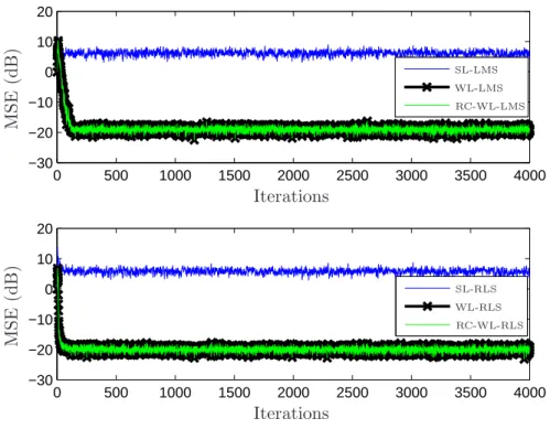
withk = 1,2, ...,5 andβ = 0.432. The desired signal included a Gaussian noise with 20dB signal to noise ratio (SNR). The WL-LMS algorithm used a step-size µWL = 0.04. The RLS forgetting factor was chosen as ν = 0.999 and the initial condition ΦWL(0) = 0.01I. The regressor was generated using both α = 0.1 and α = 1/√2. Note that we define d(n) =Re{wHoptx(n)}, so the widely-linear solution achieves an MSE that is better than that of the SL solution, even when the regressor is proper (since the regressor and desired sequences will not be jointly second-order circular).
0 500 1000 1500 2000 2500 3000 3500 4000 −30 −20 −10 0 10 20
0 500 1000 1500 2000 2500 3000 3500 4000 −30 −20 −10 0 10 20 M S E (d B ) M S E (d B ) Iterations Iterations SL-RLS SL-LMS WL-RLS WL-LMS RC-WL-LMS RC-WL-RLS
Figure 2: MSE for WL and RC-WL algorithms with circular input (α = 1/√2). On the top: SL-LMS, WL-LMS and RC-WL-LMS (µRC = 2µWL = 0.08). On the bottom: SL-RLS, WL-RLS and RC-WL-RLS (ΦRC(0) =ΦWL(0)/2 = 0.005I)
0 500 1000 1500 2000 2500 3000 3500 4000 −30 −20 −10 0 10 20
0 500 1000 1500 2000 2500 3000 3500 4000 −30 −20 −10 0 10 20 M S E (d B ) M S E (d B ) Iterations Iterations SL-RLS SL-LMS WL-RLS WL-LMS RC-WL-LMS RC-WL-RLS
2.4
Conclusions
3
REDUCED-COMPLEXITY QUATERNION
ADAPTIVE FILTERS
Quaternion numbers [3] were invented by Hamilton in the 19th century, as a general-ization of complex numbers to a higher-dimensional domain. They consist of one real part and three imaginary elements, usually identified by i,j and k, where i2 =j2 =k2 =−1 and ijk = −1. Quaternions appear in many fields, and their applications have been spreading recently, since they can be used to concisely describe multi-variable data.
Quaternion algebra is traditionally employed to represent rotations in control applica-tions and in image processing. In the first case, quaternion algebra provides mathematical robustness to represent rotations. Its avoidance of the gimbal lock problem [47] (that ap-pears when using Euler angle representations) is exploited by attitude control systems [48, 49]. On the other hand, in image processing, many techniques employ a quaternion-based model to describe images, allowing a concise representation of the color attributes in a single entity [50, 51], and leading to development of many quaternion-based tools, such as [52–54]. In recent applications, quaternions have been applied to help studying DNA structures [55], and to estimate quantities in neural networks [13], beamforming [56] and adaptive filtering [12, 14, 15, 18, 57, 58], among many others. The last field has experimented a large development lately, and a variety of algorithms has been proposed for multi-variable estimation.
full second-order statistics. In this case, widely-linear algorithms [15] can be applied to improve performance.
In the quaternion case, the definition of WL processes has led to the augmented QLMS [14] (which uses the original SL regressor vector and its conjugate as the WL input data) and to WL-QLMS [58], where the SL data vector and three quaternion involutions are the inputs. Later, WL-iQLMS [62] was also proposed as an improved WL-QLMS algorithm. However, for all these WL methods, the input vector is four times the length of the original SL data vector, and thus the computational cost is significantly higher.
Similar to the complex-valued WL algorithms presented in Chapter 2, quaternion WL techniques have redundance of second-order statistics in the autocorrelation matrix. In this chapter, we propose new WL quaternion algorithms which avoid redundant data and thus reduce the computational complexity. To obtain the new algorithms, we develop an unified description for the diverse quaternion gradients proposed in the literature, and we use it to study the convergence of WL-QLMS-based algorithms. We prove that a class of gradients which includes the i-gradient of [59] leads to the fastest-converging WL-QLMS algorithm, under some conditions on the correlation of the input data.
We also use the general quaternion gradient to develop a further reduced-complexity WL adaptive algorithm for real regressors – the RC-WL-iQLMS algorithm. For this pur-pose, we replace the original WL input vector by a real vector, obtained with a concate-nation of the real and the three imaginary parts of the SL input. We show that using this approach, the redundant statistics are avoided, and many quaternion-quaternion compu-tations are substituted by real-quaternion operations, leading to a low-cost technique. We also prove that the fastest-converging WL-QLMS-based algorithm with real-regressor vec-tor corresponds to the four-channel LMS algorithm (4-Ch-LMS) written in the quaternion domain.
The contributions of this chapter can be summarized as follows:
1. We propose a general approach to describe the different quaternion gradients pro-posed in the literature, and show that different definitions for the quaternion deriva-tive may lead to the same quaternion gradient.
two situations: i) when at most two of the quaternion elements in the input vector are correlated; and ii) when the regressor vector is real.
3. Based on the general gradient, we propose a new technique which applies real re-gressor vector: the RC-WL-iQLMS algorithm, with one fourth the complexity of WL-iQLMS.
4. We show that the fastest-converging WL-QLMS algorithm with real regressor vector is our new algorithm, RC-WL-iQLMS. We also show that RC-WL-iQLMS corre-sponds to the 4-Ch-LMS algorithm written in the quaternion domain.
5. We develop a second-order model valid for any WL-QLMS algorithm with a real-regressor vector. The analysis is suitable for correlated and uncorrelated inputs. Concise equations to compute the EMSE (excess mean-square-error) and the MSD (mean square deviation) [45] are also derived.
The chapter is organized as follows. We present a brief review on quaternion algebra and Kronecker products (which are applied in our analysis) in Section 3.1. In Section 3.2, we present basic concepts of quaternion estimation and Q-properness, while Section 3.3 introduces our general approach to write quaternion gradients. We present the new reduced-complexity algorithm in Section 3.3.2, and develop the analysis of QLMS-based algorithms in Sections 3.4.1 and 3.4.2. Simulations are presented in Section 3.5, and in Section 3.6 we conclude the chapter.
3.1
Preliminaries
In this section, we briefly summarize some properties of quaternion algebra and Kro-necker products. These concepts simplify the analysis and the equations derived in this chapter.
3.1.1
Review on quaternion algebra
A quaternion q is defined as
q=qR+iqI+jqJ+kqK,
complex number is that the multiplication in the quaternion fieldQ is not commutative, since [3]
ij=−ji=k, jk=−kj =i, ki =−ik =j, such that for two quaternionsq1 and q2, in general, q1q26=q2q1.
Similar to complex algebra, the conjugate and the absolute value of a quaternion q are given by
q∗ =qR−iqI−jqJ−kqK
and |q|=√qq∗, respectively. We can also define the following involutions of q1
qi ,−iqi=q
R+iqI−jqJ−kqK qj ,−jqj =q
R−iqI+jqJ−kqK qk ,−kqk=q
R−iqI−jqJ+kqK.
The involutions are used in the definition of WL algorithms (e.g. [18], [58], [15]).
These are the main definitions of quaternion algebra used in this chapter. See reference [3] for more details.
3.1.2
Properties of Kronecker products
The Kronecker product [63] is an efficient manner to compactly represent some large matrices which have a block-structure. Given two matrices A and B, the Kronecker product – which is represented by the operator⊗ – is given by
A⊗B,
a11B . . . a1NB ... . .. ... aM1B . . . aM NB
, (3.1)
For the purpose of the analyses performed in this chapter, the most relevant properties of Kronecker products are
1. A⊗(B+C) =A⊗B+A⊗C. 2. α(A⊗B) = (αA)⊗B=A⊗(αB).
3. (A⊗B) (C⊗D) = AC⊗BD, where the number of rows ofC(B) and the number of columns ofA (D) are equal.
4. (A⊗B)−1 =A−1⊗B−1.
5. (A⊗B)T =AT ⊗BT. 6. Tr(A⊗B) = Tr(A)Tr(B).
7. The eigenvalues of (A⊗B), where A is N ×N and B is M ×M, are given by λAlλBm, for l = 1, 2, . . . , N and m = 1, 2, . . . , M, where λAl and λBm are the
eigenvalues ofA and B, respectively.
These properties appear implicitly or explicitly in the analyses that follow. They make the equations easier to manipulate and simplify the interpretation of the resulting expressions.
3.2
Strictly-linear and widely-linear quaternion
estimation
In the context of complex WL estimation, the concept of second-order circularity or properness is required to define when WL algorithms outperform SL ones (see Section 2.1.2.1). For quaternion quantities, this concept can be extended toQ-properness. In this section, we present Q-properness and compare SL and WL quaternion estimation, based on some results of [58] and [61].
Define the N ×1 quaternion data vector
q(n) = qR(n) +iqI(n) +jqJ(n) +kqK(n), (3.2)
whereqR(n),qI(n),qJ(n) andqK(n) are real vectors. Given a desired quaternion sequence d(n), the problem solved by a strictly linear estimator is the computation of wSL(n) in
ySL(n) =w H
SL(n)q(n) (3.3)
which minimizes the mean-square error E{|eSL(n)|2}, where
eSL(n) =d(n)−ySL(n). (3.4)
From the orthogonality principle [32], it must be true that
E{q(n)e∗SL(n)}=0, (3.5)
and substituting eq. (3.4) in (3.5), we get
Using eq. (3.3) in (3.6),wSL(n) must satisfy
CqwSL(n) =pq, (3.7)
where Cq =E{q(n)qH(n)} is the autocorrelation matrix and pq =E{q(n)d∗(n)} is the cross-correlation vector [1].
For a quaternion WL estimator, the data vector is modified to account for the invo-lutions [12], and it is given by2
qWL(n) = col(q(n), qi(n), qj(n) qk(n) ), (3.8)
which is four times the length of the original vector q(n). For this approach, one must find the vector wWL(n) which minimizes the MSE condition E{|eWL(n)|2}, where
eWL(n) = d(n)−yWL(n), (3.9)
yWL(n) =wHWL(n)qWL(n). (3.10)
Again, the orthogonality condition implies that eWL(n) must be orthogonal to all involu-tions, i.e.,
E{qWL(n)e
∗
WL(n)}=0. (3.11)
Using eqs. (3.9), (3.10) and (3.11), we obtain
CWLwWL(n) =pWL, (3.12)
and
CWL=E{qWL(n)q H
WL(n)}=
Cq Cqqi Cqqj Cqqk
CHqqi Cqi Cqiqj Cqiqk
CHqqj CHqiqj Cqj Cqjqk
CHqqk CHqiqk CHqjqk Cqk
, (3.13)
where
Cα =E{ααH}, forα∈ {q(n),qi(n),qj(n),qk(n)} (3.14) and
Cαβ =E{αβH}, forα,β∈ {q(n),qi(n),qj(n),qk(n)} and α6=β. (3.15)
The matrices Cαβ are the cross-correlation terms between q(n) and their involutions.