Simplifying a hydrological ensemble prediction system with a backward greedy selection of members – Part 2: Generalization in time and space

(1)

www.hydrol-earth-syst-sci.net/15/3327/2011/ doi:10.5194/hess-15-3327-2011

Earth System

Sciences

Simplifying a hydrological ensemble prediction system with a

backward greedy selection of members – Part 2: Generalization in

time and space

D. Brochero1,2, F. Anctil1, and C. Gagn´e2

1_{Chaire de recherche EDS en pr´evisions et actions hydrologiques, Department of Civil Engineering and Water Engineering,}

Universit´e Laval, Qu´ebec, G1V 0A6, Canada

2_{Computer Vision and Systems Laboratory (CVSL), Department of Electrical Engineering and Computer Engineering,}

Universit´e Laval, Qu´ebec, G1V 0A6, Canada

Received: 21 February 2011 – Published in Hydrol. Earth Syst. Sci. Discuss.: 11 March 2011 Revised: 27 September 2011 – Accepted: 10 October 2011 – Published: 4 November 2011

Abstract. An uncertainty cascade model applied to stream

flow forecasting seeks to evaluate the different sources of un-certainty of the complex rainfall-runoff process. The current trend focuses on the combination of Meteorological Ensem-ble Prediction Systems (MEPS) and hydrological model(s). However, the number of members of such a HEPS may rapidly increase to a level that may not be operationally sus-tainable. This paper evaluates the generalization ability of a simplification scheme of a 800-member HEPS formed by the combination of 16 lumped rainfall-runoff models with the 50 perturbed members from the European Centre for Medium-range Weather Forecasts (ECMWF) EPS. Tests are made at two levels. At the local level, the transferability of the 9th day hydrological member selection for the other 8 forecast horizons exhibits an 82 % success rate. The other evalua-tion is made at the regional or cluster level, the transferabil-ity from one catchment to another from within a cluster of watersheds also leads to a good performance (85 % success rate), especially for forecast time horizons above 3 days and when the basins that formed the cluster presented themselves a good performance on an individual basis. Diversity, defined as hydrological model complementarity addressing different aspects of a forecast, was identified as the critical factor for proper selection applications.

Correspondence to:D. Brochero

([email protected])

1 Introduction

The competency of probabilistic forecast to encompass the many sources of uncertainty in Hydrological Ensemble Pre-diction Systems (HEPS) has already been demonstrated (Roulin, 2007; Rousset et al., 2007; Vel´azquez et al., 2011). Yet the simultaneous consideration of the uncertainty asso-ciated with both the meteorological inputs and the structural and parametric configuration of the hydrological models can lead to systems consisting of too many members to be com-putationally and operationally implementable.

Nonetheless, reliability as a crucial feature in ensemble forecasting may be achieved through the uncertainty cascade model as proposed by Pappenberger et al. (2005). This ap-proach states that the output uncertainty of a hydrological model is affected by several components: uncertainty from the meteorological data used to drive the model, initializa-tion uncertainty (i.e. the initial state of the model), and the model uncertainty (from parameter identification to model conceptualization).

(2)

turn out to be quite large. Simplification of such a HEPS thus becomes a mandatory step from an operational standpoint.

In such a context, the hydrological and meteorological community has focused their efforts on many lines of simpli-fication. For instance, Pappenberger et al. (2005) evaluated 10-day ahead rainfall forecasts, consisting of one determin-istic, one control, and 50 ensemble forecasts, into a rainfall-runoff model (LisFlood) for which parameter uncertainty was represented by six different parameter sets identified through a Generalized Likelihood Uncertainty Estimation (GLUE) analysis and functional hydrograph classification. Raftery et al. (2005) proposed the Bayesian Model Aver-age methodology (BMA) as a means for the statistical post-processing of the forecast ensembles derived from numeri-cal weather prediction models. The BMA predictive prob-ability density function (PDF) is a weighted average of the PDFs centred on the bias-corrected forecasts from a set of different models. The weights assigned to each model re-flect that model’s contribution to the forecasting skill over a training period (Vrugt et al., 2006). In line with that, Vrugt et al. (2008) proposed evaluating BMA weights with the Dif-feRential Evolution Adaptive Metropolis (DREAM) Markov Chain Monte Carlo (MCMC) algorithm.

Other studies identified the meteorological forecasts as the most uncertain component of the cascade model (Todini, 2004; Pappenberger et al., 2005; Jaun et al., 2008), trigger-ing interest in novel member selection techniques. For ex-ample, Marsigli et al. (2001); Molteni et al. (2001) and Jaun et al. (2008) select MEPS members based on lagging en-sembles, and derived representative members through hier-archical clustering over the domain of interest. Ebert et al. (2007) analysed the relation between the atmospheric circu-lation patterns and extreme discharges to select representa-tive members of MEPS. Finally, Xuan et al. (2009) establish, in a deterministic way (“best match” approach), the location of the forecast that is the most similar to the rainfall pattern of the catchment.

In the companion paper, Brochero et al. (2011) described in depth the hydrological member selection methodology adopted here: a Backward Greedy Selection combined with Cross Validation, hereafter BGS-CV, to retain the uncer-tainty properties of a 800-member HEPS derived from the fifty members of the European Center for Medium-range Weather Forecasts (ECWMF) propagated through sixteen simple lumped hydrological models.

Another aspect of particular interest in the evaluation of probabilistic forecast, and therefore in hydrological member selection, is the identification of a pertinent criteria set. In conventional forecasting, i.e. when confronting an observa-tion against a single predicobserva-tion, it is now generally accepted that the calibration of hydrological models should be ap-proached as a multi-objective problem (Gupta et al., 1998, 1999; Yapo et al., 1998; Wagener et al., 2001; Confesor and Whittaker, 2007). Probabilistic forecasting is not different in that regard. In fact, the complexities of confronting an

observation against an ensemble of predictions calls for a va-riety of criteria, here called scores, that specifically focus on one or more characteristics of the probabilistic sets. So, to assess these properties, several statistical measures should be considered concurrently (Wilks, 2005; Cloke and Pappen-berger, 2009). Few studies have experimented hydrological member selection from a multi-score point of view.

Vrugt et al. (2006) posed the BMA inverse problem in a multi-objective framework, examining the Pareto set of so-lutions between the Continuous Ranked Probability Score (CRPS), the Mean Absolute Error (MAE), and the Ignorance Score with the AMALGAM method (Vrugt and Robinson, 2007). In continuity with that, the companion paper shows that a combined criterion which groups various characteris-tics of the probabilistic forecast is adequate to guide the se-lection of hydrological members with BGS-CV method. At this point, it is important to note that the BGS-CV method of-fers the possibility of combining results from different stud-ies, which is highlighted as one of the aspects related to the improvement of HEPS (Cloke and Pappenberger, 2009).

In this paper we evaluate the generalization of a simplifi-cation scheme of the complex 800-member HEPS presented in Sect. 2. A brief description of the selection of hydrologi-cal members is given in Sect. 3. The generalization method-ology, with local and regional orientation, is explained in Sect. 4. Thus, we test the hydrological members’ selection obtained in sixteen catchments for the 9-day lead time, for the other 8 lead times. Additionally we evaluate the abil-ity to extrapolate the selections to neighbouring catchments. Finally we present the integration of results from different catchments within a regional framework. Results and discus-sion are gathered in Sect. 5, while concludiscus-sions and a guide-line for future work are given in Sect. 6.

2 HEPS configuration and catchment locations

As already mentioned, the 800-member HEPS at hand is the propagation of 50 perturbed members from the ECMWF EPS, that are a priori assumed to be equally likely (Gouweleeuw et al., 2005), through sixteen lumped hydro-logical models. Details of the HEPS conformation can be found in Brochero et al. (2011).

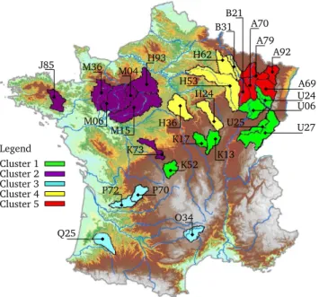
This HEPS was implemented over 28 French catch-ments, representing a large range of hydro-climatic condi-tions (Fig. 1), and evaluated over a 17-month period. The main characteristics of these catchments are summarized in Table 1. Henceforth each basin in Table 1 will be identified only with the first three characters.

(3)

Table 1.Main characteristics of the studied basins (mean annual values) based on a 36 year length of the series (1970–2006).

Catchment Area P ET Q Catchment Area P ET Q

codes (km2) (mm) (mm) (mm) codes (km2) (mm) (mm) (mm)

A6921010 2780 3.04 1.79 1.18 M0680610 7380 2.04 1.93 0.56

A7930610 9387 2.78 1.80 1.21 O3401010 2170 3.19 1.80 1.90

A9221010 1760 2.49 1.83 0.91 Q2593310 2500 2.52 2.24 0.75

B2130010 2290 2.57 1.80 0.87 U2542010 4970 3.63 1.75 1.88

B3150020 3904 2.58 1.80 1.09 A7010610 6830 2.99 1.78 1.46

H2482010 2982 2.31 1.89 0.84 H6221010 2940 2.50 1.83 0.92

H3621010 3900 1.98 1.95 0.45 M3600910 3910 2.31 1.88 0.80

H5321010 8818 2.41 1.85 0.93 K1341810 2277 2.65 1.89 1.02

J8502310 2465 2.36 1.89 0.81 M1531610 7920 1.85 1.95 0.36

K1773010 1465 2.65 1.94 1.07 P7001510 1863 2.88 2.08 1.19

K7312610 1712 2.13 2.01 0.68 P7261510 3752 2.65 2.14 0.87

M0421510 1890 2.04 1.89 0.62 U2722010 7290 3.63 1.79 2.07

P: precipitation, ET: potential evapotranspiration, Q: flow. For the distinction of the basins used in training and testing, the latter are highlighted in bold.

A79 B21 B31

U25 H36

O34 Q25

K73 M04 J85

A92 A70

H62

H53 A69

U24

U27 U06 H24

K13 K17

P70 P72

H93

M15 M06 M36

K52 Legend

Cluster 1 Cluster 2 Cluster 3 Cluster 4 Cluster 5

Fig. 1. Location of the catchments grouped by clusters. Some of them have been used in the BGS-CV process, while the others have been used for extrapolation. The colours identify the five regions evaluated in this paper.

conceptualizations of the sixteen hydrological models used. It should be clear that the comparison would not be fair be-cause some models such as the GR4J were specifically de-vised for the catchment scale, whereas others have suffered a series of substantial changes bringing them to a lumped state.

3 Hydrological members’ selection

The hydrological members’ selection is described in detail in the companion paper (Brochero et al., 2011). It is executed basically in three steps:

Step 1: Resampling with a variation of the k-fold

cross-validation. Because the series are short-length (500

forecast-observation pairs), a rigorous application of the selection re-quires evaluating different types of events in the training, val-idation, and test sets. Thus, the process of selecting data fol-lows ak-fold cross-validation technique.

Step 2: Backward greedy selection. Optimization for

a preselected number of hydrological members (nmim) re-lies on the Combined Criterion (CC), which brings together the Continuous Ranked Probability Score (CRPS), the IGNo-rance Score (IGNS), the Mean Squared Error (MSE) evalu-ated in the Reliability Diagram (RD), theδratio evaluated in the rank histogram and the MeDian of Coefficients of Varia-tion (MDCV):

CC = w1

CRPSse

CRPSie

+w2

z1−IGNSse

z1 −IGNSie

(1)

+w3

RDMSEse

RDMSEie

+w4

δse

δie

+w5

z2 −MDCVse

z2 −MDCVie

,

where the result of each criterion in the selection ensem-ble (se subscript) is divided by the criterion calculated on the initial 800-member HEPS (ie subscript). zm represents

some thresholds to orient a direct minimization;wcpare the

weights assigned to each component. Here, the weight as-signed to the reliability (the critical factor) is twice that of the other factors, which have a unit weight.

(4)

that, when it is removed, has the greater impact on the train-ing set error (i.e. minimises traintrain-ing error the most).

Step 3: Combination of results. It is highly likely that

vari-ability in the five experiments configured in the first step will lead to different solutions. An integration mechanism is thus needed for a global solution for each catchment. The im-portance of each hydrological member within the ensemble is then assumed as being directly proportional to the itera-tion number at which it was eliminated during the selecitera-tion process in each experiment.

Attention is given to the interpretation of results of the final hydrological members’ selection, because if the HEPS is driven by a MEPS with interchangeable members (e.g. ECMWF EPS), the selection should be directed more clearly to a method of selection and weighting of hydrolog-ical models based on their participation in the final selected subset. Therefore, in the simplest case, we can create a new simplified high-performance HEPS using the same propor-tion of the hydrological members associated with a random choice of the meteorological members.

Note that the CC could be used to compare the perfor-mance of the hydrological members’ selection with respect to the 800-member set. So, in a general framework, if all features of the ensemble forecast have the same importance, one members’ selection with equal performance to the 800-member set will lead to a CC equal to 5, values lower than 5 indicate a selection of higher performance than the base set of 800 members, and values greater than 5 indicate the detri-ment of some feature of the 800-member set. Hereafter, this particular condition of unit weights in the CC will be called the normalized sum (NS). This distinction is important to dis-play the priority that can be defined a priori to any feature in the hydrological members’ selection training with BGS-CV. It is important to note that the normalized sum may hide some deterioration compensated by one or more other met-rics. It is thus necessary to accompany this measure with the results of each of its components, for a collective analysis. In this sense, the analysis is facilitated if each component is associated with an index that reflects the gain or loss of the selected subset over the initial 800-member set:

Gain(%) =100 × Scoreie −Scorese |Scoreie|

. (2)

Note that the absolute value is used in the denominator for accounting for possible negative values of the IGNS. The MDCV function further requires the inversion of the numer-ator, because the purpose of this metric is to maximize the dispersion of the selected subset of hydrological members.

4 Generalization test methodology

The generalization ability of a hypothesis, namely, the qual-ity of its inductive bias, can be measured if there is access to data outside of the training process. The methodology pro-posed in the companion paper simulates this by dividing the

training set into two parts. One part is used for training (i.e. to find a hypothesis) and the remaining part (validation set) is used to test the generalization ability. Nevertheless, if it is necessary to report the error to approximate the expected se-lection error, it is compulsory to make use of a third set, a test set, sometimes also called the publication set, containing ex-amples not used in training or validation (Alpaydin, 2010; Hudson and Demuth, 2011).

Thus, the method of combining results, based on the mean rank of elimination, is derived on the use of all series as a means of optimizing the use of information in a short-length series (seen from the point of view of the periodicity of the hydrological cycle). However, results of this procedure can be conceived as indicators of a relative performance or otherwise as an optimistic estimate of the hydrological mem-bers’ selection process (Diamantidis et al., 2000).

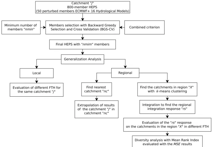
Figure 2 shows the generalization or test methodology of the hydrological members’ selection at two levels: the lo-cal focuses on the extrapolation of results to different FTH within the same catchment and another named regional, while the regional level tests the temporal and spatial perfor-mance in nearby catchments, or under a broader perspective on the integration of regional results.

4.1 Extrapolation to different forecast time horizons

The hydrological members’ selection is performed on the results of sixteen hydrological models fed with the 9th day FTH of the ECMWF MEPS. Thus, the application of this se-lection of members for the other eight FTHs (1 to 8 days) is a first level test. It has to be stressed that the idea of simpli-fying the HEPS is only valuable if the hydrological member selection is invariant in regard to the FTH. However, one may always argue that the assumption of statistical independence between the test and training data, principally for FTHs next to the ninth, may be somewhat questionable.

4.2 Extrapolation to a different catchment

Transferring selected members to a neighbouring catchment, and even further to a different FTHs, constitutes a rigorous test of the generalization ability of results at both the tempo-ral and spatial scales. The choice of the second catchment could first be viewed as a simple nearest neighbour prob-lem. However, we explored the possibility of regionalizing the selection of hydrological members from the grouping of catchments by k-means clustering and subsequent integra-tion of results to select the most representative hydrological members.

4.2.1 k-means clustering

(5)

Fig. 2.Generalization test methodology for the hydrological members’ selection found with BGS-CV.

evapotranspiration and flow (see Table 1). Of course, every possible combination of features will yield a different distri-bution of catchments that will be evaluated through the inte-gration mechanism that will be presented in Sect. 4.2.2.

It is convenient at this point to define some notation to describe the assignment of catchments to a region or clus-ter. The property setxl_{for each catchment is introduced into}

a corresponding set of binary indicator variablesbl_k∈ {0,1}, wherek= 1, ...,Kdescribe which of theKclusters the catch-mentl or its property setxl _{is assigned to, so that if}_xn _is assigned to clusterkthenb_kn= 1, andbn_j= 0 forj6=k. Then an objective function is given by:

J =

L

X

l=1

K

X

k=1

b_klkxl −m_kk2, (3)

which represents the sum of the squares of the distances of each catchment to its assigned vectorm_{k. The goal is to find}

values for thebl_k and them_k _{so as to minimise}J. Then the iterative application of Eq. (3) leads to the following proce-dure for finding them_k_centres:

Algorithm 1k-means pseudo-code

1. Define the number of clusters (K), (hereK= 5) 2. Initialize randomly centresm_k ₍_k_{= 1,}_···_,_K₎

repeat

forallxl_, _l_{= 1,}_..._,_L_do

b_kl = (

1 l = argmin_kkxl ₋m_k_k

0 otherwise

end for

forallm_k_do

m_k =

PL l=1blkxl

bl_k

end for

untilm_k_converges

Details of thek-means clustering algorithm are given by Bishop (2006). Figure 1 shows an example ofk-means clus-tering results based only on the geographic location of the basin outlets.

4.2.2 Regional integration mechanism

(6)

S, which hasC columns withnmin rows representing the mostnmin important hydrological members as assessed by the mean rank of elimination (R) for each catchment. Then, the process of forming a regional solutionrs withq mem-bers is based on taking the most important memmem-bers of each catchment without replacement until the number of members inrsis equal to the desiredq, i.e. each member cannot be se-lected again later. Algorithm 2 details this procedure:

Algorithm 2Regional integration mechanism pseudo-code

1. Determine theCcatchments in theXregion (clustering process).

2. Define the matrixS={s1,s2, ···,sC}

3. Establish the number of hydrological membersqin the regional solutionrs

4. Initializers={}, h= 0 andi= 1

repeat

forj= 1, ..., Cdo

ifSi,j ∈/ rs then

rs=rs+Si,j

h=h+ 1

end if end for

i=i+ 1

untilh > q

4.2.3 Diversity evaluation

The participation of hydrological models in the regional se-lection stresses the importance of the integration of models with different characteristics. To view this in a deterministic framework, an index based on the performance rank assigned to each model in each catchment is proposed. Its calculation is summarized as follows:

– MSE for catchmentiand hydrological modelj is first calculated (MSEi,j).

– Performances are next ranked for each catchment, lead-ing to PRi,j, for which the model with the lowest MSE is assigned the rank PR = 16 and the highest MSE is as-signed the rank PR = 1.

– Finally, the mean rank of performance or rank index RIj for each model is estimated based on the results of all 28 basins:

RIj = 1

28

28 X

i=1

PRi,j. (4)

5 Results and discussion

In the companion paper we have shown the high performance of the 800-member HEPS for the 9th day FTH. However, as

one of the objectives of this paper is to show the transferabil-ity of the hydrological members selections to other FTHs, it is necessary to show the performance of the 800-member HEPS in such scenarios to clearly establish our point of ref-erence concerning the quality of the hydrological members’ selection. In the companion paper we also stressed that on theδratio and the RDMSEscores rest the main advantages of

the 800-member HEPS.

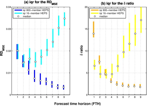
Figure 3 shows the HEPS’ behaviour with different set-up and different FTH. Results focus on the reliability (RDMSE)

and the ensemble consistency (δ ratio) for two schemes formed from sixteen hydrological models, one led by the de-terministic ECMWF forecast and the other by the 50 per-turbed members from ECMWF EPS. The results in Fig. 3, expressed in terms of interquartile range (iqr) and median, are due to the grouping of the scores obtained in the 28 basins evaluated here. Note that theδratio and RDMSE scores are

directly comparable since their scale is independent of the measured variable.

Figure 3 illustrates that the 800-member HEPS advan-tages becomes apparent after the 4th day FTH. According to Vel´azquez et al. (2011), part of this difficulty may be inher-ited from the meteorological ensembles, which are not reli-able prior to about a 3-day lead time. Furthermore the spread in the results of both the RDMSE and the δ ratio, viewed

from the interquartile range, shows two features: first, the 16-member HEPS has greater dispersion than the 800-16-member HEPS, and second, the 800-member HEPS spread dimin-ishes with increasing lead time.

5.1 Selection process

The optimal number of hydrological members simplifying the HEPS was identified in the companion paper to be be-tween 50 and 100, depending on the catchment. In most cases a significant gain with respect to the balance of the dif-ferent criteria evaluated from the initial 800-member HEPS was then achieved. Results presented in this section are based on a selection of 50 hydrological members.

Table 2 presents the results of the 50-member selection based on the combined criterion, for 16 catchments uni-formly distributed over France (see Fig. 1). The overall per-formance is the normalized sum given by Eq. (1) with unit weights definition, values lower than 5 indicate a selection of higher performance than the base set of 800 hydrological members, and values greater than 5 indicate the detriment of any feature of the 800-member set.

(7)

1 2 3 4 5 6 7 8 9 0

0.01 0.02 0.03 0.04

(a) iqr for the RD_MSE

RD

MSE

iqr 800−member HEPS iqr 16−member HEPS median

1 2 3 4 5 6 7 8 9

0 0.01 0.02 0.03 0.04

(a) iqr for the RD_MSE

RD

MSE

1 2 3 4 5 6 7 8 9

0 5 10 15 20

(b) iqr for the δ_ratio

δ

ratio

Forecast time horizon (FTH)

iqr 800−member HEPS iqr 16−member HEPS median

1 2 3 4 5 6 7 8 9

0 5 10 15 20

(b) iqr for the δ_ratio

δ

ratio

Fig. 3.Interquartile range (iqr) of RDMSEandδratio assessed in the 28 catchments under two HEPS schemes: 16-member HEPS (16 hy-drological models are driven by the deterministic forecast from ECMWF) and the 800-member HEPS (16 hyhy-drological models are driven by the 50-perturbed member forecast from ECMWF).

Table 2 shows that in all cases the normalized sum (NS) is always lower than 5, indicating the superiority of the 50-member HEPS, even after a size reduction equivalent to a 94% compression of the initial 800-member HEPS (i.e. 750 members are removed).

Based on the gain score formulation (Eq. 2), it is noted that for the 50-member selection, the CRPS and the MDCV show low variability with mean gain indexes around 2 % and 5 %, respectively.

RDMSE shows a minimum gain of 49 % (catchment B21)

and a maximum gain of 87 % (catchment K17), reflecting the emphasis given to this property in the formulation of the combined criterion used in the selection process. With re-spect to the IGNS, index gains between−5 % and 27 % (ex-cluding the catchment B21) reflect an acceptable behaviour.

Finally, theδratio is the score more difficult to minimise or preserve; a positive index gain was obtained for only 25% of the cases (4/16), while the spread ranged from−39 % for catchment H53 to 27 % for catchment B31. Note that theδ ratio has an inverse relationship with the number of mem-bers of the selection, so it directly follows the complexity in maintaining the value of the initial 800-member HEPS in the selection process. Nonetheless, it was shown in the compan-ion paper that theδratio is the best individual metric for the hydrological members’ selection.

5.2 Generalization test

5.2.1 Local analysis

For operational convenience, it is fundamental that the 50 hy-drological members selected for the 9th day FTH are also ap-propriate for the 8 previous time horizons. A lack of transfer-ability of the selected members would considerably reduce the actual level of achieved simplification.

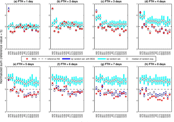
Here, temporal transferability is first evaluated comparing the normalized sum of the performance of the 50-member se-lection to the 800-member performance, whose normalized sum equals 5 in all cases. It is then compared to the per-formance of 200 random combinations with 50 hydrological members, in order to evaluate if any good performance may only be attributable to chance. Results for the 8 first FTHs and sixteen basins are gathered in box-plot diagrams (Fig. 4), where the performance of the solution is based on random experiments that are set-up following these guidelines:

– Experiments considering the participation of hydrologi-cal models found with BGS-CV: taking into account the participation of hydrological models to assign to each model a number of members chosen randomly from ECMWF EPS.

(8)

Table 2.Selection of 50 hydrological members based on combined criterion and the BGS-CV process on the 9-day FTH. Beside each score is presented the gain index evaluated by Eq. (2). NS represents the normalized sum (Eq. 1 with unit weights). NHM indicates the number of hydrological models participating in the selection. RDMSEvalues are expressed on a 10−3basis.

Catchment Codes

Scores MDCV

function NS NHM

CRPS RDMSE δ IGNS

A69 0.284 (+0 %) 1.3 (+81 %) 1.5 (+18 %) 0.67 (+14 %) 0.39 (+5 %) 4.0 9

800 members 0.284 7.0 1.8 0.78 0.37 5.0 16

A79 0.254 (+3 %) 1.5 (+69 %) 3.6 (−11 %) 0.34 (+23 %) 0.41 (−1 %) 4.4 11

800 members 0.263 5.1 3.3 0.44 0.41 5.0 16

A92 0.183 (+4 %) 0.3 (+86 %) 2.3 (−28 %) −0.42 (+27 %) 0.57 (+0 %) 4.4 11

800 members 0.192 2.4 1.8 −0.33 0.57 5.0 16

B21 0.232 (−1 %) 1.2 (+49 %) 2.6 (−16%) −0.18 (−38%) 0.63 (+9 %) 4.6 13

800 members 0.230 2.4 2.2 −0.29 0.57 5.0 16

B31 0.134 (+1 %) 1.3 (+72 %) 2.0 (+27 %) −0.84 (−5 %) 0.24 (+7 %) 4.0 11

800 members 0.135 4.5 2.7 −0.88 0.22 5.0 16

H36 0.157 (+2 %) 0.7 (+80 %) 2.0 (−37%) −1.02 (+2 %) 0.36 (−1 %) 4.5 14

800 members 0.161 3.5 1.5 −0.99 0.37 5.0 16

H53 0.165 (+3 %) 1.9 (+74 %) 4.3 (−39 %) −0.76 (+8 %) 0.36 (+8 %) 4.6 11

800 members 0.171 7.4 3.1 −0.71 0.33 5.0 16

H24 0.180 (+2 %) 2.2 (+68 %) 3.8 (−32%) −0.82 (+9 %) 0.37 (+6 %) 4.6 12

800 members 0.185 7.1 2.9 −0.76 0.35 5.0 16

K17 0.205 (+4 %) 0.5 (+87 %) 1.8 (−9 %) −0.73 (+12 %) 0.38 (−2 %) 4.2 12

800 members 0.213 3.6 1.7 −0.65 0.39 5.0 16

U25 0.290 (+0 %) 0.9 (+74 %) 2.6 (−1 %) −0.40 (+13 %) 0.38 (+7 %) 4.2 14

800 members 0.289 3.4 2.5 −0.36 0.35 5.0 16

J85 0.159 (+2 %) 0.4 (+80 %) 1.7 (−5 %) −1.00 (+2 %) 0.40 (+8 %) 4.2 14

800 members 0.163 2.2 1.7 −0.98 0.37 5.0 16

K73 0.160 (+3 %) 0.9 (+70 %) 2.1 (−5 %) −0.93 (+0 %) 0.38 (+9 %) 4.3 11

800 members 0.165 3.1 2.0 −0.93 0.35 5.0 16

M04 0.158 (+1 %) 0.6 (+68 %) 1.6 (−2 %) −0.98 (−1 %) 0.37 (+2 %) 4.3 13

800 members 0.160 1.7 1.6 −0.99 0.37 5.0 16

M06 0.153 (+4 %) 0.3 (+79 %) 1.6 (−4 %) −1.09 (+6 %) 0.39 (+1 %) 4.2 13

800 members 0.159 1.4 1.5 −1.03 0.38 5.0 16

O34 0.166 (+2 %) 1.0 (+71 %) 1.6 (+1 %) −0.91 (+5 %) 0.37 (+3 %) 4.2 13

800 members 0.169 3.5 1.6 −0.86 0.36 5.0 16

Q25 0.159 (+3 %) 0.6 (+73 %) 1.1 (+22 %) −0.94 (−5 %) 0.39 (+4 %) 4.0 12

800 members 0.163 2.1 1.4 −0.98 0.37 5.0 16

Figure 4 shows that the median of 200 evaluations of 50-member HEPS for the 9th day FTH is superior to the 800 ref-erence members in 82 % of the evaluated cases. It is also noteworthy that in only 11 % of the cases (14/128) the 50 hy-drological members selected oriented by the BGS-CV pro-cess lead to a worse performance than the 25 percentile of 200 random combinations test. Note that all these cases cor-respond to short lead times (1 to 3 days), remarkably in the 2-day FTH. Another aspect that draws attention is the low dispersion of the BGS-CV selections represented by the in-terquartile range, highlighting the importance of the hydro-logical models participation in the selection process.

Figure 4 also shows that the selection slowly loses effi-ciency as it moves away from the 9th day FTH. It also detects a systematic deficiency for catchment A69 and to a lesser ex-tent for catchment B21. Nonetheless, these results are very encouraging.

5.2.2 Regional analysis

(9)

3 4 5 6 7

(a) FTH = 1 day

A69 A79 A92 B21 B31 H24 H36 H53 J85 K17 K73 M04 M06 O34 Q25 U25

3 4 5 6 7

(b) FTH = 2 days

3 4 5 6 7

(c) FTH = 3 days

3 4 5 6 7

(d) FTH = 4 days

3 4 5 6 7

(e) FTH = 5 days

3 4 5 6 7

(f) FTH = 6 days

3 4 5 6 7

(g) FTH = 7 days

3 4 5 6 7

(h) FTH = 8 days

Catchments

Normalized sum (reference value = 5)

BGS reference NS iqr random sel. with BGS iqr random sel. median of random exp.

Fig. 4.Evolution of the normalized sum (NS) to evaluate the response sensibility with regard to the interquartile range (iqr) of 200 random experiments in different FTHs following these guidelines: (1) Considering the participation of hydrological models found with BGS-CV (vertical blue bars), and (2) Without regard to any “a priori” participation of hydrological models, i.e. completely random selection (vertical cyan bars).

selection obtained for catchment Q25 for a lead time of 9 days to catchment P72 for the 4-day lead time.

In general, Fig. 5 shows that results for the different scores are very similar for the 800-member and 50-member sets, ex-cept for the RDMSE where the gain index reaches 51 %. In

particular, Fig. 5a shows that the 50-member CRPS equals the reference value. Taking into account that the CRPS gen-eralizes the mean absolute error (CRPS) for a point forecast (Gneiting and Raftery, 2007), it is important to stress that the CRPS values are always lower than the MAE values, when the deterministic counterpart was taken as the mean of each daily ensemble, in agreement with results obtained by other authors (Boucher et al., 2009; Vel´azquez et al., 2011).

Another remarkable feature of CRPS is its direct relation-ship with the flow magnitude; the shapes of the CRPS and of the hydrograph are similar.

A direct strategy of optimization could then focus on removing the hydrological members that have a large im-pact on the daily extreme CRPS values. Note also that the

selection not only preserves the mean CRPS (0.16) but also the structure of the CRPS series.

Figure 5b shows that the trimmed mean IGNS for the 50-member HEPS (−1.65) also presents an improvement over the initial value (−1.59). Regarding the time structure of the IGNS, it is observed that both the 50-member and 800-member series have high values for extreme events, showing a systemic problem in terms of ensemble bias.

(10)

11/03 19/06 27/09 05/01 15/04 24/07 0.0 0.8 1.6 2.5 3.3 4.1 Time [days]

(a) CRPS = 0.13 mm , MAE = 0.16 mm

mean CRPS [mm]

11/03 19/06 27/09 05/01 15/04 24/07 0.0 0.8 1.6 2.5 3.3 4.1 Time [days]

(a) CRPS = 0.13 mm , MAE = 0.16 mm

0.0

8.3 Observed flow

800−member

50−member

11/03 19/06 27/09 05/01 15/04 24/07

−6.6 35.5 77.7 119.8 161.9 204.0 Time [days]

(b) IGNS = −1.65 bits

mean IGNS [bits]

11/03 19/06 27/09 05/01 15/04 24/07 −6.6 35.5 77.7 119.8 161.9 204.0 Time [days]

(b) IGNS = −1.65 bits

0.0

8.3

Observed flow [mm]

Observed flow

800−member

50−member

0 0.2 0.4 0.6 0.8 1

Forecast probability, (I

m)

Conditional event relative frequency, p(o

t|Im

)

(c) Reability Diagram error, RD(e−3) = 4.21

800−member 50−member

0 0.2 0.4 0.6 0.8 1

Forecast probability, (I

m)

Conditional event relative frequency, p(o

t|Im

)

(c) Reability Diagram error, RD(e−3) = 4.21

1 10 20 30 40 51

0 7 14 21 28 35 Rank Occurrences

(d) δ = 3.1, MDCV = 0.16

50−member href

1 10 20 30 40 51

0 7 14 21 28 35 Rank Occurrences

(d) δ = 3.1, MDCV = 0.16

0 5 10

HM01 HM02 HM03 HM04 HM05 HM06 HM07 HM08 HM09 HM10 HM11 HM12 HM13 HM14 HM15 HM16 Occurrences ID Model

(e) Models’ participation

0 5 10

HM01 HM02 HM03 HM04 HM05 HM06 HM07 HM08 HM09 HM10 HM11 HM12 HM13 HM14 HM15 HM16 Occurrences ID Model

(e) Models’ participation

Opt. criterion = CC. Train = Catchment Q2593310 − FTH = 9. Test = Catchment P7261510 − FTH = 4 Reference values (800 members) P7261510 → CRPS = 0.132, RD(e−3) = 8.67, δ = 3.2, MDCV = 0.15, IGNS = −1.59

Fig. 5.Comparison between the initial ensemble (800 members) and the ensemble selected (50 members) for a lead time of 9 days.(a)Figure above: observed flow; figure below: CRPS (x-axis formatted as: day/month). Note the correspondence between higher observed flows and higher CRPS.(b)Figure above: observed flow; figure below: IGNS (x-axis formatted as: day/month). (c)Reliability diagram error (MSE based on vertical distances between the points). (d)Rank histogram for the 50 hydrological members selected. The horizontal dashed line indicates the frequency (N/d+ 1) attained by a uniform distribution. (e)Occurrences of the employed models in the final solution of 50 hydrological members.

Figure 5e illustrates the occurrence of each lumped model within the 50-member hydrological ensemble. A wide selec-tion of models alone could justify the multi-model approach advocated here. Results show that 12 models out of 16 were selected in this case, and that no models were selected more than 9 times. Knowing that these models are not of equal quality with regards to MSE performance, for instance, this suggests that the selection favoured a diversity of errors. At the end of the selection process, the MDCV has slightly in-creased, from 0.15 to 0.16.

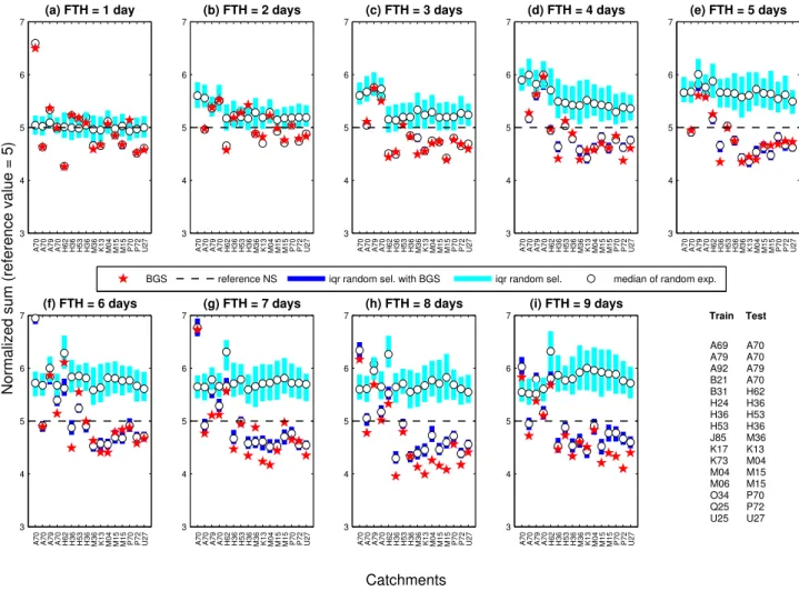
To display an overview of the extrapolation of results to the nearest basin, Fig. 6 shows such an assessment under the same selection schemes analysed in Fig. 4, i.e. analyzing

various combinations considering or ignoring the solution found with BGS-CV. Although in general the solution found with BGS-CV (red stars in Fig. 5) exhibits the highest per-formance, given the interchangeability of MEPS members as input of hydrological models, solutions focus on comparing the median of the evaluations that follow the participation of hydrological models found with BGS-CV.

(11)

3 4 5 6 7

(a) FTH = 1 day

A70 A70 A79 A70 H62 H36 H53 H36 M36 K13 M04 M15 M15 P70 P72 U27

3 4 5 6 7

(b) FTH = 2 days

3 4 5 6 7

(c) FTH = 3 days

3 4 5 6 7

(d) FTH = 4 days

3 4 5 6 7

(e) FTH = 5 days

3 4 5 6 7

(f) FTH = 6 days

3 4 5 6 7

(g) FTH = 7 days

3 4 5 6 7

(h) FTH = 8 days

3 4 5 6 7

(i) FTH = 9 days

Catchments

Normalized sum (reference value = 5)

Train

Test

BGS reference NS iqr random sel. with BGS iqr random sel. median of random exp.

Fig. 6.Evolution of the normalized sum (NS) to evaluate the response sensibility of the extrapolation of results in the nearest catchments. Each vertical bar represents the interquartile range (iqr) of 200 combinations of 50 hydrological members under the following guidelines: the combination is oriented with the same proportion of hydrological models found with BGS-CV (blue vertical bars), the selection is completely random (cyan vertical bars). Note the deficiency of the selections’ extrapolation in basin A69 to basin A79, notably for early lead times (2 to 5 days); these results do not appear in the figure because they are above 7.

Another aspect that stands out in the extrapolation is the recurrent deficiency of selection in the basins A69, A92, B21 and B31, i.e. 25 % of the basins tested. Initially, the deficiency in these basins at different FTHs shows the tem-poral consistency of HEPS, as if the deficiency of a given selection disappears at certain lead times would reflect in-consistency of the selection task.

Likewise, it is noteworthy that extrapolation of the results of selection in the basins A69, A79 and B21 are tested in the basin A70; however, only the results of the hydrological members’ selection in the basin A79 show considerable effi-ciency in most of the FTHs evaluated. It follows that while the geographic location of the basin outlet is an acceptable feature to run the extrapolation of results, it is not sufficient in some cases, which requires a more detailed analysis of other factors such as hydrometeorological and physiographic characterization of the basins.

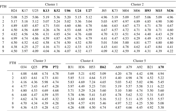
The regional analysis that integrates several basins, which seeks to identify features that facilitate the combination of results, revealed that geographical location is the most im-portant feature, followed by evapotranspiration, precipitation and flow, when the normalized sum is used to evaluate the gain. However, consideration of the geographic location was found to be sufficient. Such results are presented in Table 3, after application of thek-means algorithm and the regional integration procedure already described in Sect. 4.2.2.

Note that the results in Table 3 are due to the evaluation of one combination of MEPS members randomly chosen, but respecting the participation of hydrological models found with BGS-CV. Additionally, for purposes of extrapolation of results, in the evaluation of the normalized sum, a threshold z1equal to−4 was used, because in the first lead times (1 to

(12)

Table 3.Test based on the normalized sum in new catchments and different FTHs of regional integration given by the analysis of clusters by geographical location of the basin outlets. Values lower than 5 determined that the scores of selection are better than the reference set. See clusters’ distribution in Fig. 1. In each cluster, the catchments highlighted in bold represent the series that are not used by the hydrological members’ selection training methodology.

FTH Cluster 1 Cluster 2

H24 K17 U25 K13 K52 U06 U24 U27 J85 K73 M04 M06 H93 M15 M36

1 5.08 5.25 5.06 5.19 5.36 5.20 5.15 5.12 4.96 5.19 5.09 5.07 5.06 5.09 4.96

2 5.17 5.18 5.12 5.07 5.24 5.02 5.36 5.04 5.03 4.97 4.97 4.89 4.85 4.90 5.00

3 4.89 4.85 4.87 4.71 5.01 4.60 4.86 4.78 4.66 4.63 4.67 4.73 4.71 4.70 4.67

4 4.50 4.56 4.69 4.26 4.76 4.53 4.68 4.59 4.67 4.57 4.72 4.71 4.70 4.71 4.60

5 4.82 4.56 4.56 4.31 4.85 4.54 4.76 4.68 4.70 4.33 4.51 4.54 4.40 4.43 4.29

6 4.99 4.74 4.86 4.59 4.87 4.59 4.76 4.79 4.41 4.47 4.53 4.29 4.49 4.53 4.34

7 4.50 4.52 4.42 4.58 4.74 4.50 4.52 4.50 5.01 5.04 5.00 4.81 4.77 4.80 4.80

8 4.38 4.25 4.27 4.16 4.71 4.22 4.33 4.33 4.43 4.61 4.78 4.62 4.47 4.84 4.41

9 4.50 3.97 4.09 4.04 4.36 4.07 4.32 4.17 4.09 4.32 4.59 4.39 4.31 4.39 4.22

FTH Cluster 3 Cluster 4 Cluster 5

O34 Q25 P70 P72 B31 H36 H53 H62 A69 A79 A92 B21 A70

1 4.88 4.68 4.74 4.78 5.69 5.21 4.92 5.09 4.20 4.78 4.42 4.98 4.94

2 4.83 4.61 4.73 4.81 5.85 5.11 4.64 5.15 4.40 4.98 4.78 4.52 5.22

3 4.16 4.36 5.98 4.74 5.83 4.69 7.24 4.65 5.03 5.42 5.02 4.96 5.45

4 4.77 3.43 4.47 4.28 5.97 4.49 5.23 7.01 5.19 5.57 5.58 5.11 6.22

5 4.80 4.53 4.69 4.68 5.71 5.29 5.24 5.60 5.10 5.80 4.74 5.50 5.60

6 4.68 4.47 4.59 4.55 5.78 4.96 5.41 5.45 4.78 5.62 5.32 5.31 5.45

7 4.62 4.74 4.45 4.32 5.24 4.60 4.81 5.16 5.12 5.11 4.35 5.53 5.57

8 4.70 4.34 4.39 4.28 4.58 4.57 4.91 5.46 4.97 5.22 4.25 5.50 5.08

9 4.36 4.15 4.28 4.12 4.26 4.08 4.50 4.74 4.87 4.66 4.45 4.92 5.38

In Table 3, the normalized sum (NS) for the 9-day FTH is generally lower than 5 for catchments subjected to the re-gional integration (except basin A70). Furthermore, in 44 % of such assessments (catchments H24, K17, U25, J85, K73, H36, and H53) the regional integration presents better re-sults than the local performance relative indicators shown in Table 2.

Although the regional integration in clusters 1, 2 and 3 shows that the 85 % of the normalized sums are lower than 5 and the remaining 15 % corresponds principally to the first lead times (1 to 3 days), the clustering and posterior regional integration is less efficient for the groups 4 and 5, whose nor-malized sums are higher to 5 in 65 % of the cases.

The behaviour in cluster 5 is inherited from the low extrap-olation efficiency highlighted in basins A69, A92, and B21 (Fig. 6). As such, the proposed regional integration mech-anism is shown as a consistent task since its efficiency is a function of performance of its components.

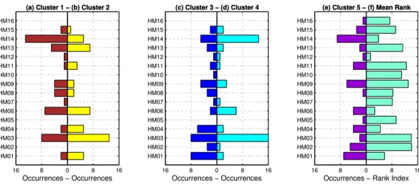
With regard to cluster 4, the regional solution shows a lower diversity of hydrological models. This factor is evi-dent in Fig. 7 which illustrates that for this cluster 70 % of the hydrological members originate from only three hydro-logical models (HM03, HM06, and HM14), which is quite a

different behaviour than for clusters 1, 2 and 3 where the por-tion of the three most selected models reaches 58 %, 56 %, and 44 %, respectively.

Thus it seems that diversity as characteristic of the final se-lection of hydrological members appears to be a factor with a significant impact on the performance of the selection. In other words, the participation of hydrological models in the regional selection stresses the importance of the integration of models with different characteristics. To view this in a de-terministic framework, the index based on the performance rank assigned to each model in each catchment (Sect. 4.2.3) shows that the most selected models (HM01, HM03, HM06, HM09, and HM14) occupy quite different ranks (Fig. 7). For instance, HM03 and HM09 present a high performance while HM01, HM06 and HM14 are of lower performance. This feature exemplifies the notion of the diversity discussed in different stages of the scientific community concerning en-semble methods.

(13)

16 8 0 8 16 HM01 HM02 HM03 HM04 HM05 HM06 HM07 HM08 HM09 HM10 HM11 HM12 HM13 HM14 HM15 HM16

Occurrences − Occurrences

(a) Cluster 1 − (b) Cluster 2

16 8 0 8 16

HM01 HM02 HM03 HM04 HM05 HM06 HM07 HM08 HM09 HM10 HM11 HM12 HM13 HM14 HM15 HM16

(a) Cluster 1 − (b) Cluster 2

16 8 0 8 16

(c) Cluster 3 − (d) Cluster 4

16 8 0 8 16

(c) Cluster 3 − (d) Cluster 4

16 8 0 8 16

Occurrences − Rank Index

(e) Cluster 5 − (f) Mean Rank

16 8 0 8 16

Occurrences − Rank Index

(e) Cluster 5 − (f) Mean Rank

Fig. 7.Hydrological Models participation. Distribution in the five regions (clusters) are presented in(a)–(e). Model performance evaluated as the mean rank index is shown in(f).

Vrugt et al. (2008) proposed positive correlation (lack of di-versity) as an efficient mechanism for removal of members of an ensemble.

Diversity can be defined as the search for models that com-plement their skills, so that each model focuses on different objects. Diversity in the ensemble is thus a vital require-ment for successful modelling. In practice, it appeared to be difficult to define a single measure of diversity and even more difficult to relate that measure to the ensemble performance in a neat and expressive dependency (Kuncheva, 2004). Nev-ertheless, the regional clusters in Fig. 7 make use of most of the 16 available models, whatever their performance rank. For example, the most frequently selected models in cluster 2 are HM03 and HM06 despite the fact that HM02 exhibits the same rank of performance as HM03 and that HM06 presents one of the lowest ranks in the ensemble.

6 Conclusions

A companion paper has already demonstrated the success of the backward greedy member selection technique for sim-plifying a 800-member HEPS combining the 50 perturbed members from the ECMWF MEPS with 16 lumped hydro-logical models (Brochero et al., 2011). The present paper has focused on the generalization quality in time and space of a 50-member HEPS selected from the 800-member en-semble correspondent to the 9-day FTH. When applied to the other 8 time horizons, the 50 selected members also im-proved performance over the initial 800-member HEPS in 82 % of the situations. It was particularly successful when applied to a nearby catchment of the same cluster. Member diversity seems to be the key to this simplified HEPS that makes use of only 6.25 % of the initial structures (50 mem-bers/800 members). Indeed, it has been shown that most 50-member HEPS relied on a broad selection of hydrological

models, which gives further support to the multi-model hy-drological approach.

Comparing scores obtained for the 50 representative hy-drological members to the ones of the initial 800-member ensemble indicated that the proposed selection methodol-ogy, which is based on cross-validation and the combina-tion of scores into a single funccombina-tion, generally leads to good performance in terms of gains of individual scores. However, these gains were not entirely transferable under the scheme of extrapolation evaluated here. This drawback may in part be attributable to the simple selection methodology used here along a linear integration of scores that has no real control over balance, or the need to evaluate more features to en-hance such transferability in the clustering approach.

A more sophisticated approach would optimize all perfor-mance diagnostics simultaneously or find a Pareto set of so-lutions identifying trade-offs among the various performance metrics. Such a framework, but in a context of combina-tion rather than seleccombina-tion of hydrological members, was pro-posed by Vrugt et al. (2006). It consists in the optimization of Bayesian Model Averaging weights and variance using the A Multi-ALgorithm Genetically Adaptive Multiobjective (AMALGAM) method.

Finally, it would be interesting, in the case of a HEPS driven by interchangeable meteorological members, to com-bine the participation of hydrological models found with BGS-CV with the meteorological members chosen by a tech-nique such as that proposed by Molteni et al. (2001) instead of testing them randomly.

Acknowledgements. The authors acknowledge NSERC and the

(14)

Edited by: F. Pappenberger

References

Alpaydin, E.: Introduction to Machine Learning. Adaptive Compu-tation and Machine Learning, 2nd Edn., The MIT Press, Cam-bridge, 2010.

Beven, K. and Binley, A.: The future of distributed models: Model calibration and uncertainty prediction, Hydrol. Process., 6, 279– 298, doi:10.1002/hyp.3360060305, 1992.

Bishop, C. M.: Pattern Recognition and Machine Learning (In-formation Science and Statistics), ISBN0387310738, Springer-Verlag New York, Inc., Secaucus, NJ, USA,2006.

Boucher, M.-A., Perreault, L., and Anctil, F.: Tools for the assessment of hydrological ensemble forecasts ob-tained by neural networks, J. Hydroinform., 11, 297–307, doi:10.2166/hydro.2009.037, 2009.

Bougeault, P., Toth, Z., Bishop, C., Brown, B., Burridge, D., Chen, D. H., Ebert, B., Fuentes, M., Hamill, T. M., Mylne, K., Nico-lau, J., Paccagnella, T., Park, Y.-Y., Parsons, D., Raoult, B., Schuster, D., Dias, P. S., Swinbank, R., Takeuchi, Y., Tennant, W., Wilson, L., and Worley, S.: The THORPEX Interactive Grand Global Ensemble, B. Am. Meteorol. Soc., 91, 1059–1072, doi:10.1175/2010BAMS2853.1, 2010.

Brochero, D., Anctil, F., and Gagn´e, C.: Simplifying a hydrological ensemble prediction system with a backward greedy selection of members – Part 1: Optimization criteria, Hydrol. Earth Syst. Sci., Hydrol. Earth Syst. Sci., 15, 3307–3325, doi:10.5194/hess-15-3307-2011, 2011.

Cloke, H. and Pappenberger, F.: Ensemble flood forecasting: A review, J. Hydrol., 375, 613–626, doi:10.1016/j.jhydrol.2009.06.005, 2009.

Confesor, R. B. and Whittaker, G. W.: Automatic calibration of hydrologic models with multi-objective evolutionary algorithm and pareto optimization, J. Am. Water Resour. Assoc., 43, 981– 989, doi:10.1111/j.1752-1688.2007.00080.x, 2007.

Diamantidis, N., Karlis, D., and Giakoumakis, E.: Unsupervised stratification of cross-validation for accuracy estimation, Artif. Intell., 116, 1–16, doi:10.1016/S0004-3702(99)00094-6, 2000. Ebert, C., B´ardossy, A., and Bliefernicht, J.: Selecting members

of an EPS for flood forecasting systems by using atmospheric circulation patterns, Geophysical Research Abstracts, European Geosciences Union, Vienna, Austria, 9, 2007.

Gneiting, T. and Raftery, A. E.: Strictly proper scoring rules, prediction, and estimation, J. Am. Stat. Assoc., 102, 359–378, doi:10.1198/016214506000001437, 2007.

Gouweleeuw, B. T., Thielen, J., Franchello, G., De Roo, A. P. J., and Buizza, R.: Flood forecasting using medium-range proba-bilistic weather prediction, Hydrol. Earth Syst. Sci., 9, 365–380, doi:10.5194/hess-9-365-2005, 2005.

Gupta, H. V., Sorooshian, S., and Yapo, P. O.: Toward improved calibration of hydrologic models: Multiple and noncommensu-rable measures of information, Water Resour. Res., 34, 751–763, doi:10.1029/97WR03495, 1998.

Gupta, H. V., Bastidas, L. A., Sorooshian, S., Shuttleworth, W. J., and Yang, Z. L.: Parameter estimation of a land surface scheme using multicriteria methods, J. Geophys. Res., 104, 19491– 19503, doi:10.1029/1999JD900154, 1999.

He, Y., Wetterhall, F., Cloke, H. L., Pappenberger, F., Wilson, M., Freer, J., and McGregor, G.: Tracking the uncertainty in flood alerts driven by grand ensemble weather predictions, Meteorol. Appl., 16, 91–101, doi:10.1002/met.132, 2009.

Hudson, M. H. M. and Demuth, H.: Neural Network Toolbox – User’s Guide, The MathWorks, http://www.mathworks.com/ help/pdf doc/allpdf.html, last access: October 2011.

Jaun, S., Ahrens, B., Walser, A., Ewen, T., and Sch¨ar, C.: A probabilistic view on the August 2005 floods in the upper Rhine catchment, Nat. Hazards Earth Syst. Sci., 8, 281–291, doi:10.5194/nhess-8-281-2008, 2008.

Kuncheva, L. I.: Combining Pattern Classifiers: Methods and Al-gorithms, Wiley-Interscience, 2004.

Marsigli, C., Montani, A., Nerozzi, F., Paccagnella, T., Tibaldi, S., Molteni, F., and Buizza, R.: A strategy for high-resolution en-semble prediction, II: Limited-area experiments in four Alpine flood events, Q. J. Roy. Meteorol. Soc., 127, 2095–2115, doi:10.1002/qj.49712757613, 2001.

Molteni, F., Buizza, R., Marsigli, C., Montani, A., Nerozzi, F., and Paccagnella, T.: A strategy for high-resolution ensemble prediction. I: Definition of representative members and global-model experiments, Q. J. Roy. Meteorol. Soc., 127, 2069–2094, doi:10.1002/qj.49712757612, 2001.

Pappenberger, F., Beven, K. J., Hunter, N. M., Bates, P. D., Gouweleeuw, B. T., Thielen, J., and de Roo, A. P. J.: Cas-cading model uncertainty from medium range weather forecasts (10 days) through a rainfall-runoff model to flood inundation pre-dictions within the European Flood Forecasting System (EFFS), Hydrol. Earth Syst. Sci., 9, 381–393, doi:10.5194/hess-9-381-2005, 2005.

Raftery, A. E., Gneiting, T., Balabdaoui, F., and Polakowski, M.: Using Bayesian Model Averaging to calibrate fore-cast ensembles, Mon. Weather Rev., 133, 1155–1174, doi:10.1175/MWR2906.1, 2005.

Roulin, E.: Skill and relative economic value of medium-range hy-drological ensemble predictions, Hydrol. Earth Syst. Sci., 11, 725–737, doi:10.5194/hess-11-725-2007, 2007.

Rousset, F., Habets, F., Martin, E., and Noilhan, J.: Ensemble streamflow forecasts over France, ECMWF Newsletter, 111, 21– 27, 2007.

Todini, E.: Role and treatment of uncertainty in real-time flood forecasting, Hydrol. Process., 18, 2743–2746, doi:10.1002/hyp.5687, 2004.

Vel´azquez, J. A., Anctil, F., Ramos, M. H., and Perrin, C.: Can a multi-model approach improve hydrological ensemble forecast-ing? A study on 29 French catchments using 16 hydrological model structures, Adv. Geosci., 29, 33–42, doi:10.5194/adgeo-29-33-2011, 2011.

Vrugt, J., Diks, C., and Clark, M.: Ensemble Bayesian model aver-aging using Markov Chain Monte Carlo sampling, Environ. Fluid Mech., 8, 579–595, doi:10.1007/s10652-008-9106-3, 2008. Vrugt, J. A. and Robinson, B. A.: Improved evolutionary

optimiza-tion from genetically adaptive multimethod search, P. Natl. Acad. Sci. USA, 104, 708–711, doi:10.1073/pnas.0610471104, 2007. Vrugt, J. A., Clark, M. P., Diks, C. G. H., Duan, Q., and

(15)

Wagener, T., Boyle, D. P., Lees, M. J., Wheater, H. S., Gupta, H. V., and Sorooshian, S.: A framework for development and applica-tion of hydrological models, Hydrol. Earth Syst. Sci., 5, 13–26, doi:10.5194/hess-5-13-2001, 2001.

Wilks, D. S.: Statistical Methods in the Atmospheric Sciences, vol. 91, 2nd Edn., Academic Press, Burlington, MA, London, 2005.

Xuan, Y., Cluckie, I. D., and Wang, Y.: Uncertainty analysis of hydrological ensemble forecasts in a distributed model utilising short-range rainfall prediction, Hydrol. Earth Syst. Sci., 13, 293– 303, doi:10.5194/hess-13-293-2009, 2009.